
8 Systems of Equations and Inequalities
In This Chapter
1.8 Systems of Linear Equations
2.8 Systems of Nonlinear Equations

Student successfully solving a system of linear equations
A Bit of History Many of the mathematical concepts considered in this text are several hundred years old. In this chapter we have a rare opportunity to examine, albeit briefly, a topic that has its origins in the twentieth century. Linear programming, like many other branches of mathematics, originated in an attempt to solve practical problems. But unlike the mathematics of earlier centuries, which was often rooted in the sciences of physics and astronomy, linear programming developed from an effort to solve problems in business, manufacturing, shipping, economics, and military planning. In these problems it was usually necessary to find the optimal values (that is, maximum and minimum values) of a linear function when certain restrictions were placed on the variables. There was no general mathematical procedure for solving this kind of problem until George B. Dantzig (1914-2005) published his simplex method in 1947. Dantzig and his colleagues in the U.S. Air Force developed this method for finding optimal values of a linear function by investigating certain problems in transportation and military logistical planning. The word “programming,” it should be pointed out, does not refer to computer programming but rather to a program of action.
Although we will not study the simplex method itself, we will see in Section 8.5 that linear-programming problems involving two variables can be solved in a geometric manner.
8.1 Systems of Linear Equations
![]() Introduction Recall from Section 3.3 that a linear equation in two variables x and y is any equation that can be put in the form ax + by = c, where a and b are real numbers not both zero. In general, a linear equation in n variables x1, x2,…, xn is an equation of the form
Introduction Recall from Section 3.3 that a linear equation in two variables x and y is any equation that can be put in the form ax + by = c, where a and b are real numbers not both zero. In general, a linear equation in n variables x1, x2,…, xn is an equation of the form
![]()
where the real numbers a1, a2,…, an are not all zero. The number b is called the constant term of the equation. The equation in (1) is also called a first-degree equation in that the exponent of each of the n variables is 1. In this and the next section we examine solution methods for systems of equations.
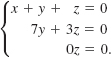
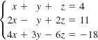
![]() Terminology A system of equations consists of two or more equations with each equation containing at least one variable. If each equation in a system is linear, we say that it is a system of linear equations or simply a linear system. Whenever possible, we will use the familiar symbols x, y, and z to represent variables in a system. For example,
Terminology A system of equations consists of two or more equations with each equation containing at least one variable. If each equation in a system is linear, we say that it is a system of linear equations or simply a linear system. Whenever possible, we will use the familiar symbols x, y, and z to represent variables in a system. For example,
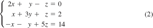
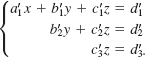
is a linear system of three equations in three variables. The brace in (2) is just a way of reminding us that we are trying to solve a system of equations and that the equations must be dealt with simultaneously. A solution of a system of n equations in n variables consists of values of the variables that satisfy each equation in the system. A solution of such a system is also written as an ordered n-tuple. For example, as we see x = 2, y = – 1, and z = 3 satisfy each equation in the linear system (2):
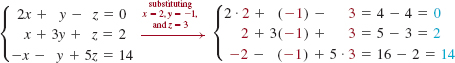
and so these values constitute a solution. Alternatively, this solution can be written as the ordered triple (2, –1, 3). To solve a system of equations we find all solutions of the system. Often to solve a system of equations we perform operations on the system to transform it into an equivalent set of equations. Two systems of equations are said to be equivalent if they have precisely the same solution sets.
![]() Linear Systems in Two Variables The simplest linear system consists of two equations in two variables:
Linear Systems in Two Variables The simplest linear system consists of two equations in two variables:
![]()
Because the graph of a linear equation ax + by = c is a straight line, the system determines two straight lines in the xy-plane.
![]() Consistent and Inconsistent Systems As shown in FIGURE 8.1.1 there are three possible cases for the graphs of the equations in system (3):
Consistent and Inconsistent Systems As shown in FIGURE 8.1.1 there are three possible cases for the graphs of the equations in system (3):
 The lines intersect in a single point.
 ![]()
The equations describe coincident lines. ![]()
The two lines are parallel. ![]()
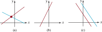
FIGURE 8.1.1Two lines in the plane
In these three cases we say, respectively;
The system is consistent and the equations are independent. The system has exactly one solution, that is, the ordered pair of real numbers corresponding to the point of intersection of the lines.
The system is consistent, but the equations are dependent. The system has infinitely many solutions, that is, all the ordered pairs of real numbers corresponding to the points on the one line.
The system is inconsistent. The lines are parallel and so there are no solutions.
For example, the equations in the linear system
![]()
are parallel lines as in Figure 8.1.1(c). Hence the system is inconsistent.
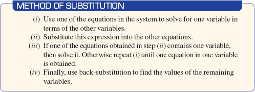
To solve a system of linear equations, we can use either the method of substitution or the method of elimination.
![]() Method of Substitution The first solution technique considered is called the method of substitution.
Method of Substitution The first solution technique considered is called the method of substitution.
EXAMPLE 1 Method of Substitution
Solve the system
![]()
Solution Solving the second equation for y yields
![]()
We substitute this expression into the first equation and solve for x:
![]()
Back-substitution ![]()
We then substitute this value back into the first equation:
![]()
Solution written as an ordered pair. ![]()
Thus the only solution of the system is (1, - 2). The system is consistent and the equations are independent.
![]() Linear Systems in Three Variables In calculus it is shown that the graph of a linear equation in three variables,
Linear Systems in Three Variables In calculus it is shown that the graph of a linear equation in three variables,
![]()
where a, b, and c are not all zero, determines a plane in three-dimensional space. As we have seen in (2), a solution of a system of three equations in three unknowns
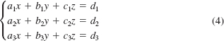
is an ordered triple of the form (x, y, z); an ordered triple of numbers represents a point in three-dimensional space. The intersection of the three planes described by the system (4) may be
a single point,
infinitely many points, or
no points.
As before, to each of these cases we apply the terms consistent and independent, consistent and dependent, and inconsistent, respectively. Each is illustrated in FIGURE 8.1.2.
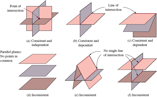
FIGURE 8.1.2 Three planes in three dimensions
![]() Method of Elimination The next method that we illustrate uses elimination operations. When applied to a system of equations, these operations yield an equivalent system of equations.
Method of Elimination The next method that we illustrate uses elimination operations. When applied to a system of equations, these operations yield an equivalent system of equations.
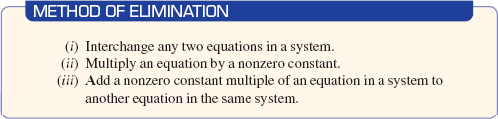
We often add a nonzero constant multiple of one equation to other equations in a system with the intention of eliminating a variable from those equations.
For convenience, we represent these operations by the following symbols, where the letter E stands for the word equation:
Ei ↔ Ej: Interchange the i th equation with the j th equation.
kEi: Multiply the i th equation by a constant k.
kEi + Ej: Multiply the ith equation by k and add to the j th equation.
Reading a linear system from the top, E1 represents the first equation, E2 represents the second equation, and so on.
Using the method of elimination it is possible to reduce the system (4) of three linear equations in three variables to an equivalent system in triangular form,
A solution of the system (if one exists) can be readily obtained by back-substitution. The next example illustrates the procedure.
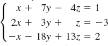
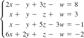
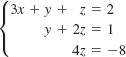
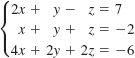
EXAMPLE 2 Elimination and Back Substitution
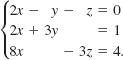
Solve the system
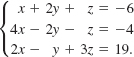
Solution We begin by eliminating x from the second and third equations:
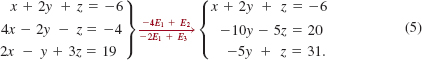
We then eliminate y from the third equation and obtain an equivalent system in triangular form:
We arrive at another triangular form that is equivalent to the original system by multiplying the third equation by ![]() :
:
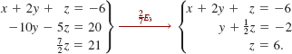
From this last system it is evident that z = 6. Using this value and substituting back into the second equation gives
![]()
Finally, by substituting y = – 5 and z = 6 back into the first equation, we obtain
![]()
The answer indicates that the three planes intersect at a point as in FIGURE 8.1.2 (a). ![]()
Therefore the solution of the system is (–2, –5, 6).
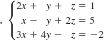
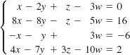
EXAMPLE 3 Elimination and Back Substitution
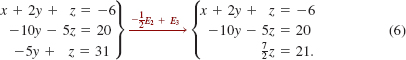
Solve the system
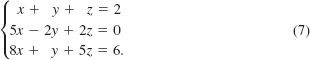
Solution Using the first equation to eliminate the variable x from the second and third equations, we get the equivalent system
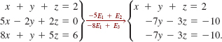
This system, in turn, is equivalent to the system in triangular form:
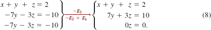
In this system we cannot determine unique values for x, y, and z. At best we can solve for two variables in terms of the remaining variable. For example, from the second equation in (8), we obtain y in terms of z:
![]()
Substituting this equation for y in the first equation for x gives
![]()
The answer indicates that the two planes intersect in a line as in FIGURE 8.1.2 (b).![]()
Thus in the solutions for y and x, we can choose z arbitrarily. If we denote z by the symbol α, where α represents a real number, then the solutions of the system are all ordered triples of the form ![]() .We emphasize that for any real number α, we obtain a solution of (7). For example, by choosing α to be, say, 0, 1, and 2, we obtain the solutions
.We emphasize that for any real number α, we obtain a solution of (7). For example, by choosing α to be, say, 0, 1, and 2, we obtain the solutions ![]() , respectively. In other words, the system is consistent and has infinitely many solutions.
, respectively. In other words, the system is consistent and has infinitely many solutions.
In Example 3 there is nothing special about solving (8) for x and y in terms of z. For instance, by solving (8) for x and z in terms of y, we obtain the solution ![]() , where β is any real number. Note that by setting β equal to
, where β is any real number. Note that by setting β equal to ![]() , 1, and
, 1, and ![]() , we get the same solutions in Example 3 corresponding, in turn, to α = 0, α = 1, and α = 2.
, we get the same solutions in Example 3 corresponding, in turn, to α = 0, α = 1, and α = 2.
EXAMPLE 4 No Solution
Solve the system
Solution The elimination method,
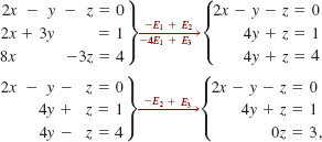
shows that the last equation 0z = 3 is never satisfied for any number z since 0 ≠ 3. Thus, the system is inconsistent and so has no solutions.
![]() Homogeneous Systems A linear system in which all the constant terms are zero, such as,
Homogeneous Systems A linear system in which all the constant terms are zero, such as,
![]()
or
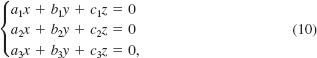
is said to be homogeneous. Note that systems (9) and (10) have the solutions (0, 0) and (0, 0, 0), respectively. A solution of a system of equations in which each of its variables is zero is called the zero solution or the trivial solution. Because a homogeneous linear system always possesses at least the zero solution, such a system is always consistent. In addition to the zero solution, however, there may exist infinitely many nonzero solutions. These solutions can be found by proceeding exactly as in Example 3.
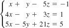
EXAMPLE 5 A Homogeneous System
The same steps used to solve the system in Example 3 can be used to solve the related homogeneous system
In this case the elimination steps yield
Choosing z = α, where α is a real number, we find from the second equation of the last system that ![]() . Then using the first equation, we obtain
. Then using the first equation, we obtain ![]() . Thus, the solutions of the system consist of all ordered triples of the form
. Thus, the solutions of the system consist of all ordered triples of the form ![]() . Note that for α = 0, we obtain the trivial solution (0, 0, 0) but for, say, α = –7, we obtain the nontrivial solution (4, 3, –7).
. Note that for α = 0, we obtain the trivial solution (0, 0, 0) but for, say, α = –7, we obtain the nontrivial solution (4, 3, –7).
The discussion in this section is also applicable to systems of n linear equations in n variables for n > 3. See Problems 25 and 26 in Exercises 8.1.
8.1 Exercises Answers to selected odd-numbered problems begin on page ANS-19.
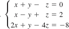
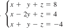
In Problems 1-26, solve the given linear system. State whether the system is consistent, with independent or dependent equations, or whether it is inconsistent.
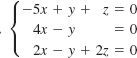
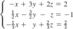
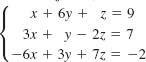
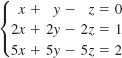
1. ![]()
2. ![]()
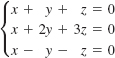
3. ![]()
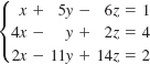
4. ![]()
5. ![]()
6. ![]()
7. ![]()
8. ![]()
9. ![]()
10. ![]()
11. 
12. 
13. 
14. 
15. 
16. 
17. 
18. 
19. 
20. 
21. 
22. 
23. 
24. 
25. 
26. 
In Problems 27-30, solve the given system.
27. 
28. 
29. ![]()
30. ![]()
Miscellaneous Applications
31. Speed An airplane flies 3300 mi from Hawaii to California in 5.5 h with a tailwind. From California to Hawaii, flying against a wind of the same velocity, the trip takes 6 h. Determine the speed of the plane and the speed of the wind.
32. How Many Coins? A person has 20 coins, consisting of dimes and quarters, which total $4.25. Determine how many of each coin the person has.
33. Number of Gallons A 100-gal tank is full of water in which 50 lb of salt is dissolved. A second tank contains 200 gal of water with 75 lb of salt. How much should be removed from both tanks and mixed together in order to make a solution of 90 gal with ![]() lb of salt per gallon?
lb of salt per gallon?
34. Playing with Numbers The sum of three numbers is 20. The difference of the first two numbers is 5, and the third number is 4 times the sum of the first two. Find the numbers.
35. How Long? Three pumps P1, P2, and P3 working together can fill a tank in 2 h. Pumps P1 and P2 can fill the same tank in 3 h, whereas pumps P2 and P3 can fill it in 4 h. Determine how long it would take each pump working alone to fill the tank.
36. Parabola Through Three Points The parabola y = ax2 + bx + c passes through the points (1, 10), (–1, 12), and (2, 18). Find a, b, and c.
37. Area Find the area of the right triangle shown in FIGURE 8.1.3.
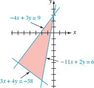
FIGURE 8.1.3 Triangle in Problem 37
38. Current According to Kirchhoff's law of voltages, the currents i1, i2, and i3 in the parallel circuit shown in FIGURE 8.1.4 satisfy the equations
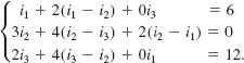
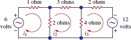
FIGURE 8.1.4 Circuit in Problem 38
Solve for i1, i2, and i3.
39. The A, B, C's When Beth graduated from college, she had completed 40 courses, in which she received grades of A, B, and C. Her final GPA (grade point average) was 3.125. Her GPA in only those courses in which she received grades of A and B was 3.8. Assume that A, B, and C grades are worth 4 points, 3 points, and 2 points, respectively. Determine the number of A's, B's, and C's that Beth received.
40. (a) To find ten distinct lines of the form y = mix + bi, mi ≠ 0, i = 1, 2,…, 10, so that the graph of each line passes through the point (1, 1), explain why we must find the values of twenty variables that satisfy:
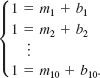
(b) From part (a) find a relationship between mi and bi.
(c) Use part (b) to find ten different lines passing through the point (1, 1).
For Discussion
41. Determine conditions on a1, a2,b1, and b2 so that the linear system (9) has only the trivial solution.
42. Determine a value of k such that the linear system
![]()
is (a) inconsistent and (b) dependent.
43. Devise a system of two linear equations whose solution is (2,-5).
44. Devise a system of three linear equations whose solution is (1, 1, 1).
8.2 Systems of Nonlinear Equations
![]() Introduction As FIGURE 8.2.1 illustrates, the graphs of the parabolas y = x2 – 4x and y = –x2 + 8 intersect at two points. Thus the coordinates of the points of intersection must satisfy both equations,
Introduction As FIGURE 8.2.1 illustrates, the graphs of the parabolas y = x2 – 4x and y = –x2 + 8 intersect at two points. Thus the coordinates of the points of intersection must satisfy both equations,
![]()
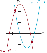
FIGURE 8.2.1 Intersection of two parabolas
Recall from Sections 3.3 and 8.1 that any equation that can be put in the form ax + by + c = 0 is called a linear equation in two variables. A nonlinear equation is simply one that is not linear. For example, in system (1) both equations y =x2 – 4x and y = –x2 + 8 are nonlinear. A system of equations in which at least one of the equations is nonlinear will be referred to as a system of nonlinear equations or simply a nonlinear system.
In the examples that follow, will use the methods of substitution and elimination introduced in Section 8.1 to solve nonlinear systems.
EXAMPLE 1 Solution of (l)
Find the solutions of the system (1).
Solution Since the first equation already expresses y in terms of x, we substitute this expression for y into the second equation to get a single equation in one variable:
![]()
Simplifying the last equation we get a quadratic equation x2 – 2x – 4 = 0that we solve using the quadratic formula: x = 1 – ![]() and x = 1 +
and x = 1 + ![]() . We then substitute each of these numbers back into the first equation in (1) to solve for the corresponding values of y. This gives
. We then substitute each of these numbers back into the first equation in (1) to solve for the corresponding values of y. This gives
![]()
Thus, ![]() are solutions of the system.
are solutions of the system.
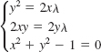
EXAMPLE 2 Solving a Nonlinear System
Find the solutions of the system
![]()
Solution From the second equation, we have x = 10y, and therefore x2 = 102y. Substituting this last result into the first equation gives
![]()
Since x2 + 1 > 0 for all real numbers x, it follows that x2 = 3 or x = ± ![]() . But x = 10y > 0 for all y; therefore, we must take x =
. But x = 10y > 0 for all y; therefore, we must take x = ![]() . Solving
. Solving ![]() = 10 y for y gives
= 10 y for y gives
![]()
Hence, ![]() is the only solution of the system.
is the only solution of the system.
![]() Solution written by specifying values of the variables.
Solution written by specifying values of the variables.
EXAMPLE 3 Dimensions of a Rectangle
Consider a rectangle in the first quadrant bounded by the x– and y–axes and the graph of y = 20 – x2. See FIGURE 8.2.2. Find the dimensions of such a rectangle if its area is 16 square units.
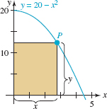
FIGURE 8.2.2 Rectangle in Example 3
Solution Let (x, y) be the coordinates of the point P on the graph of y = 20 – x2 shown in the figure. Then the
![]()
Thus we obtain the system of equations
![]()
The first equation of the system yields y =16/x After substituting this expression for y in the second equation, we get
![]()
or
![]()
Now from the Rational Zeros Theorem in Section 5.4 the only possible rational roots of the last equation are ±1, ±2, ±4, ±8, and ±16. Testing these numbers by synthetic division eventually shows that

and so 4 is a solution. But the division above gives the factorization
![]()
Applying the quadratic formula to x2 + 4x – 4 = 0 reveals two more real roots:
![]()
The positive number –2 + 2 ![]() is another solution. Since dimensions are positive, we reject the negative number –2 – 2
is another solution. Since dimensions are positive, we reject the negative number –2 – 2 ![]() . In other words, there are two rectangles with area 16 square units.
. In other words, there are two rectangles with area 16 square units.
To find y, we use y = 16/x. If x = 4, then y = 4, and if ![]() , then
, then ![]() . Thus the dimensions of the two rectangles are
. Thus the dimensions of the two rectangles are
![]()
Note: In Example 3 observe that the equation 16 = 20x – x x3 was obtained by multiplying the equation preceding it by x. Remember, when equations are multiplied by a variable, there is the possibility of introducing an extraneous solution. To make sure that this is not the case, you should check each solution.
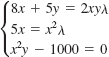
EXAMPLE 4 Solving a Nonlinear System
Find the solutions of the system
![]()
Solution In preparation for eliminating an x2–term, we begin by multiplying the first equation by 2. The system
![]()
is equivalent to the given system. Now, by adding the first equation of this last system to the second, we obtain yet another system equivalent to the original system. In this case, we have eliminated x2 from the second equation
![]()
From the last equation, we see that ![]() . Substituting these two values of y into x2 + y2 = 4 then gives
. Substituting these two values of y into x2 + y2 = 4 then gives
![]()
so that ![]() , and
, and ![]() are all solutions. The graphs of the given equations and the four points corresponding to the ordered pairs are indicated by the red dots in FIGURE 8.2.3.
are all solutions. The graphs of the given equations and the four points corresponding to the ordered pairs are indicated by the red dots in FIGURE 8.2.3.
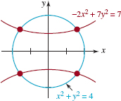
FIGURE 8.2.3 Intersection of a circle and a hyperbola in Example 4
In Example 4 we note that the system can also be solved by the substitution method by substituting, say, y2 = 4 – x2 into the second equation.
In the next example, we use the third elimination operation to simplify the system before applying the substitution method.
EXAMPLE 5 Solving a Nonlinear System
Find the solutions of the system
![]()
Solution By multiplying the first equation by – 1 and adding the result to the second, we eliminate x2 and y2 from that equation:
![]()
The second equation of the latter system implies that y = x. Substituting this expression into the first equation then yields
![]()
It follows that x = 0, x = 1 and, correspondingly, y = 0, y = 1. Thus the solutions of the system are (0, 0) and (1, 1).
By completing the square in x and y, we can write the system in Example 5 as
![]()
From this system we see that both equations describe circles of radius r = 1. The circles and their points of intersection are illustrated in FIGURE 8.2.4.
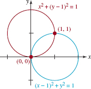
FIGURE 8.2.4 Intersecting circles in Example 5
8.2 Exercises Answers to selected odd-numbered problems begin on page ANS-20.
In Problems 1–6, determine graphically whether the given nonlinear system has any solutions.
1. ![]()
2. ![]()
3. ![]()
4. ![]()
5. ![]()
6. ![]()
In Problems 7–38, solve the given nonlinear system.
7. ![]()
8. ![]()
9. ![]()
10. ![]()
11. ![]()
12. ![]()
13. 
14. ![]()
15. ![]()
16. ![]()
17. ![]()
18. ![]()
19. ![]()
20. ![]()
21. ![]()
22. ![]()
23. ![]()
24. ![]()
25. ![]()
26. ![]()
27. ![]()
28. ![]()
29. ![]()
30. ![]()
31. ![]()
32. ![]()
33. ![]()
34. ![]()
35. 
36. 
37. 
38. 
Miscellaneous Applications
39. Dimensions of a Corral The perimeter of a rectangular corral is 260 ft and its area is 4000 ft2. What are its dimensions?
40. Inscribed Rectangle Find the dimensions of the rectangle(s) with area 10 cm2inscribed in the triangle consisting of the blue line and the two coordinate axes shown in FIGURE 8.2.5.
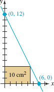
FIGURE 8.2.5 Rectangle in Problem 40
41. Sum of Areas The sum of the radii of two circles is 8 cm. Find the radii if the sum of the areas of the circles is 32π cm2.
42. Intersecting Circles Find the two points of intersection of the circles shown in FIGURE 8.2.6 if the radius of each circle is ![]()
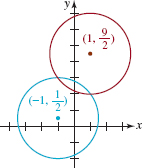
FIGURE 8.2.6 Circles in Problem 42
43. Golden Ratio The golden ratio for the rectangle shown in FIGURE 8.2.7 is defined by
![]()
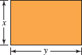
FIGURE 8.2.7 Rectangle in Problem 43
This ratio is often used in architecture and in paintings. Find the dimensions of a rectangular sheet of paper containing 100 in2 that satisfy the golden ratio.
44. Length The hypotenuse of a right triangle is 20 cm. Find the lengths of the remaining two sides if the shorter side is one–half the length of the longer side.
45. Topless Box A box is to be made with a square base and no top. See FIGURE 8.2.8. The volume of the box is to be 32 ft3, and the combined areas of the sides and bottom are to be 68 ft2. Find the dimensions of the box.
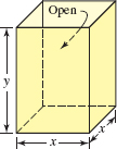
FIGURE 8.2.8 Open box in Problem 45
46. Dimensions of a Cylinder The volume of a right circular cylinder is 63π in 3, and its height h is 1 in. greater than twice its radius r. Find the dimensions of the cylinder.
For Discussion
47. A tangent to an ellipse is defined exactly as it was for the circle, namely, a straight line that touches the ellipse at only one point (x1 y1). See Problem 42 in Exercises 3.3. It can be shown (see Problem 48) that an equation of the tangent line at a given point (x1, y1) on an ellipse ![]()
![]()
(a) Find the equation of the tangent line to the ellipse ![]() at the point (5, –2).
at the point (5, –2).
(b) Write your answer in the form of y = mx + b.
(c) Sketch the ellipse and the tangent line.
48. In this problem, you are guided through the steps to derive equation (3).
(a) An alternative form of the equation ![]()
![]()
Since the point (x1, y1) is on the ellipse, its coordinates must satisfy the foregoing equation:
![]()
Show that
![]()
(b) Using the point–slope form of a line, the tangent line at (x1, y1) is y – y1 =m(x – x1).Use substitution in the system
![]()
to show that
![]()
The last equation is a quadratic equation in x. Explain why x1 is a repeated root or a root of multiplicity 2.
(c) By factoring, (4) becomes
![]()
and so we must have
![]()
Use the last equation to find the slope m of the tangent line at (x1, y1). Finish the problem by finding the equation of the tangent as given in (3).
8.3 Partial Fractions
![]() Introduction When two rational functions, say,
Introduction When two rational functions, say, ![]() are added, the terms are combined by means of a common denominator:
are added, the terms are combined by means of a common denominator:
![]()
Adding numerators on the right–hand side of (1) yields the single rational expression
![]()
An important procedure in the study of integral calculus requires that we be able to reverse the process; in other words, starting with a rational expression such as (2) break it down, or decompose it, into simpler component fractions 2/(x + 5) and 1/(x + 1) called partial fractions.
![]() Terminology The algebraic process for breaking down a rational expression such as (2) into partial fractions is known as partial fraction decomposition. For convenience we will assume that the rational function P(x)/Q(x), Q(x) ≠ 0, is a properfraction or proper rational expression; that is, the degree of P(x) is less than the degree of Q(x). We will also assume once again that the polynomials P(x) and Q(x) have no common factors.
Terminology The algebraic process for breaking down a rational expression such as (2) into partial fractions is known as partial fraction decomposition. For convenience we will assume that the rational function P(x)/Q(x), Q(x) ≠ 0, is a properfraction or proper rational expression; that is, the degree of P(x) is less than the degree of Q(x). We will also assume once again that the polynomials P(x) and Q(x) have no common factors.
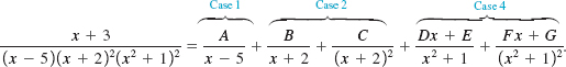
In the discussion that follows we consider four cases of partial fraction decomposition of P(x)/Q(x). The cases depend on the factors in the denominator Q(x). When the polynomial Q(x) is factored as a product of (ax + b)n and (ax2 + bx + c)m, n = 1, 2,…, m = 1, 2,…, where the coefficients a, b, c are real numbers and the quadratic polynomial ax2 + bx + c is irreducible over the real numbers (that is, does not factor using real numbers), the rational expression P(x)/Q(x) can be decomposed into a sum of partial fractions of the form
![]()
CASE 1: Q(x) Contains Only Nonrepeated Linear Factors
We state the following fact from algebra without proof. If the denominator can be factored completely into linear factors,
![]()
where all the aix + bi, i = 1, 2,…, n are distinct (that is, no two factors are the same), then unique real constants C1, C2,…, Cn can be found such that
![]()
In practice we will use the letters A, B, C,…in place of the subscripted coefficients C1, C2, C3,…The next example illustrates this first case.
EXAMPLE 1 Distinct Linear Factors
To decompose ![]() into individual partial fractions we make the assumption, based on the form given in (3), that the rational function can be written as
into individual partial fractions we make the assumption, based on the form given in (3), that the rational function can be written as
![]()
We now clear (4) of fractions; this can be done by either combining the terms on the right– hand side of the equality over a least common denominator and equating numerators or by simply multiplying both sides of the equality by the denominator (x – 1)(x + 3) on the left–hand side. Either way, we arrive at
![]()
Multiplying out the right–hand side of (5) and grouping by powers of x gives
![]()
Each of the equations (5) and (6) is an identity, which means that the equality is true for all real values of x. As a consequence, the coefficients of x on the left–hand side of (6) must be the same as the coefficients of the corresponding powers of x on the right–hand side, that is,
![]()
The result is a system of two linear equations in two variables A and B:
![]()
By adding the two equations we get 3 = 4A and so we find that ![]() Substituting this value into either equation in (7) then yields
Substituting this value into either equation in (7) then yields ![]() . Hence the desired decomposition is
. Hence the desired decomposition is
![]()
You are encouraged to verify the foregoing result by combining the terms on the right–hand side of the last equation by means of a common denominator.
![]() A Shortcut Worth Knowing If the denominator contains, say, three linear factors such as in
A Shortcut Worth Knowing If the denominator contains, say, three linear factors such as in ![]() , then the partial fraction decomposition looks like this
, then the partial fraction decomposition looks like this
![]()
By following the same steps as in Example 1, we would find that the analog of (7) is now three equations in the three unknowns A,B, and C. The point is this: The more linear factors in the denominator the larger the system of equations we must solve. There is a procedure worth learning that can cut down on some of the algebra. To illustrate, let's return to the identity (5). Since the equality is true for every value of x, it holds for x = 1 and x = –3, the zeros of the denominator. Setting x = 1 in (5) gives 3 = 4A, from which it follows immediately that ![]() . Similarly, by setting x = –3 in (5), we obtain –5 = (–4)B or
. Similarly, by setting x = –3 in (5), we obtain –5 = (–4)B or ![]() .
.
CASE 2:Q(x) Contains Repeated Linear Factors
If the denominator Q(x) contains a repeated linear factor (ax + b)n,n > 1, then unique real constants C1, C2,…, Cn can be found such that the partial fraction decomposition of P(x)/Q(x) contains the terms
![]()
EXAMPLE 2 Repeated Linear Factors
To decompose ![]() into partial fractions we first observe that the denominator consists of the repeated linear factor x and the nonrepeated linear factor 2x – 1. Based on the forms in (3) and (8) we assume that
into partial fractions we first observe that the denominator consists of the repeated linear factor x and the nonrepeated linear factor 2x – 1. Based on the forms in (3) and (8) we assume that
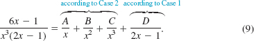
Multiplying (9) by x3(2x – 1) clears it of fractions and yields
![]()
or
![]()
Now the zeros of the denominator in the original expression are x = 0 and ![]() If we then set x = 0 and
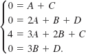
If we then set x = 0 and ![]() in (10), we find, in turn, that C = 1 and D = 16. Because the denominator of the original expression has only two distinct zeros, we can find A and B by equating the corresponding coefficients of x3 and x2 in (11):
in (10), we find, in turn, that C = 1 and D = 16. Because the denominator of the original expression has only two distinct zeros, we can find A and B by equating the corresponding coefficients of x3 and x2 in (11):
The coefficients of x3 and x2 on the left-hand side of (11) are both 0.![]()
![]()
Using the known value of D, the first equation yields A = –D/2 = –8. The second then gives B = A/2 = –4. The partial fraction decomposition is
![]()
CASE 3: Q(x) Contains Nonrepeated Irreducible Quadratic Factors
If the denominator Q(x) contains nonrepeated irreducible quadratic factors ai x2 + bi x + ci, then unique real constants A1, A2,…, An, B1, B2,…, Bn can be found such that the partial fraction decomposition of P(x)/Q(x) contains the terms
![]()
EXAMPLE 3 Irreducible Quadratic Factors
![]() Use the quadratic formula. For either factor you will find that b2 – 4ac < 0.
Use the quadratic formula. For either factor you will find that b2 – 4ac < 0.
To decompose ![]() into partial fractions we first observe that the quadratic polynomials x2 + 1 and x2 + 2x + 3 are irreducible over the real numbers. Hence by (12) we assume that
into partial fractions we first observe that the quadratic polynomials x2 + 1 and x2 + 2x + 3 are irreducible over the real numbers. Hence by (12) we assume that
![]()
After clearing fractions in the preceding line, we find
![]()
Because the denominator of the original fraction has no real zeros, we have no recourse except to form a system of equations by comparing coefficients of all powers of x:
Using C = –A and D = –3B from the first and fourth equations we can eliminate C and D in the second and third equations:
![]()
Solving this simpler system of equations yields A = 1 and B = 1. Hence, C = –1 and D = –3. The partial fraction decomposition is
![]()
CASE 4: Q(x) Contains Repeated Irreducible Quadratic Factors
If the denominator Q(x) contains a repeated irreducible quadratic factor (ax2 + bx + c)n, n > 1, then unique real constants A1, A2,…, An, B1, B2,…, Bn can be found such that the partial fraction decomposition of P(x)/Q(x) contains the terms
![]()
EXAMPLE 4 Repeated Quadratic Factor
Decompose ![]() into partial fractions.
into partial fractions.
Solution The denominator contains only the repeated irreducible quadratic factor x2 + 4. As indicated in (13) we assume a decomposition of the form
![]()
Clearing fractions by multiplying both sides of the preceding equality by (x2 + 4)2 gives
![]()
As in Example 3, the denominator of the original has no real zeros and so we must solve a system of four equations for A, B, C, and D. To that end we rewrite (14) as
![]()
and compare coefficients of like powers (match the colors) to obtain

From this system we find that A = 0, B = 1, C = 0, and D = –4. The required partial fraction decomposition is then
![]()
EXAMPLE 5 Combination of Cases
Determine the form of the decomposition of ![]()
Solution The denominator contains a single linear factor x – 5, a repeated linear factor x + 2, and a repeated irreducible quadratic factor x2 + 1. By Cases 1, 2, and 4 the assumed form of the partial fraction decomposition is
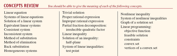
NOTES FROM THE CLASSROOM

We assumed throughout the foregoing discussion that the degree of the numerator P(x) was less than the degree of the denominator Q(x). If, however, the degree of P(x) is greater than or equal to the degree of Q(x), then P(x)/Q(x) is an improper fraction. We can still do partial fraction decomposition but the process starts with long division until a polynomial quotient and a proper fraction is attained. For example, long division gives
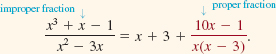
Then by using Case 1 we finish the problem with the decomposition of the proper fraction term in the last equality:
![]()
8.3 Exercises Answers to selected odd-numbered problems begin on page ANS-20.
In Problems 1–24, find the partial fraction decomposition of the given rational expression.
1. ![]()
2. ![]()
3. ![]()
4. ![]()
5. ![]()
6. ![]()
7. ![]()
8. ![]()
9. ![]()
10. ![]()
11. ![]()
12. ![]()
13. ![]()
14. ![]()
15. ![]()
16. ![]()
17. ![]()
18. ![]()
19. ![]()
20. ![]()
21. ![]()
22. ![]()
23. ![]()
24. ![]()
In Problems 25–30, first use long division followed by partial fraction decomposition.
25. ![]()
26. ![]()
27. ![]()
28. ![]()
29. ![]()
30. ![]()
8.4 Systems of Inequalities
![]() Introduction In Chapter 002 we solved linear and nonlinear inequalities involving a single variable x and then graphed the solution set of the inequality on the number line. In this section our focus will be on inequalities involving two variables x and y. For example,
Introduction In Chapter 002 we solved linear and nonlinear inequalities involving a single variable x and then graphed the solution set of the inequality on the number line. In this section our focus will be on inequalities involving two variables x and y. For example,
![]()
are inequalities in two variables. A solution of an inequality in two variables is any ordered pair of real numbers (x0, y0) that satisfies the inequality—that is, results in a true statement—when x0 and y0 are substituted for x and y, respectively. A graph of the solution set of an inequality in two variables is made up of all points in the plane whose coordinates satisfy the inequality.
Many results obtained in higher-level mathematics courses are valid only in a specialized region either in the xy-plane or in three-dimensional space, and these regions are often defined by means of systems of inequalities in two or three variables. In this section we consider only systems of inequalities involving two variables x and y.
We begin with linear inequalities in two variables.
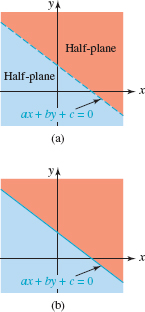
FIGURE 8.4.1 A single line determines two half-planes
![]() Half-Planes A linear inequality in two variables x and y is any inequality that has one of the forms
Half-Planes A linear inequality in two variables x and y is any inequality that has one of the forms
![]()
![]()
Since the inequalities in (1) and (2) have infinitely many solutions, the notation
![]()
and so on, is used to denote a set of solutions. Geometrically, each of these sets describes a half-plane. As shown in FIGURE 8.4.1, the graph of the linear equation ax + by + c = 0 divides the xy-plane into two regions, or half-planes. One of these half- planes is the graph of the set of solutions of the linear inequality. If the inequality is strict, as in (1), then we draw the graph of ax + by + c = 0 as a dashed line, because the points on the line are not in the set of solutions of the inequality. See Figure 8.4.1(a). On the other hand, if the inequality is nonstrict, as in (2), the set of solutions includes the points satisfying ax + by + c = 0, and so we draw the graph of the equation as a solid line. See Figure 8.4.1(b).
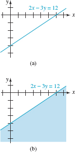
FIGURE 8.4.2 Half-plane in Example 1
EXAMPLE 1 Graph of a Linear Inequality
Graph the linear inequality 2x – 3y ≥ 12.
Solution First, we graph the line 2x – 3y = 12, as shown in Figure 8.4.2(a). Solving the given inequality for y gives
![]()
Since the y-coordinate of any point (x, y) on the graph of 2x – 3y ≥ 12 must satisfy (3), we conclude that the point (x, y) must lie on or below the graph of the line. This solution set is the region that is shaded blue in Figure 8.4.2(b).
Alternatively, we know that the set
![]()
describes a half-plane. Thus we can determine whether the graph of the inequality includes the region above or below the line 2x – 3y = 12 by determining whether a test point not on the line, such as (0, 0), satisfies the original inequality. Substituting x = 0, y = 0 into 2x – 3y ≥ 12 gives 0 ≥ 12. This false statement implies that the graph of the inequality is the region on the other side of the line 2x – 3y = 12, that is, the side that does not contain the origin. Note that the blue half-plane in Figure 8.4.2(b) does not contain the point (0, 0).
In general, given a linear inequality of the forms in (1) or (2), we can graph the solutions by proceeding in the following manner.
![]() Graph the line ax + by + c = 0.
Graph the line ax + by + c = 0.
![]() Select a test point not on this line.
Select a test point not on this line.
![]() Shade the half-plane containing the test point if its coordinates satisfy the original inequality. If they do not satisfy the inequality, shade the other half-plane.
Shade the half-plane containing the test point if its coordinates satisfy the original inequality. If they do not satisfy the inequality, shade the other half-plane.
EXAMPLE 2 Graph of a Linear Inequality
Graph the linear inequality 3x + y – 2 < 0.
Solution In FIGURE 8.4.3 we draw the graph of 3x + y = 2 as a dashed line, since it will not be part of the solution set of the inequality. Then we select (0, 0) as a test point that is not on the line. Because substituting x = 0, y = 0 into 3x + y – 2 < 0 gives the true statement –2 < 0 we shade that region of the plane containing the origin.
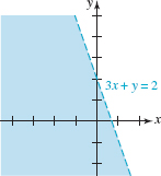
FIGURE 8.4.3 Half-plane in Example 2
![]() Systems of Inequalities We say (x0, y0) is a solution of a system of inequalities when it is a member of the set of solutions common to all inequalities. In other words, the solution set of a system of inequalities is the intersection of the solution sets of the individual inequalities in the system.
Systems of Inequalities We say (x0, y0) is a solution of a system of inequalities when it is a member of the set of solutions common to all inequalities. In other words, the solution set of a system of inequalities is the intersection of the solution sets of the individual inequalities in the system.
In the next two examples we graph the solution set of a system of linear inequalities.
EXAMPLE 3 System of Linear Inequalities
Graph the system of linear inequalities ![]()
![]()
denote the sets of solutions for each inequality. These sets are illustrated in FIGURE 8.4.4 by the blue and the red shading, respectively. The solutions of the given system are the ordered pairs in the intersection
![]()
This last set is the region of darker color (overlapping red and blue colors) shown in the figure.
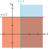
FIGURE 8.4.4Solution The set in Example 3
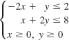
EXAMPLE 4 System of Linear Inequalities
Graph the system of linear inequalities
![]()
Solution Substitution of (0, 0) into the first inequality in (4) gives the true statement 0 ≤ 1, which implies that the graph of the solutions of x + y ≤ 1 is the half-plane below(and including) the line x + y = 1. This is the shaded blue region in Figure 8.4.5(a). Similarly, substituting (0, 0) into the second inequality gives the false statement 0 ≥ 4, and so the graph of the solutions of –x + 2y ≥ 4 is the half-plane above (and including) the line –x + 2y = 4. This is the shaded red region in Figure 8.4.5(b). The graph of the solutions of the system of inequalities is then the intersection of the graphs of these two solution sets. This intersection is the darker region of overlapping colors shown in Figure 8.4.5(c).
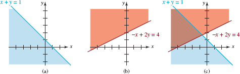
FIGURE 8.4.5Solution set in Example 4
Often we are interested in the solutions of a system of linear inequalities subject to the restrictions that x ≥ 0 and y ≥ 0. This means that the graph of the solutions is a subset of the set consisting of the points in the first quadrant and on the nonnegative coordinate axes. For example, inspection of Figure 8.4.5(c) reveals that the system of inequalities (4) subject to the added requirements that x ≥ 0, y ≥ 0, has no solutions.
EXAMPLE 5 System of Linear Inequalities
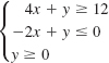
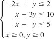
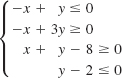
The graph of the solutions of the system of linear inequalities
![]()
is the region shown in Figure 8.4.6(a). The graph of the solutions of
is the region in the first quadrant along with portions of the two lines and portions of the coordinate axes illustrated in Figure 8.4.6(b).
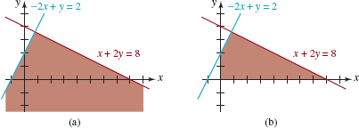
FIGURE 8.4.6Solution set in Example 5
![]() Nonlinear Inequalities Graphing nonlinear inequalities in two variables x and y is basically the same as graphing linear inequalities. In the next example we again utilize the notion of a test point.
Nonlinear Inequalities Graphing nonlinear inequalities in two variables x and y is basically the same as graphing linear inequalities. In the next example we again utilize the notion of a test point.
EXAMPLE 6 Graph of a Nonlinear Inequality
To graph the nonlinear inequality
![]()
we begin by drawing the circle x2 + y2 = 4 using a solid line. Since (0, 0) lies in the interior of the circle we can use it for a test point. Substituting x = 0 and y = 0 in the inequality gives the false statement -4 ≥ 0 and so the solution set of the given inequality consists of all the points either on the circle or in its exterior. See FIGURE 8.4.7.
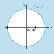
FIGURE 8.4.7Solution set in Example 6
EXAMPLE 7 System of Inequalities
Graph the system of inequalities
![]()
Solution Substitution of the coordinates of (0, 0) into the first inequality gives the true statement 0 ≤ 4 and so the graph of y ≤ 4 – x2 is the shaded blue region in FIGURE 8.4.8 below the parabola y = 4 - x2. Note that we cannot use (0, 0) as a test point for the second inequality since (0, 0) is a point on the line y = x. However, if we use (1, 2) as a test point, the second inequality gives the true statement 2 > 1. Thus the graph of the solutions of y > x is the shaded red half-plane above the line y = x in FIGURE 8.4.8. The line itself is dashed because of the strict inequality. The intersection of these two colored regions is the darker region in the figure.

FIGURE 8.4.8 Solution set in Example 7
8.4Exercises: Answers to selected odd-numbered problems begin on page ANS-20.,
In Problems 1-12, graph the given inequality.
x + 3y ≥ 6
x – y ≤ 4
x + 2y < –x + 3y
2x + 5y > x – y + 6
–y ≥ 2(x + 3) – 5
x ≥ 3(x + 1) + y
y ≥ (x – 1)2
![]()
![]()
![]()
y ≥ | x + 2 |
xy ≥ 3
In Problems 13–36, graph the given system of inequalities.
![]()
![]()
![]()
![]()

![]()
![]()


![]()
![]()
![]()
![]()
![]()

![]()
![]()


In Problems 37–40, find a system of linear inequalities whose graph is the region shown in the figure.
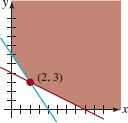
FIGURE 8.4.9Region for Problem 37
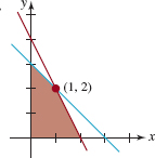
FIGURE 8.4.10Region for Problem 38
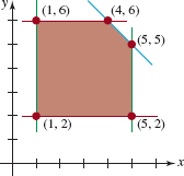
FIGURE 8.4.11Region for Problem 39
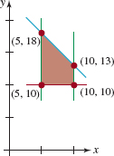
FIGURE 8.4.12Region for Problem 40
For Discussion
In Problems 41 and 42, graph the given inequality.
–1 ≤ x + y ≤ 1
–x ≤ y ≤ x
Project
Ancient History and USPS Some years ago the restrictions on first-class envelope size were a bit more confusing than they are today. Consider the rectangular envelope of length x and height y shown in FIGURE 8.4.13 and the following postal regulation of November 1978:
All first-class items weighing one ounce or less and all single-piece third-class items weighing two ounces or less are subject to an extra mailing fee when the height is greater than 6
in., or the length is greater than 11
in., or the length is less than 1.3 times the height, or the length is greater than 2.5 times the height.
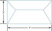
FIGURE 8.4.13 Envelope in Problem 43
In parts (a)–(c) assume that the weight specification is satisfied.
(a) Using x and y, interpret the above regulation as a system of linear inequalities.
(b) Graph the region that describes envelope sizes that are not subject to an extra mailing fee.
(c) Under this regulation does an envelope of length 8 in. and height 4 in. require an extra fee?
(d) Do some research and compare the 2010 first class regulation against the one just given.
8.5 Linear Programming
![]() Introduction A linear function in two variables is a function of the form
Introduction A linear function in two variables is a function of the form
![]()
where a, b, and c are constants, with a domain a subset of the Cartesian plane. The basic problem in linear programming is to find the maximum (largest) value or the minimum (smallest) value of a linear function that is defined on a set determined by a system of linear inequalities. In this section we will discuss a way of finding a maximum or minimum value of F.
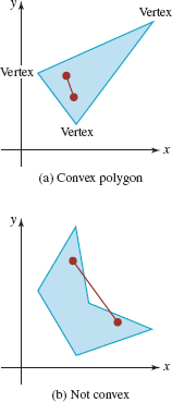
FIGURE 8.5.1Polygons in the plane
![]() Terminology A typical linear-programming problem is given by
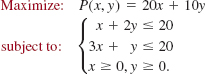
Terminology A typical linear-programming problem is given by
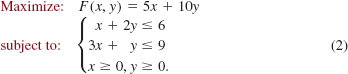
In this context, F is called the objective function and the linear inequalities are called constraints. Any ordered pair of real numbers (x0, y0) that satisfies all the constraints is said to be a feasible solution of the problem. The set of feasible solutions will be denoted by S. It can be shown that for any two points in the graph of S, the line segment joining them lies entirely in the graph. Any set in the plane having this property is called convex. Figure 8.5.1(a) illustrates a convex polygon; Figure 8.5.1(b) illustrates a polygon that is not convex. The corner points of the convex set S determined by the constraints are called vertices.
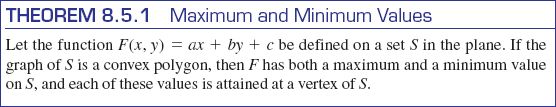
Throughout this discussion we will be concerned with the graph of the set S of feasible solutions of a system of linear inequalities in which x ≥ 0 and y ≥ 0.We state the following theorem without proof.
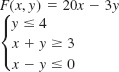
EXAMPLE 1 Finding Max and Min Values
Find the maximum and minimum values of the objective function in (2).
Solution We first graph the set S of feasible solutions and find all vertices by solving the appropriate simultaneous equations. For example, the vertex ![]() is obtained by solving the system of equations:
is obtained by solving the system of equations:
![]()
See FIGURE 8.5.2. It follows from Theorem 8.5.1 that the maximum and minimum values of F occur at vertices. From the accompanying table, we see that the maximum value of the objective function is
![]()
The minimum value is F(0, 0) = 0.
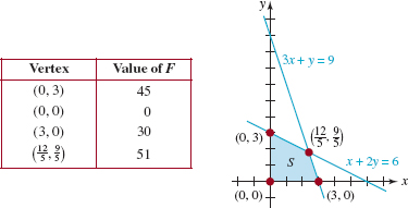
FIGURE 8.5.2Convex set for Example 1
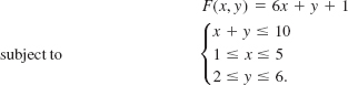
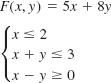
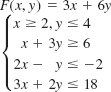
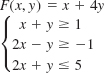
EXAMPLE 2 Finding Max and Min Values
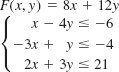
Find the maximum and minimum values of
Solution In FIGURE 8.5.3 the graph of S determined by the constraints is given and the vertices are labeled. As we see from the accompanying table, the maximum value of F is
![]()
The minimum value is
![]()
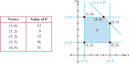
FIGURE 8.5.3Convex set for Example 2
EXAMPLE 3 Maximum Profit
A small tool manufacturing company has two forges F1 and F2 each of which, because of maintenance requirements, can operate at most 20 h per day. The company makes two types of tools, A and B. Tool A must spend 1 h in forge F1 and 3 h in forge F2. Tool B must spend 2 h in forge F1 and 1 h in forge F2. The company makes a $20 profit on tool A and a $10 profit on tool B. Determine the number of each type of tool the company must make in order to maximize its daily profit.
Solution Let
x = the number of tools A produced each day, and
y = the number of tools B produced each day.
The objective function is the daily profit
![]()
The total number of hours per day that both tools spend in forge F1 must satisfy
![]()
Similarly, the total number of hours per day that both tools spend in forge F2 must satisfy
![]()
Thus we wish to
The graph of S determined by the constraints is shown in FIGURE 8.5.4. From the table accompanying FIGURE 8.5.4, we see that the maximum daily profit is
![]()
That is, when the company makes four of tool A and eight of tool B each day, its maximum daily profit is $160.
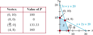
FIGURE 8.5.4Convex set for Example 3
EXAMPLE 4 Minimum Cost
In his spare time John does piecework at home making pairs of mittens, scarfs, and stocking caps. During the winter he produces a total of 300 of these items per month. He has a standing monthly order at a large outdoor mail-order company for 50 to 100 pairs of mittens, for at least 100 scarfs, and for at least 70 stocking caps. The costs of the material used are $0.20 for each pair of mittens, $0.40 for each scarf, and $0.50 for each stocking cap. Determine the number of each item that should be made each month in order to minimize his monthly total cost.
Solution Let x and y denote the number of pairs of mittens and scarfs, respectively, supplied by John to the mail-order company each month. The number of stocking caps supplied each month is then 300 – x – y. The objective function is the total monthly costs
![]()
The constraints are
The last inequality in this system of inequalities is equivalent to x + y ≤ 230. The graph of the S of feasible solutions determined by the constraints and the vertices of the set is shown in FIGURE 8.5.5. From the accompanying table, we see that C(100, 300) = 107 is the minimum. Thus John should make 100 pairs of mittens, 130 scarfs, and 70 stocking caps each month in order to minimize his total costs.
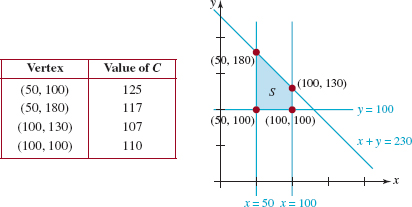
FIGURE 8.5.5Convex set for Example 4
You should not get the impression from the preceding discussion that an objective function must have both a maximum and a minimum. If the graph of S is not a convex polygon, then the conclusion of Theorem 8.5.1 may not be true. Depending on the constraints, it could happen that a linear function F has a minimum but no maximum (or vice versa). However, it can be shown that if F has a minimum (or a maximum) on S, then it is attained at a vertex of the region. Also, the maximum (or minimum) of an objective function may occur at more than one vertex.
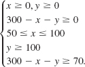
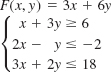
EXAMPLE 5 Minimum but No Maximum
Consider the linear function
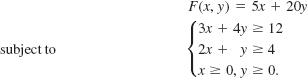
Inspection of FIGURE 8.5.6 shows that the graph of the set S of the solutions of the constraints is not a convex polygon. It can be proved that
![]()
is a minimum. However, in this case, the objective function has no maximum since F(x, y) can be increased without bound simply by increasing x(x ≥ 4) or by increasing y(y ≥ 4).
FIGURE 8.5.6Convex set for Example 5
8.5Exercises: Answers to selected odd-numbered problems begin on page ANS-21.
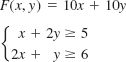
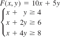
In Problems 1–12, find the maximum and minimum values of the given linear function F on the set S defined by the constraints. In each problem assume that x ≥ 0and y ≥ 0.

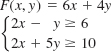
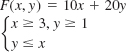
In Problems 13–16, the given objective function F subject to the constraints has a minimum value. Find this value. Explain why F has no maximum value. Assume that x ≥ 0 and y ≥ 0.
Miscellaneous Applications
How Many? A company manufactures satellite radios and portable DVD players. It makes a $10 profit on each radio and a $40 profit on a DVD player. Due to limited production facilities, the total number of radios and DVD players that the company can manufacture in one month is at most 350. Because of the availability of parts, the company can manufacture at most 300 radios and 100 DVD players each month. Determine how many satellite radios and DVD players the company should produce each month in order to maximize its profit.
Making Money A woman has up to $10,000 that she wishes to invest in two kinds of certificates of deposit, A and B, that return, respectively, 6.5% and 7.5% annually. She wants to invest at most three times as much in B as in A. Find the maximum annual return if no more than $6000 can be invested in B and no more than $5000 in A.
Out-of-Pocket Cost A patient is informed that her daily intake of vitamins must be at least 6 units of A, 4 units of B, and 18 units of C, but no more than 12 units of A, 8 units of B, and 56 units of C. She finds that a drugstore sells two brands, X and Y, of multiple vitamins containing the necessary vitamins. One capsule of brand X contains 1 unit of A, 1 unit of B, and 7 units of C, and costs 5 cents. One capsule of brand Y contains 3 units of A, 1 unit of B, and 2 units of C, and costs 6 cents. How may capsules of each brand should the patient take each day in order to minimize her cost?

How much of each?
Cost of Doing Business An insurance company uses two computers, an IBC 490 and a CDM 500. Each hour the IBC can process 8 units (1 unit = 1000) of medical claims, 1 unit of life insurance claims, and 2 units of car insurance claims. Each hour the CDM can process 2 units of medical claims, 1 unit of life insurance claims, and 7 units of car insurance claims. The company finds it necessary to process at least 16 units of medical claims, at least 5 units of life insurance claims, and at least 20 units of car insurance claims per day. If it costs the company $100 an hour to run the IBC and $200 an hour to run the CDM, at most how many hours should each computer be run each day in order to keep the company's cost per day at a minimum? What is the minimum cost? Is there a maximum cost per day?
Making a Profit Kerry's Warehouse has a supply of 1300 pairs of designer jeans and 1700 pairs of generic-brand jeans, which are to be shipped out to two stores: an upscale location and a discount outlet. The warehouse receives a profit of $14.25 per pair on the designer jeans and $12.50 per pair on the generic-brand jeans at the upscale location. The corresponding profits at the discount outlet are $4.80 and $3.40 per pair. The upscale location, however, can carry at most 1800 pairs of jeans, whereas the discount outlet has room for at most 2500 pairs. Find the number of pairs of both designer jeans and generic-brand jeans that the warehouse should ship to each store in order to maximize its total profit. What is the maximum profit?
Minimize the Cost Joan's manufacturing company makes three kinds of custom sports cars; A, B, and C. Her company turns out a total of 100 cars each year. The number of B cars made must not exceed three times the number of A cars made, but their combined yearly production must be at least 20. The number of C cars made each year must be at least 32. Each A car costs $9000 to build. The B and C cars cost $6000 and $8000, respectively. How many of each kind of car should be built in order to minimize the company's yearly production cost? What is the minimum cost?

Moose eating aquatic plants
A Healthy Diet Moose living in a national park in Michigan eat both aquatic plants, which are high in sodium but low in energy content (they contain a lot of water), and terrestrial plants, which are high in energy content but contain essentially no sodium. Experiments have shown that a moose can get about 0.8 mj (megajoules) of energy from 1 kg of aquatic plants and about 3.2 mj of energy from 1 kg of terrestrial plants. It has been estimated that an adult moose needs to eat at least 17 kg of aquatic plants daily in order to satisfy its sodium needs. It has also been estimated that the moose rumen (the first stomach) is incapable of digesting more than 33 kg of food daily. Find the daily intakes of both aquatic and terrestrial plants that will maximize a moose's energy intake, subject to its sodium requirement and rumen capacity.
Chapter 8Review Exercises: Answers to selected odd-numbered problems begin on page ANS-21.
A. True/False__________________________________________________
In Problems 1–10, answer true or false.
The graphs of 2x + 7y = 6 and x4 + 8xy – 3y6 = 0 intersect at (–4, 2).____
The homogeneous system
possesses only the zero solution (0, 0, 0).____
The system
![]()
always has two solutions when m ≠ 0 and k > 0.____
The system
![]()
has no solution.____
The nonlinear systems
![]()
are equivalent.____
(1, –2) is a solution of the inequality 4x – 3y + 5 ≤ 0.____
The origin is in the half-plane determined by 4x – 3y < 6.____
The system of inequalities
![]()
has no solutions._____
The system of nonlinear equations
![]()
has exactly three solutions.____
The form of the partial fraction decomposition of ![]() is
is
![]()
B. Fill in the Blanks_____________________________________________
In Problems 1–10, fill in the blanks.
The system
![]()
is ___________(consistent or inconsistent).
The system
![]()
is consistent for b =___________
The graph of a single linear inequality in two variables represents a ___________in the plane.
In words, describe the graph of the inequality 1 ≤ x – y ≤ 4.___________
To decompose
![]()
into partial fractions we begin with___________
The solution of the system
is___________.
If the system of two linear equations in two variables has an infinite number of solutions, then the equations are said to be___________.
If the graph of y = ax2 + bx passes through (1, 1) and (2, 1), then a = ___________ and b = ___________.
The graph of the system

lies in the ___________ quadrant.
A system of inequalities whose graph is given in Figure 8.R.1 is ___________.
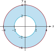
FIGURE 8.R.1Graph for Problem 10
C. Review Exercises_____________________________________________
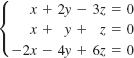
In Problems 1–14, solve the given system of equations.
![]()
![]()
![]()

![]()
![]()
![]()
![]()
![]()
![]()
![]()
Playing with Numbers In a two-digit number, the units digit is 1 greater than 3 times the tens digit. When the digits are reversed, the new number is 45 more than the old number. Find the old number.
Lengths A right triangle has an area of 24 cm2. If its hypotenuse has a length of 10 cm, find the lengths of the remaining two sides of the triangle.
Got a Wire Cutter? A wire 1 m long is cut into two pieces. One piece is bent into a circle and the other piece is bent into a square. The sum of the areas of the circle and the square is ![]() m2. What are the length of the side of the square and the radius of the circle?
m2. What are the length of the side of the square and the radius of the circle?
Coordinates Find the coordinates of the point P of intersection of the line and the parabola shown in Figure 8.R.2.
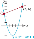
FIGURE 8.R.2Graphs for Problem 18
In Problems 19–22, find the partial fraction decomposition of the given rational expression.
![]()
![]()
![]()
![]()
In Problems 23–28, graph the given system of inequalities.


![]()
![]()
In Problems 29–32, use the functions y = x2 and y = 2 – x to form a system of inequalities whose graph is given in the figure.

FIGURE 8.R.3Graph for Problem 29
FIGURE 8.R.4Graph for Problem 30
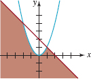
FIGURE 8.R.5Graph for Problem 31

FIGURE 8.R.6Graph for Problem 32
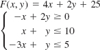
Find the maximum and minimum values of
![]()
subject to
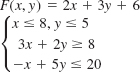
The function F(x, y) = 20x + 5y subject to the constraints

has a minimum value. What is it? Explain why the function has no maximum value.
Total Return On a certain small farm, farming an acre of corn requires 6 h of labor and $36 of capital, whereas farming an acre of oats requires 2 h of labor and $18 of capital. Suppose the farmer has 12 acres of land, 48 h of labor, and $360 of capital available. If the return on the corn is $40 per acre and on oats is $20 per acre, how many acres of each should the farmer plant in order to maximize the total return (including unused capital)?