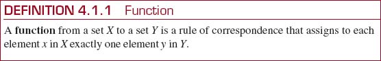
4 Functions and Graphs

In This Chapter

4.1 Functions and Graphs

4.2 Symmetry and Transformations

4.3 Linear and Quadratic Functions

4.4 Piecewise-Defined Functions

4.5 Combining Functions

4.6 Inverse Functions

4.7 Building a Function from Words

4.8 Least Squares Line

Chapter 4 Review Exercises

The correspondence between the students in a class and the set of desks filled by these students is an example of a function.

A Bit of History If the question “What is the most important mathematical concept?” were posed to a group of mathematicians, mathematics teachers, and scientists, certainly the term function would appear near or even at the top of the list of their responses. In Chapters 4 and 5, we will focus primarily on the definition and the graphical interpretation of a function.

The word function was probably introduced by the German mathematician and “co-inventor” of calculus, Gottfried Wilhelm Leibniz (1646-1716), in the late seventeenth century and stems from the Latin word functo, meaning to act or perform. In the seventeenth and eighteenth centuries, mathematicians had only the most intuitive notion of a function. To many of them, a functional relationship between two variables was given by some smooth curve or by an equation involving the two variables. Although formulas and equations play an important role in the study of functions, we will see in Section 4.1 that the “modern” interpretation of a function (dating from the middle of the nineteenth century) is that of a special type of correspondence between the elements of two sets.

4.1 Functions and Graphs

Introduction Using the objects and the persons around us, it is easy to make up a rule of correspondence that associates, or pairs, the members, or elements, of one set with the members of another set. For example, to each social security number there is a person, to each car registered in the state of California there is a license plate number, to each book there corresponds at least one author, to each state there is a governor, and so on. A natural correspondence occurs between a set of 20 students and a set of, say, 25 desks in a classroom when each student selects and sits in a different desk. In mathematics we are interested in a special type of correspondence, a single-valued correspondence, called a function.

The set Y is not necessarily the range

In the student/desk correspondence above suppose the set of 20 students is the set X and the set of 25 desks is the set Y. This correspondence is a function from the set X to the set Y provided no student sits in two desks at the same time.

Terminology A function is usually denoted by a letter such as f, g, or h. We can then represent a function f from a set X to a set Y by the notation f: X → Y. The set X is called the domain of f. The set of corresponding elements y in the set Y is called the range of the function. For our student/desk function, the set of students is the domain and the set of 20 desks actually occupied by the students constitutes the range. Notice that the range of f need not be the entire set Y. The unique element y in the range that corresponds to a selected element x in the domain X is called the value of the function at x, or the image of x, and is written f(x). The latter symbol is read “f of x” or “f at x,” and we write y = f(x). See FIGURE 4.1.1. In many texts, x is also called the input of the function f and the value f(x) is called the output of f. Since the value of y depends on the choice of x, y is called the dependent variable; x is called the independent variable. Unless otherwise stated, we will assume hereafter that the sets X and Y consist of real numbers.

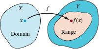
FIGURE 4.1.1 Domain and range of a function f

EXAMPLE 1 The Squaring Function

The rule for squaring a real number is given by the equation y = x² or f(x) = x². The values of f at x = –5 and x = are obtained by replacing x, in turn, by the numbers -5 and :

Occasionally for emphasis we will write a function using parentheses in place of the symbol x. For example, we can write the squaring function f(x) = x² as

This illustrates the fact that x is a placeholder for any number in the domain of the function y = f(x). Thus, if we wish to evaluate (1) at, say, 3 + h, where h represents a real number, we put 3 + h into the parentheses and carry out the appropriate algebra:

If a function f is defined by means of a formula or an equation, then typically the domain of y = f(x) is not expressly stated. We will see that we can usually deduce the domain of y = f(x) either from the structure of the equation or from the context of the problem.

EXAMPLE 2 Domain and Range

In Example 1, since any real number x can be squared and the result x² is another real number, f(x) = x² is a function from R to R, that is, f: R → R. In other words, the domain of f is the set R of real numbers. Using interval notation, we also write the domain as (-∞,∞). The range of f is the set of nonnegative real numbers or [0,∞); this follows from the fact that x² ≥ 0 for every real number x.

Domain of a Function As mentioned earlier, the domain of a function y = f(x) that is defined by a formula is usually not specified. Unless stated or implied to the contrary, it is understood that

The domain of a function f is the largest subset of the set of real numbers for which f(x) is a real number.

This set is sometimes referred to as the implicit domain of the function. For example, we cannot compute f (0) for the reciprocal function f(x) = 1/x since 1/0 is not a real number. In this case we say that f is undefined at x = 0. Since every nonzero real number has a reciprocal, the domain of f(x) = 1/x is the set of real numbers except 0. By the same reasoning, the function g(x) = 1/(x² – 4) is not defined at either x = – 2 or x = 2, and so its domain is the set of real numbers with the numbers – 2 and 2 excluded. The square root function h(x) = is not defined at x = – because is not a real number. In order for h(x) = to be defined in the real number system we must require the radicand, in this case simply x, to be non-negative. From the inequality x ≥ 0 we see that the domain of the function h is the interval [0,∞;).

EXAMPLE 3 Domain and Range

Determine the domain and range of

Solution The radicand x – 3 must be nonnegative. By solving the inequality x – 3 ≥ 0 we get x ≥ 3, and so the domain of f is [3,∞). Now, since the symbol denotes the principal square root of a number, for x ≥ 3 and consequently The smallest value of f(x) occurs at x = 3 and is f (3) = 4 + = 4. Moreover, because x – 3 and – 3 increase as x takes on increasingly larger values, we conclude that y ≥ 4. Consequently the range of f is [4, ∞).

EXAMPLE 4 Domain of f

Determine the domain of

Solution As in Example 3, the expression under the radical symbol—the radicand— must be nonnegative; that is, the domain of f is the set of real numbers x for which x² + 2x – 15 ≥ 0 or (x – 3)(x + 5) ≥ 0. We have already solved the last inequality by means of a sign chart in Example 1 of Section 2.7. The solution set of the inequality (–∞, –5] U [3,∞)is the domain of f.

EXAMPLE 5 Domains of Two Functions

Determine the domain of and

Solution A function that is given by a fractional expression is not defined at the x-values for which its denominator is equal to 0.

(a) The expression under the radical is the same as in Example 4. Since x² + 2x – 15 is in the denominator we must have x² + 2x – 15 ≠ 0. This excludes x = – 5 and x = 3. In addition, since x² + 2x – 15 appears under a radical, we must have x² + 2x – 15 > 0 for all other values of x. Thus the domain of the function g is the union of two open intervals (–∞, – 5) U (3,∞).

(b) Since the denominator of h(x) factors, x² – 3x – 4 = (x + 1)(x – 4), we see that (x + 1)(x – 4) = 0for x = – 1 and x = 4. In contrast to the function in part (a), these are the only numbers for which h is not defined. Hence, the domain of the function h is the set of real numbers with x = – 1 and x = 4 excluded.

Using interval notation, the domain of the function h in part (b) of Example 5 can be written as

As an alternative to this ungainly union of disjoint intervals, this domain can also be written using set-builder notation as

Graphs A function is often used to describe phenomena in fields such as science, engineering, and business. In order to interpret and utilize data, it is useful to display this data in the form of a graph. The graph of a function f is the graph of the set of ordered pairs (x, f(x)), where x is in the domain of f. In the xy-plane an ordered pair (x, f(x)) is a point, so that the graph of a function is a set of points. If a function is defined by an equation y = f(x), then the graph of f is the graph of the equation. To obtain points on the graph of an equation y = f(x), we judiciously choose numbers x₁, x₂, x₃,…in its domain, compute f(x₁), f(x₂), f(x₃),…, plot the corresponding points (x₁, f(x₁)), (x₂, f(x₂)), (x₃, f(x₃)),…and then connect these points with a curve. See FIGURE 4.1.2. Keep in mind that

a value of x is a directed distance from the y-axis, and

a function value f(x) is a directed distance from the x-axis.

FIGURE 4.1.2 Points on the graph of an equation y = f(x)

End Behavior A word about the figures in this text is in order. With a few exceptions, it is usually impossible to display the complete graph of a function, and so we often display only the more important features of the graph. In FIGURE 4.1.3(a), notice that the graph goes down on its left and right sides. Unless indicated to the contrary, we may assume that there are no major surprises beyond what we have shown and the graph simply continues in the manner indicated. The graph in Figure 4.1.3(a) indicates the so-called end behavior or global behavior of the function: For a point (x, y) on the graph, the values of the y-coordinate become unbounded in magnitude in the downward or negative direction as the x-coordinate becomes unbounded in magnitude in both the negative and positive directions on the number line. It is convenient to describe this end behavior using the symbols

The arrow symbol → in (2) is read “approaches.” Thus, for example, y → –∞ as x → ∞ is read “y approaches negative infinity as x approaches infinity.”

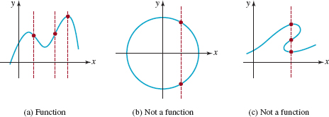
FIGURE 4.1.3 Vertical line test

More will be said about this concept of global behavior in Chapter 005. If a graph terminates at either its right or left end, we will indicate this by a dot when clarity demands it. See FIGURE 4.1.4. We will use a solid dot to represent the fact that the endpoint is included on the graph and an open dot to signify that the endpoint is not included on the graph.

FIGURE 4.1.4 Domain and range interpreted graphically

Vertical Line Test From the definition of a function we know that for each x in the domain of f there corresponds only one value f(x) in the range. This means a vertical line that intersects the graph of a function y = f(x) (this is equivalent to choosing an x) can do so in at most one point. Conversely, if every vertical line that intersects a graph of an equation does so in at most one point, then the graph is the graph of a function. The last statement is called the vertical line test for a function. See Figure 4.1.3(a). On the other hand, if some vertical line intersects a graph of an equation more than once, then the graph is not that of a function. See Figures 3.1.3(b) and 3.1.3(c). When a vertical line intersects a graph in several points, the same number x corresponds to different values of y in contradiction to the definition of a function.

If you have an accurate graph of a function y = f(x), it is often possible to see the domain and range of f. In FIGURE 4.1.4 assume that the colored curve is the entire, or complete, graph of some function f. The domain of f then is the interval [a, b] on the x-axis and the range is the interval [c, d] on the y-axis.

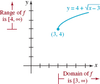
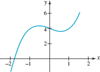
FIGURE 4.1.5 Graph of function f in Example 6

EXAMPLE 6 Example 3 Revisited

From the graph of f(x) = 4 + given in FIGURE 4.1.5, we can see that the domain and range of f are, respectively, [3, ∞) and [4, ∞). This agrees with the results in Example 3.

As shown in Figure 4.1.3(b), a circle is not the graph of a function. Actually, an equation such as x² + y² = 9 defines (at least) two functions of x. If we solve this equation for y in terms of x we get Because of the single-valued convention for the symbol, both equations and define functions. As we saw in Section 3.2, the first equation defines an upper semicircle and the second defines a lower semicircle. From the graphs shown in FIGURE 4.1.6, the domain of is [–3, 3] and the range is [0, 3]; the domain and range of are [–3, 3] and [–3, 0], respectively.

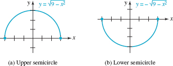
FIGURE 4.1.6 These semicircles are graphs of functions

Intercepts To graph a function defined by an equation y = f(x), it is usually a good idea to first determine whether the graph of f has any intercepts. Recall that all points on the y-axis are of the form (0, y). Thus, if 0 is in the domain of a function f, the y-intercept is the point on the y-axis whose y-coordinate is f(0), in other words, (0, f (0)). See FIGURE 4.1.7(a). Similarly, all points on the x-axis have the form (x, 0). This means that to find the x-intercepts of the graph of y = f(x), we determine the values of x that make y = 0. That is, we must solve the equation f(x) = 0 for x. A number c for which

is referred to as either a zero of the function f or a root (or solution) of the equation f(x) = 0. The real zeros of a function f are the x-coordinates of the x-intercepts of the graph of f. In Figure 4.1.7(b), we have illustrated a function that has three zeros x₁, x₂, and x₃ because f(x₁) = 0, f(x₂) = 0, and f(x₃) = 0. The corresponding three x-intercepts are the points (x₁, 0), (x₂, 0), and (x₃, 0). Of course, the graph of the function may have no intercepts. This is illustrated in FIGURE 4.1.5.

FIGURE 4.1.7 Intercepts of the graph of a function f

A graph does not necessarily have to cross a coordinate axis at an intercept, a graph could simply be tangent to, or touch, an axis. In Figure 4.1.7(c) the graph of y = f(x) is tangent to the x-axis at (x₁, 0). Also, the graph of a function f can have at most one y-intercept since, if 0 is the domain of f, there can correspond only one y-value, namely, y = f(0).

EXAMPLE 7 Intercepts

Find, if possible, the x- and y-intercepts of the given function.

(a) (b)

Solution (a) Since 0 is in the domain of f, f(0) = – 2 is the y-coordinate of the y-intercept of the graph of f. The y-intercept is the point (0, – 2). To obtain the x-intercepts we must determine whether f has any real zeros, that is, real solutions of the equation f(x) = 0. Since the left-hand side of the equation x² + 2x – 2 = 0 has no obvious factors, we use the quadratic formula to obtain . Since the zeros of f are the numbers 1 – and 1 + . The x-intercepts are the points (1 – , 0) and (1 + , 0).

(b) Because 0 is not in the domain of f(f(0) = – 3/0 is not defined), the graph of f possesses no y-intercept. Now since f is a fractional expression, the only way we can have f(x) = 0 is to have the numerator equal zero. Factoring the left-hand side of x² – 2x – 3 = 0 gives (x + 1)(x – 3) = 0. Therefore the numbers –1 and 3 are the zeros of f. The x-intercepts are the points (–1, 0) and (3, 0).

Approximating Zeros Even when it is obvious that the graph of a function y = f(x) possesses x-intercepts it is not always a straightforward matter to solve the equation f(x) = 0. In fact, it is impossible to solve some equations exactly; sometimes the best we can do is to approximate the zeros of the function. One way of doing this is to obtain a very accurate graph of f.

EXAMPLE 8 Intercepts

With the aid of a graphing utility the graph of the function f(x) = x³ – x + 4 is given in FIGURE 4.1.8. From f(0) = 4 we see that the y-intercept is (0, 4). As we see in the figure, there appears to be only one x-intercept with its x-coordinate close to –1.7 or –1.8. But there is no convenient way of finding the exact values of the roots of the equation x³ – x + 4 = 0. We can, however, approximate the real root of this equation with the aid of the find root feature of either a graphing calculator or computer algebra system. We find that x ≈ –1.796 and so the approximate x-intercept is (-1.796, 0).As a check, note that the function value

FIGURE 4.1.8 Approximate x-intercept in Example 8

is nearly 0.

NOTES FROM THE CLASSROOM

When sketching the graph of a function, you should never resort to plotting a lot of points by hand. That is something a graphing calculator or a computer algebra system (CAS) does so well. On the other hand, you should not become dependent on a calculator to obtain a graph. Believe it or not, there are instructors who do not allow the use of graphing calculators on quizzes or tests. Usually there is no objection to your using calculators or computers as an aid in checking homework problems, but in the classroom instructors want to see the product of your own mind, namely, the ability to analyze. So you are strongly encouraged to develop your graphing skills to the point where you are able to quickly sketch by hand the graph of a function from a basic familiarity of types of functions and by plotting a minimum of well-chosen points, and by using the transformations introduced in the next section.

4.1 Exercises Answers to selected odd-numbered problems begin on page ANS-7.

In Problems 1–6, find the indicated function values.

1. If and f(6)

2.If and f(7)

3. If and f(5)

4. If and f(4)

5. If and f()

6. If and f(½)

In Problems 7 and 8, find

for the given function f and simplify as much as possible.

7. f( ) = –2( )² + 3( )

8. f( ) = ( )³ – 2( )² + 20

9. For what values of x is f(x) = 6x² – 1 equal to 23?

10. For what values of x is equal to 4?

In Problems 11–20, find the domain of the given function f.

11.

12.

13.

14.

15.

16.

17.

18.

19.

20.

In Problems 21–26, use the sign-chart method to find the domain of the given function f.

21.

22.

23.

24.

25.

26.

In Problems 27–30, determine whether the graph in the figure is the graph of a function.

27.

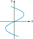
FIGURE 4.1.9 Graph for Problem 27

28.

FIGURE 4.1.10 Graph for Problem 28

29.

FIGURE 4.1.11 Graph for Problem 29

30.

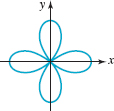
FIGURE 4.1.12 Graph for Problem 30

In Problems 31–34, use the graph of the function f given in the figure to find its domain and range.

31.

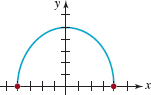
FIGURE 4.1.13Graph for Problem 31

32.

FIGURE 4.1.14Graph for Problem 32

33.

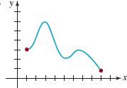
FIGURE 4.1.15Graph for Problem 33

34.

FIGURE 4.1.16Graph for Problem 34

In Problems 35–42, find the zeros of the given function f.

35.

36.

37.

38.

39.

40.

41.

42.

In Problems 43–50, find the x– and y–intercepts, if any, of the graph of the given function f. Do not graph.

43.

44.

45.

46.

47.

48.

49.

50.

In Problems 51 and 52, find two functions y = f₁(x) and y = f₂(x) defined by the given equation. Find the domain of the functions f₁ and f₂.

51.

52.

In Problems 53 and 54, use the graph of the function f given in the figure to estimate the values of f(– 3), f(– 2), f(–1), f(1), f(2), and f(3). Estimate the y-intercept.

53.

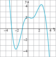
FIGURE 4.1.17Graph for Problem 53

54.

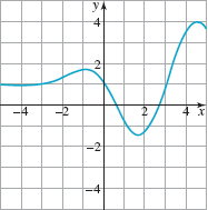
FIGURE 4.1.18Graph for Problem 54

In Problems 55 and 56, use the graph of the function f given in the figure to estimate the values of f(–2),f(–1.5),f(0.5),f(1),f(2), and f(3.2). Estimate the x-intercepts.

55.

FIGURE 4.1.18Graph for Problem 55

56.

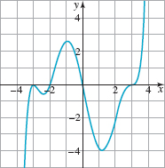
FIGURE 4.1.18Graph for Problem 56

57. Factorial Function In your study of mathematics some of the functions that you will encounter have as their domain the set of positive integers n. The factorial function f(n) = n! is defined as the product of the first n positive integers, that is,

(a) Evaluate f(2),f(3),f(5), and f(7).

(b) Show that f(n + 1) = f(n) · (n + 1).

(c) Simplify f(n + 2)/f(n).

58. A Sum Function Another function of a positive integer n gives the sum of the first n squared positive integers:

(a) Find the value of the sum 1² + 2² +…+ 99² + 100².

(b) Find n such that 300 < S(n) < 400. [Hint: Use a calculator.]

For Discussion

59. Determine an equation of a function y = f (x) whose domain is (a) [3, ∞), (b) (3, ∞).

60. Determine an equation of a function y = f(x) whose range is (a) [3, ∞), (b) (3, ∞).

61. What is the only point that can be both an x- and a y-intercept for the graph of a function y = f(x)?

62. Consider the function After factoring the denominator and canceling a common factor we can write Discuss: Is x = 1 in the domain of ?

4.2 Symmetry and Transformations

Introduction In this section we discuss two aids in sketching graphs of functions quickly and accurately. If you determine in advance that the graph of a function possesses symmetry, then you can cut your work in half. In addition, sketching a graph of a complicated-looking function is expedited if you recognize that the required graph is actually a transformation of the graph of a simpler function. This latter graphing aid is based on your prior knowledge of the graphs of some basic functions.

Power Functions A function of the form

where n represents a real number is called a power function. The domain of a power function depends on the power n. For example, we have already seen in Section 4.1 for n = 2, n = ½, and n = –1, respectively, that

the domain of f(x) = x² is the set R of real numbers or (–∞, ∞),

the domain of f(x) = x½ = is [0, ∞), and

the domain of is the set R of real numbers except x = 0.

Simple power functions, or modified versions of these functions, occur so often in problems that you do not want to spend valuable time plotting their graphs. We suggest that you know (memorize) the short catalogue of graphs of power functions given in FIGURE 4.2.1. You already know that the graph in part (a) of that figure is a line and may know that the graph in part (b) is called a parabola.

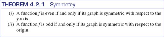
Symmetry In Section 3.2 we discussed symmetry of a graph with respect to the y-axis, the x-axis, and the origin. Of those three types of symmetries, the graph of a function can be symmetric with respect to the y-axis or with respect to the origin, but the graph of a nonzero function cannot be symmetric with respect to the x-axis. See Problem 43 in Exercises 4.2. If the graph of a function is symmetric with respect to the y-axis, then as we know the points (x, y) and (–x, y) are on the graph of f. Similarly, if the graph of a function is symmetric with respect to the origin, the points (x, y) and (–x, –y) are on its graph. For functions, the following two tests for symmetry are equivalent to tests (i) and (ii), respectively, on page 136.

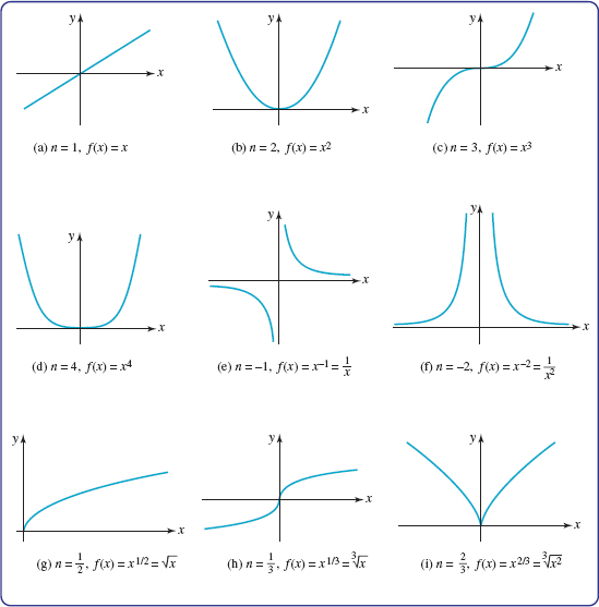
FIGURE 4.2.1 Brief catalogue of power functions f(x) = xⁿ for various n

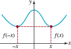
FIGURE 4.2.2 Even function

In FIGURE 4.2.2, observe that if f is an even function and

is also on its graph. Similarly we see in FIGURE 4.2.3 that if f is an odd function and

is on its graph. We have proved the following result.

FIGURE 4.2.3 Odd function

Inspection of Figures 3.2.2 and 3.2.3 shows that the graphs, in turn, are symmetric with respect to the y-axis and origin. The function whose graph is given in FIGURE 4.2.4 is neither even nor odd, and so its graph possesses no y-axis or origin symmetry.

In view of Definition 4.2.1 and Theorem 4.2.1 we can determine symmetry of a graph of a function in an algebraic manner.

Function is neither odd nor even

EXAMPLE 1 Odd and Even Functions

(a) f(x) = x³ is an odd function since by Definition 4.2.1(ii),

This proves what we see in Figure 4.2.1(c), the graph of f(x) = x³ is symmetric with respect to the origin. For example, since f(1) = 1,(1, 1) is a point on the graph of y = x³. Because f is an odd function, f (– 1) = –f (1) implies (–1, –1) is on the same graph.

(b) f (x) = x^2/3is an even function since by Definition 4.2.1(i) and the laws of exponents

In Figure 4.2.1(i), we see that the graph of f is symmetric with respect to the y-axis. For example, since f(8) = 8 = 4, (8, 4) is a point on the graph of y = x. Because f is an even function, f (–8) = f(8) implies (–8, 4) is also on the same graph.

(c) f(x) = x³ + 1 is neither even nor odd. From

we see that f(–x) ≠ f(x), and f(–x) ≠ –f(x). Hence the graph of f is neither symmetric with respect to the y-axis nor symmetric with respect to the origin.

The graphs in FIGURE 4.2.1, with part (g) the only exception, possess either y-axis or origin symmetry. The functions in Figures 3.2.1(b), (d), (f), and (i) are even, whereas the functions in Figures 3.2.1(a), (c), (e), and (h) are odd.

Often we can sketch the graph of a function by applying a certain transformation to the graph of a simpler function (such as those given in FIGURE 4.2.1). We will consider two kinds of graphical transformations, rigid and nonrigid.

Rigid Transformations A rigid transformation of a graph is one that changes only the position of the graph in the xy-plane but not its shape. For example, the circle (x – 2)² + (y – 3)² = 1 with center (2, 3) and radius r = 1, has exactly the same shape as the circle x² + y² = 1 with center at the origin. Thus we can think of the graph of (x – 2)² + (y – 3)² = 1 as the graph of x² + y² = 1 shifted horizontally 2 units to the right followed by an upward vertical shift of 3 units. For the graph of a function y = f(x) we examine four kinds of shifts or translations.

Consider the graph of a function y = f(x) given in FIGURE 4.2.5. The shifts of this graph described in (i)–(iv) of Theorem 4.2.2 are the graphs in red in parts (a)–(d) of FIGURE 4.2.6. If (x, y) is a point on the graph of y = f(x) and the graph of f is shifted, say, upward by c > 0 units, then (x, y + c) is a point on the new graph. In general, the x-coordinates do not change as a result of a vertical shift. See Figures 3.2.6(a) and 3.2.6(b). Similarly, in a horizontal shift the y-coordinates of points on the shifted graph are the same as on the original graph. See Figures 3.2.6(c) and 3.2.6(d).

FIGURE 4.2.5 Graph of y = f(x)

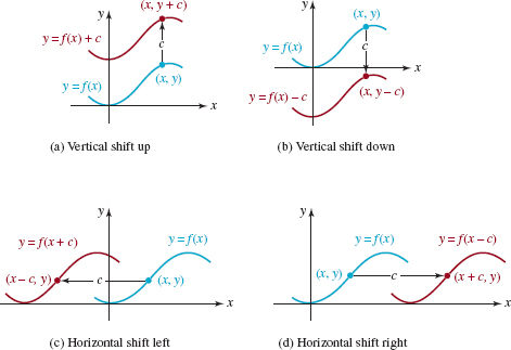
FIGURE 4.2.6 Vertical and horizontal shifts of the graph of y = f(x) by an amount c > 0.

EXAMPLE 2 Vertical and Horizontal Shifts

The graphs of y = x² + 1, y = x² – 1, y = (x + 1)², and y = (x – 1)² are obtained from the blue graph of f(x) = x² in Figure 4.2.7(a) by shifting this graph, in turn, 1 unit up (Figure 4.2.7(b)), 1 unit down (Figure 4.2.7(c)), 1 unit to the left (Figure 4.2.7(d)), and 1 unit to the right (Figure 4.2.7(e)).

FIGURE 4.2.7 Shifted graphs in red in Example 2

Combining Shifts In general, the graph of a function

where c₁ and c₂ are positive constants, combines a horizontal shift (left or right) with a vertical shift (up or down). For example, the graph of y = f(x – c₁) + c₂ is the graph of y = f(x) shifted c₁ units to the right and then c₂ units up.

EXAMPLE 3 Graph Shifted Horizontally and Vertically

Graph y = (x+ 1)² – 1.

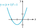
FIGURE 4.2.8 Shifted graph in Example 3

Solution From the preceding paragraph we identify in (3) the form y = f(x + c₁) – c₂ with c₁ = 1 and c₂ = 1.Thus, the graph of y = (x + 1)² – 1 is the graph of f(x) = x² shifted 1 unit to the left followed by a downward shift of 1 unit. The graph is given in FIGURE 4.2.8.

From the graph in FIGURE 4.2.8 we see immediately that the range of the function y = (x + 1)² – 1 = x² + 2x is the interval [–1, ∞) on the y-axis. Note also that the graph has x-intercepts (0, 0) and (–2, 0); you should verify this by solving x² + 2x = 0. Also, if you reexamine FIGURE 4.1.5 in Section 4.1 you will see that the graph of y = 4 + is the graph of the square root function f(x) = (Figure 3.2.1(g)) shifted 3 units to the right and then 4 units up.

Another way of rigidly transforming a graph of a function is by a reflection in a coordinate axis.

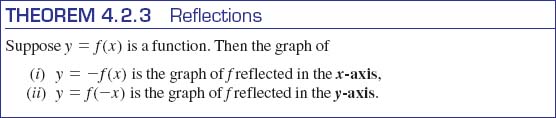
In part (a) of FIGURE 4.2.9 we have reproduced the graph of a function y = f(x) given in FIGURE 4.2.5. The reflections of this graph described in parts (i) and (ii) of Theorem 4.2.3 are illustrated in Figures 3.2.9(b) and 3.2.9(c). If (x, y) denotes a point on the graph of y = f(x), then the point (x, –y) is on the graph of y = –f(x) and (–x, y) is on the graph of y = f(–x). Each of these reflections is a mirror image of the graph of y = f(x) in the respective coordinate axis.

Reflection or mirror image

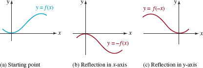
FIGURE 4.2.9 Reflections in the coordinate axes

EXAMPLE 4 Reflections

Graph

(a) y = –

(b) y =

Solution The starting point is the graph of f(x) = given in Figure 4.2.10(a).

(a) The graph of y = – is the reflection of the graph of f(x) = in the x-axis. Observe in Figure 4.2.10(b) that since (1, 1) is on the graph of f, the point (1, – 1) is on the graph of y = – .

(b) The graph of y = is the reflection of the graph of f(x) = in the y-axis. Observe in Figure 4.2.10(c) that since (1, 1) is on the graph of f, the point (– 1, 1) is on the graph of y = . The function y = looks a little strange, but bear in mind that its domain is determined by the requirement that – x ≥ 0, or equivalently x ≤ 0, and so the reflected graph is defined on the interval (– ∞, 0].

FIGURE 4.2.10 Reflected graphs in red in Example 4

If a function f is even, then f(–x) = f(x) shows that a reflection in the y-axis would give precisely the same graph. If a function is odd, then from f(–x) = –f(x) we see that a reflection of the graph of f in the y-axis is identical to the graph of f reflected in the x-axis. In FIGURE 4.2.11 theblue curve is the graph of the odd function f(x) = x³; the red curve is the graph of y = f(–x) = (–x)³ = –x³. Notice that if the blue curve is reflected in either the y-axis or the x-axis, we get the red curve.

FIGURE 4.2.11 Reflection of an odd function in y-axis

Nonrigid Transformations If a function f is multiplied by a constant c > 0, the shape of the graph is changed but retains, roughly, its original shape. The graph of y = cf(x) is the graph of y = f(x) distorted vertically; the graph of f is either stretched (or elongated) vertically or is compressed (or flattened) vertically depending on the value of c. Stretching or compressing a graph are examples of nonrigid transformations.

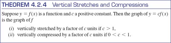
FIGURE 4.2.12Vertical stretch of the graph of f (x) = x

If (x, y) represents a point on the graph of f, then the point (x, cy) is on the graph of cf. The graphs of y = x and y = 3x are compared in FIGURE 4.2.12; the y-coordinate of a point on the graph of y = 3x is 3 times as large as the y-coordinate of the point with the same x-coordinate on the graph of y = x. The comparison of the graphs of y = 10x²(blue graph) and (red graph) in FIGURE 4.2.13 is a little more dramatic; the graph of exhibits considerable vertical flattening, especially in a neighborhood of the origin. Note that c is positive in this discussion. To sketch the graph of y = – 10x² we think of it as y = – (10x²), which means we first stretch the graph of y = x² vertically by a factor of 10 units, and then reflect that graph in the x-axis.

The next example illustrates shifting, reflecting, and stretching of a graph.

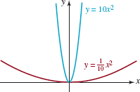
FIGURE 4.2.13 Vertical stretch (blue) and vertical compression (red) of the graph of f(x) = x²

EXAMPLE 5 Combining Transformations

Graph y = 2 – 2 .

Solution You should recognize that the given function consists of four transformations of the basic function f(x) = :

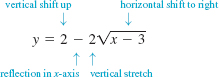
We start with the graph of f(x) = in Figure 4.2.14(a). Then stretch this graph vertically by a factor of 2 to obtain y = 2 in Figure 4.2.14(b). Reflect this second graph in the x-axis to obtain y = –2 in Figure 4.2.14(c). Shift this third graph 3 units to the right to obtain y = –2 in Figure 4.2.14(d). Finally, shift the fourth graph upward 2 units to obtain y = 2 – 2 in Figure 4.2.14(e). Note that the point (0, 0) on the graph of f(x) = remains fixed in the vertical stretch and the reflection in the x-axis, but under the first (horizontal) shift (0, 0) moves to (3, 0) and under the second (vertical) shift (3, 0) moves to (3, 2).

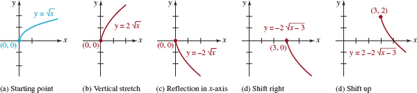
FIGURE 4.2.14 Graph of y = 2 – 2 in Example 5 is given in part (e)

4.1 Exercises Answers to selected odd–numbered problems begin on page ANS-7.

In Problems 1–10, use (1) and (2) to determine whether the given function y = f(x) is even, odd, or neither even nor odd. Do not graph.

1.

2.

3.

4.

5.

6.

7.

8.

9.

10.

In Problems 11–14, classify the function y = f(x) whose graph is given as even, odd, or neither even nor odd.

11.

FIGURE 4.2.15Graph for Problem 11

12.

FIGURE 4.2.16Graph for Problem 12

13.

FIGURE 4.2.17Graph for Problem 13

14.

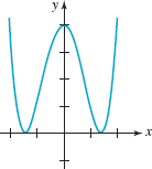
FIGURE 4.2.18Graph for Problem 14

In Problems 15–18, complete the graph of the given function y = f(x) if (a) f is an even function and (b) f is an odd function.

15.

FIGURE 4.2.19Graph for Problem 15

16.

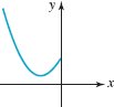
FIGURE 4.2.20Graph for Problem 16

17.

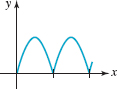
FIGURE 4.2.21Graph for Problem 17

18.

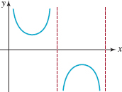
FIGURE 4.2.22Graph for Problem 18

In Problems 19 and 20, suppose that f(—2) = 4 and f(3) = 7. Determine f(2) and f(–3)

19. If f is an even function

20. If f is an odd function

In Problems 21 and 22, suppose that g(–1) = –5 and g(4) = 8. Determine g(1) and g (—4).

21. If g is an odd function

22. If g is an even function

In Problems 23–32, the points (–2, 1) and (3, –4) are on the graph of the function y = f (x). Find the corresponding points on the graph obtained by the given transformations.

23. The graph of f shifted up 2 units

24. The graph of f shifted down 5 units

25. The graph of f shifted to the left 6 units

26. The graph of f shifted to the right 1 unit

27. The graph of f shifted up 1 unit and to the left 4 units

28. The graph of f shifted down 3 units and to the right 5 units

29. The graph of f reflected in the y-axis

30. The graph of f reflected in the x-axis

31. The graph of f stretched vertically by a factor of 15 units

32. The graph of f compressed vertically by a factor of unit, then reflected in the x-axis

In Problems 33–36, use the graph of the function y = f (x) given in the figure to graph the following functions

(a) y = f(x) + 2

(b) y = f(x) – 2

(c) y = f(x + 2)

(d) y = f(x – 5)

(e) y = –f(x)

(f) y = f(–x)

33.

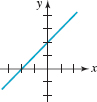
FIGURE 4.2.23Graph for Problem 33

34.

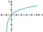
FIGURE 4.2.24Graph for Problem 34

35.

FIGURE 4.2.25Graph for Problem 35

36.

FIGURE 4.2.26Graph for Problem 36

In Problems 37 and 38, use the graph of the function y = f(x) given in the figure to graph the following functions

(a) y = f(x) + 1

(b) y = f(x) – 1

(c) y = f(x + π)

(d)

(e) y = –f(x)

(f) y = f(–x)

(g) y = 3f(x)

(h)

37.

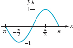
FIGURE 4.2.27Graph for Problem 37

38.

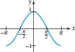
FIGURE 4.2.28Graph for Problem 38

In Problems 39–42, find the equation of the final graph after the given transformations are applied to the graph of y = f(x).

39. The graph of f(x) = x³ shifted up 5 units and right 1 unit

40. The graph of f(x) = x stretched vertically by a factor of 3 units, then shifted right 2 units

41. The graph of f(x) = x⁴ reflected in the x-axis, then shifted left 7 units

42. The graph of f(x) = 1/x reflected in the y-axis, then shifted left 5 units and down 10 units

For Discussion

43. Explain why the graph of a function y = f(x) cannot be symmetric with respect to the x-axis.

44. What points, if any, on the graph of y = f(x) remain fixed, that is, the same on the resulting graph after a vertical stretch or compression? After a reflection in the x-axis? After a reflection in the y-axis?

45. Discuss the relationship between the graphs of y = f(x) and

46. Discuss the relationship between the graphs of y = f(x) and y = f(cx), where c > 0 is a constant. Consider two cases: 0 < c < 1 and c > 1.

47. Review the graphs of y = x and y = 1/x in FIGURE 4.2.1. Then discuss how to obtain the graph of the reciprocal function y = 1/f(x) from the graph of y = f(x). Sketch the graph of y = 1/f (x) for the function f whose graph is given in FIGURE 4.2.26.

48. In terms of transformations of graphs, describe the relationship between the graph of the function y = f(cx), c a constant, and the graph of y = f (x). Consider two cases c > 1 and 0 < c < 1. Illustrate your answers with several examples.

4.3 Linear and Quadratic Functions

Introduction When n is a nonnegative integer, the power function f(x) = xⁿ is just a special case of a class of functions called polynomial functions. A polynomial function is a function of the form

where n is a nonnegative integer. The three functions considered in this section, are polynomial functions. In the definitions that follow we change the coefficients of these functions to more convenient symbols.

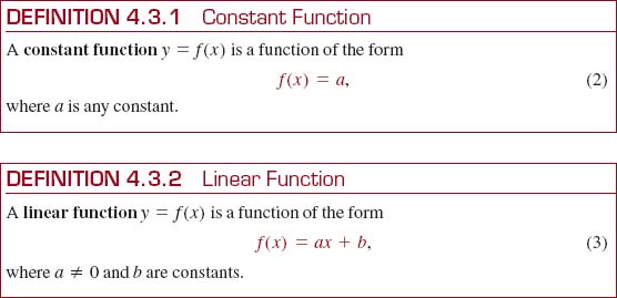
In the form y = a we know from Section 3.3 that the graph of a constant function is simply a horizontal line. Similarly, when written as y = ax + b we recognize a linear function as the slope–intercept form of a line with the symbol a playing the part of the slope m. Hence the graph of every linear function is a nonhorizontal line with slope. The domain of a constant function as well as a linear function is the set of real numbers (–∞, ∞).

The squaring function y = x² that played an important role in Section 4.2 is a member of a family of functions called quadratic functions.

Graphs The graph of any quadratic function is called a parabola. The graph of a quadratic function has the same basic shape of the squaring function y = x² shown in FIGURE 4.3.1. In the examples that follow we will see that the graphs of quadratic functions f(x) = ax² + bx + c are simply transformations of the graph of y = x²:

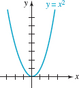
FIGURE 4.3.1 Graph of simplest parabola

The graph of f(x) = ax², a > 0, is the graph of y = x² stretched vertically when a > 1, and compressed vertically when 0 < a < 1.

The graph of f(x) = ax², a < 0, is the graph of y = ax², a > 0, reflected in the x-axis.

The graph of f(x) = ax² + bx + c, b ≠ 0, is the graph of y = ax² shifted horizontally or vertically.

From the first two items in the bulleted list, we conclude that the graph of a quadratic function opens upward (as in FIGURE 4.3.1) if a > 0 and opens downward if a < 0.

EXAMPLE 1 Stretch, Compression, and Reflection

(a) The graphs of y = 4x² and are, respectively, a vertical stretch and a vertical compression of the graph of y = x². The graphs of these functions are shown in Figure 4.3.2(a); the graph of y = 4x² is shown in red, the graph of is green, and the graph of y = x² is blue.

(b) The graphs of y = –4x², and y = –x² are obtained from the graphs of the functions in part (a) by reflecting their graphs in the x-axis. See Figure 4.3.2(b).

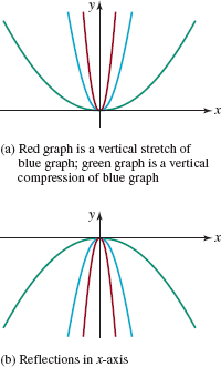
FIGURE 4.3.2 Graphs of quadratic functions in Example 1

Vertex and Axis If the graph of a quadratic function opens upward a > 0 (or downward a < 0), the lowest (highest) point (h, k) on the parabola is called its vertex. All parabolas are symmetric with respect to a vertical line through the vertex (h, k). The line x = h is called the axis of symmetry or simply the axis of the parabola. See FIGURE 4.3.3.

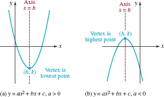
FIGURE 4.3.3Vertex and axis of a parabola

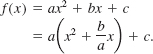
Standard Form The vertex of a parabola can be determined by recasting the equation f(x) = ax² + bx + c into the standard form

The form (5) is obtained from the equation (4) by completing the square in x. Recall, completing the square in (4) starts with factoring the number a from all terms involving the variable x:

Within the parentheses we add and subtract the square of one-half the coefficient of x:

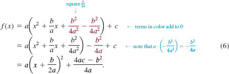
The last expression is equation (5) with the identifications h = –b/2a and k = (4ac – b²)/4a. If a > 0, then necessarily a(x – h)² ≥ 0. Hence f(x) in (5) is a minimum when (x – h)² = 0, that is, for x = h. A similar argument shows that if a < 0 in (5), f(x) is a maximum value for x = h. Thus (h, k) is the vertex of the parabola. The equation of the axis of the parabola is x = h or x = –b/2a.

We strongly suggest that you do not memorize the result in the last line of (6), but practice completing the square each time. However, if memorization is permitted by your instructor to save time, then the vertex can also be found by computing the coordinates of the point

Intercepts The graph of (4) always has a y-intercept since 0 is in the domain of f. From f(0) = c we see that the y-intercept of a quadratic function is (0, c). To determine whether the graph has x-intercepts we must solve the equation f(x) = 0. The last equation can be solved either by factoring or by using the quadratic formula. Recall, a quadratic equation ax² + bx + c = 0, a ≠ 0, has the solutions

We distinguish three cases according to the algebraic sign of the discriminant b² – 4ac.

If b² – 4ac > 0, then there are two distinct real solutions x₁ and x₂. The parabola crosses the x-axis at (x₁, 0) and (x₂, 0).

If b² – 4ac = 0, then there is a single real solution x₁. The vertex of the parabola is located on the x-axis at (x₁, 0). The parabola is tangent to, or touches, the x-axis at this point.

If b² – 4ac < 0, then there are no real solutions. The parabola does not cross the x-axis.

As the next example shows, a reasonable sketch of a parabola can be obtained by plotting the intercepts and the vertex.

EXAMPLE 2 Graph Using Intercepts and Vertex

Graph f(x) = x² – 2x – 3.

Solution Since a = 1 > 0 we know that the parabola will open upward. From f(0) = –3 we get the y-intercept (0, –3). To see whether there are any x-intercepts we solve x² – 2x – 3 = 0. By factoring,

we find the real solutions x = –1, x = 3 and so the x-intercepts are (–1, 0) and (3, 0). To locate the vertex we complete the square:

Thus the standard form is f(x) = (x – 1)² – 4. With the identifications h = 1 and k = –4, we conclude that the vertex is (1, –4). Using this information we draw a parabola through these four points as shown in FIGURE 4.3.4.

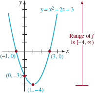
FIGURE 4.3.4 Parabola in Example 2

One last observation. By finding the vertex we automatically determine the range of a quadratic function. In our current example, y = –4 is the smallest number in the range of f and so the range of f is the interval [–4, ∞) on the y-axis.

EXAMPLE 3 Vertex Is the x-intercept

Graph f(x) = –4x² + 12x – 9.

Solution The graph of this quadratic function is a parabola that opens downward because a = –4 < 0. To complete the square we start by factoring –4 from the two x-terms:

FIGURE 4.3.5 Parabola in Example 3

Thus the standard form is . With h = and k = 0 we see that the vertex is (, 0). The y-intercept is (0,f(0)) = (0, –9). Solving – 4x² + 12x – 9 = –4(x – )² = 0, we see that there is only one x-intercept, namely, (, 0). Of course, this was to be expected because the vertex (, 0) is on the x-axis. As shown in FIGURE 4.3.5 a rough sketch can be obtained from these two points alone. The parabola is tangent to the x-axis at (, 0).

EXAMPLE 4 Using (7) to Find the Vertex

Graph f(x) = x² + 2x + 4.

Solution The graph is a parabola that opens upward because a = 1 > 0.For the sake of illustration we will use (7) this time to find the vertex. With b = 2, –b/2a = –2/2 = – 1 and

the vertex is (– 1, f(– 1)) = (–1, 3). Now the y-intercept is (0,f(0)) = (0, 4) but the quadratic formula shows that the equation f(x) = 0 or x² + 2x + 4 = 0 has no real solutions. Therefore the graph has no x-intercepts. Since the vertex is above the x-axis and the parabola opens upward, the graph must lie entirely above the x-axis. See FIGURE 4.3.6.

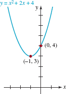
FIGURE 4.3.6 Parabola in Example 4

Graphs by Transformations The standard form (5) clearly describes how the graph of any quadratic function is constructed from the graph of y = x² starting with a non-rigid transformation followed by two rigid transformations:

y = ax² is the graph of y = x² stretched or compressed vertically.

y = a(x – h)² is the graph of y = ax² shifted |h| units horizontally.

y = a(x – h)² + k is the graph of y = a(x – h)² shifted |k| units vertically.

FIGURE 4.3.7 illustrates the horizontal and vertical shifting in the case where a > 0, h > 0, and k > 0.

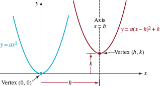
FIGURE 4.3.7 The red graph is obtained by shifting the blue graph h units to the right and k units upward.

EXAMPLE 5 Horizontally Shifted Graphs

Compare the graphs of (a) y = (x – 2)² and (b) y = (x + 3)².

Solution The blue dashed graph in FIGURE 4.3.8 is the graph of y = x². Matching the given functions with (6) shows in each case that a = 1 and k = 0. This means that neither graph undergoes a vertical stretch or a compression, and neither graph is shifted vertically.

(a) With the identification h = 2, the graph of y = (x – 2)² is the graph of y = x² shifted horizontally 2 units to the right. The vertex (0, 0) for y = x² becomes the vertex (2, 0) for y = (x – 2)². See the red graph in FIGURE 4.3.8.

(b) With the identification h = –3, the graph of y = (x + 3)² is the graph of y = x² shifted horizontally |–3| = 3 units to the left. The vertex (0, 0) for y = x² becomes the vertex (–3, 0) for y = (x + 3)². See the green graph in FIGURE 4.3.8.

FIGURE 4.3.8 Shifted graphs in Example 5

EXAMPLE 6 Shifted Graph

Graph y = 2(x – 1)² – 6.

Solution The graph is the graph of y = x² stretched vertically upward, followed by a horizontal shift to the right of 1 unit, followed by a vertical shift downward of 6 units. In FIGURE 4.3.9 you should note how the vertex (0, 0) on the graph of y = x² is moved to (1, –6) on the graph of y = 2(x – 1)² – 6 as a result of these transformations. You should also follow by transformations how the point (l, l) shown in Figure 4.3.9(a) ends up as (2, –4) in Figure 4.3.9(d).

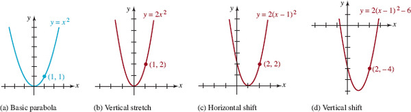
FIGURE 4.3.9 Graphs in Example 6

Graphical Solution of Inequalities Graphs can be of help in solving certain inequalities when a sign chart is not useful because the quadratic does factor conveniently. For example, the quadratic function in Example 6 is equivalent to y = 2x² – 4x – 4. Were we required to solve the inequality 2x² – 4x – 4 ≥ 0 we see in Figure 4.3.9(d) that y ≥ 0 to the left of the x-intercept on the negative x-axis and to the right of the x-intercept on the positive x-axis. The x-coordinates of these intercepts, obtained by solving 2x² – 4x – 4 = 0 by the quadratic formula are 1 – and 1 + . Thus the solution of 2x² – 4x – 4 ≥ 0 is the union of intervals (–∞, 1 – ] U [1 + , ∞).

FIGURE 4.3.10 Function f is increasing on [a, b] in (a); is decreasing on [a, b] in (b)

Increasing–Decreasing Functions We have seen in Figures 3.3.2(a) and 3.3.2(b) that if a > 0 (which, as we have just seen plays the part of m), the values of a linear function f(x) = ax + b increase as x-increases, whereas for a < 0, the values f(x) decrease as x increases. The notions of increasing and decreasing can be extended to any function. The ability to determine intervals over which a function f is either increasing or decreasing plays an important role in applications of calculus.

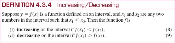
In Figure 4.3.10(a) the function f is increasing on the interval [a, b], whereas f is decreasing on [a, b] in Figure 4.3.10(b). A linear function f(x) = ax + b, increases on the interval (-∞, ∞) for a > 0 and decreases on the interval (-∞, ∞) for a < 0. Similarly, if a > 0, then the quadratic function f in (5) is decreasing on the interval (–∞, h] and increasing on the interval [h, ∞).If a < 0, we have just the opposite, that is, f is increasing on (–∞, h] followed by decreasing on [h, ∞). Reinspection of FIGURE 4.3.6 shows that f(x) = x² + 2x + 4 is decreasing on the interval (–∞, –1] and increasing on the interval [–1,∞). In general, if h is the x-coordinate of the vertex of a quadratic function f, then f changes either from increasing to decreasing or from decreasing to increasing at x = h. For this reason, the vertex (h, k) of the graph of a quadratic function is also called a turning point for the graph of f.

Freely Falling Object In rough terms, an equation or a function that is constructed using certain assumptions about some real-world situation or phenomenon with the intent to describe that phenomenon is said to be a mathematical model. Suppose an object, such as a ball, is either thrown straight upward (downward) or simply dropped from an initial height s₀. Then if the positive direction is taken to be upward, a mathematical model for the height s(t) of the object aboveground is given by the quadratic function

where g is the acceleration due to gravity (-39 ft/s² or -9.8 m/s²), v₀ is the initial velocity imparted to the object, and t is time measured in seconds. See FIGURE 4.3.11. If the object is dropped, then v₀ = 0. An assumption in the derivation of (10) is that the motion takes place close to the surface of the Earth and so the retarding effect of air resistance is ignored. Also, the velocity of the object while it is in the air is given by the linear function

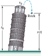
FIGURE 4.3.11 Rock thrown upward from an initial height s₀

See Problems 59–69 in Exercises 4.3.

4.3 Exercises Answers to selected odd-numbered problems begin on page ANS-8.

In Problems 1 and 2, find a linear function (3) that satisfies both of the given conditions.

1. f(–1) = 5, f(1) = 6

2. f(–1) = 1 + f(2), f(3) = 4f(1)

In Problems 3–6, find the point of intersection of the graphs of the given linear functions. Sketch both lines.

3. f(x) = –2x + 1, g(x) = 4x + 6

4. f(x) = 2x + 5, g(x) = x + 5

5.

6. f(x) = 2x – 10, g(x) = –3x

In Problems 7–12, for the given function compute the quotient where h is a constant.

7.

8.

9.

10.

11.

12.

In Problems 13–18, sketch the graph of the given quadratic function f.

13. f(x) = 2x²

14. f(x) = -2x²

15. f(x) = 2x² - 2

16. f(x) = 2x² + 5

17. f(x) = -2x² + 1

18. f(x) = -2x² - 3

In Problems 19–30, consider the quadratic function f.

(a) Find all intercepts of the graph of f.

(b) Express the function f in standard form.

(c) Find the vertex and axis of symmetry.

(d) Sketch the graph of f.

19. f(x) = x(x + 5)

20. f(x) = -x² + 4x

21. f(x) = (3 - x)(x + 1)

22. f(x) = (x - 2)(x - 6)

23. f(x) = x² - 3x + 2

24. f(x) = -x² + 6x - 5

25. f(x) = 4x² - 4x + 3

26. f(x) = -x² + 6x - 10

27. f(x) = -½ x² + x + 1

28. f(x) = x² - 2x - 7

29. f(x) = x² - 10x + 25

30. f(x) = -x² + 6x - 9

In Problems 31 and 32, find the maximum or the minimum value of the function f. Give the range of the function f.

31. f(x) = 3x² - 8x + 1

32. f(x) = - 2x² - 6x + 3

In Problems 33–36, find the largest interval on which the function f is increasing and the largest interval on which f is decreasing.

33. f(x) = x² – 25

34. f(x) = – (x + 10)²

35. f(x) = –2x² – 12x

36. f(x) = x² + 8x – 1

In Problems 37–42, describe in words how the graph of the given function f can be obtained from the graph of y = x² by rigid or nonrigid transformations.

37. f(x) = (x – 10)²

38. f(x) = (x + 6)²

39. f(x) = - (x + 4)² + 9

40. f(x) = 10(x – 2)² – 1

41. f(x) = (–x – 6)² – 4

42. f(x) = – (1 – x)² + 1

In Problems 43–48, the given graph is the graph of y = x² shifted/reflected in the xy-plane. Write an equation of the graph.

43.

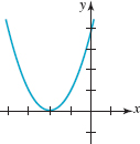
FIGURE 4.3.12 Graph for Problem 43

44.

FIGURE 4.3.13 Graph for Problem 44

45.

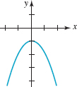
FIGURE 4.3.14 Graph for Problem 45

46.

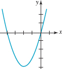
FIGURE 4.3.15 Graph for Problem 46

47.

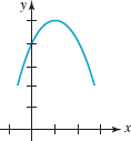
FIGURE 4.3.16 Graph for Problem 47

48.

FIGURE 4.3.17 Graph for Problem 48

In Problems 49 and 50, find a quadratic function f(x) = ax² + bx + c that satisfies the given conditions.

49. f has the values f(0) = 5,f(1) = 10, and f(–1) = 4

50. Graph passes through (2, –1), zeros of f are 1 and 3

In Problems 51 and 52, find a quadratic function in standard form f(x) = a(x – h)² + k that satisfies the given conditions.

51. The vertex of the graph of f is (1, 2), graph passes through (2, 6)

52. The maximum value of f is 10, axis of symmetry is x = –1, and y-intercept is (0, 8)

In Problems 53–56, sketch the region in the xy-plane that is bounded between the graphs of the given functions. Find the points of intersection of the graphs.

53. y = – x + 4, y = x² + 2x

54. y = 2x — 2, y = 1 – x²

55. y = x² + 2x + 2, y = –x² – 2x + 2

56. y = x² – 6x + 1, y = –x² + 2x + 1

57. (a) Express the square of the distance d from the point (x, y) on the graph of y = 2x to the point (5, 0) shown in FIGURE 4.3.18 as a function of x.

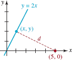
FIGURE 4.3.18 Distance in Problem 57

(b) Use the function in part (a) to find the point (x, y) that is closest to (5, 0).

Miscellaneous Applications

58. Shooting an Arrow As shown in FIGURE 4.3.19, an arrow that is shot at a 45° angle with the horizontal travels along a parabolic arc defined by the equation y = a x² + x + c. Use the fact that the arrow is launched at a vertical height of 6 ft and travels a horizontal distance of 200 ft to find the coefficients a and c. What is the maximum height attained by the arrow?

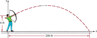
FIGURE 4.3.19 Arrow in Problem 58

59. Shooting Another Arrow An arrow is shot vertically upward with an initial velocity of 64 ft/s from a point 6 ft above the ground. See FIGURE 4.3.20.

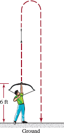
FIGURE 4.3.20Arrow in Problem 59

(a) Find the height s(t) and the velocity v(t) of the arrow at time t ≥ 0.

(b) What is the maximum height attained by the arrow? What is the velocity of the arrow at the time the arrow attains its maximum height?

(c) At what time does the arrow fall back to the 6-ft level? What is its velocity at this time?

60. How High The height above ground of a toy rocket launched upward from the top of a building is given by s(t) = – 16t² + 96t + 256.

(a) What is the height of the building?

(b) What is the maximum height attained by the rocket?

(c) Find the time when the rocket strikes the ground.

61. Impact Velocity A ball is dropped from the roof of a building that is 122.5 m above ground level.

(a) What is the height and velocity of the ball at t = 1 s?

(b) At what time does the ball hit the ground?

(c) What is the impact velocity of the ball when it hits the ground?

62. A True Story, but… A few years ago a newspaper in the Midwest reported that an escape artist was planning to jump off a bridge into the Mississippi River wearing 70 lb of chains and manacles. The newspaper article stated that the height of the bridge was 48 ft and predicted that the escape artist's impact velocity on hitting the water would be 85 mi/h. Assuming that he simply dropped from the bridge, then his height (in feet) and velocity (in feet/second) t seconds after jumping off the bridge are given by the functions s(t) = —16t² + 48 and v(t) = –32t, respectively, determine whether the newspaper's estimate of his impact velocity was accurate.

63. Thermometers The functional relationship between degrees Celsius T_C and degrees Fahrenheit T_F is linear.

(a) Express T_F as a function of T_C if (0°C, 32°F) and (60°C, 140°F) are on the graph of T_F.

(b) Show that 100°C is equivalent to the Fahrenheit boiling point 212°F. See FIGURE 4.3.21.

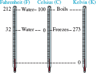
FIGURE 4.3.21 Thermometers in Problems 63 and 64

64. Thermometers—Continued The functional relationship between degrees Celsius T_C and temperatures measured in kelvin units T_K is linear.

(a) Express T_K as a function of T_C if (0°C, 273 K) and (27°C, 300 K) are on the graph of T_K.

(b) Express the boiling point 100°C in kelvin units. See FIGURE 4.3.21.

(c)Absolute zero is defined to be 0 K. What is 0 K in degrees Celsius?

(d)Express T_K as a linear function of T_F.

(e) What is 0 K in degrees Fahrenheit?

65. Simple Interest In simple interest, the amount A accrued over time is the linear function A = P + P_rt, where P is the principal, t is measured in years, and r is the annual interest rate (expressed as a decimal). Compute A after 20 years if the principal is P = $1000, and the annual interest rate is 3.4%. At what time is A = $2200?

66. Linear Depreciation Straight line, or linear, depreciation consists of an item losing all its initial worth of A dollars over a period of n years by an amount A/n each year. If an item costing $20,000 when new is depreciated linearly over 25 years, determine a linear function giving its value V after x years, where 0 ≤ x ≤ 25. What is the value of the item after 10 years?

67. Spread of a Disease One mathematical model for the spread of a flu virus assumes that within a population of P persons the rate at which a disease spreads is jointly proportional to the number D of persons already carrying the disease and the number P – D of persons not yet infected. Mathematically, the model is given by the quadratic function

Spreading a virus

where R(D) is the rate of spread of the flu virus (in cases per day) and k > 0 is a constant of proportionality.

(a) Show that if the population P is a constant, then the disease spreads most rapidly when exactly one–half the population is carrying the flu.

(b) Suppose that in a town of 10,000 persons, 125 are sick on Sunday, and 37 new cases occur on Monday. Estimate the constant k.

(c) Use the result of part (b) to estimate the number of new cases on Tuesday. [Hint: The number of persons carrying the flu on Monday is 162 = 125 + 37.]

(d) Estimate the number of new cases on Wednesday, Thursday, Friday, and Saturday.

For Discussion

68. Consider the linear function If x is changed by 1 unit, how many units will y change? If x is changed by 2 units? If x is changed by n (n a positive integer) units?

69. Consider the interval [x₁, x₂] and the linear function f(x) = ax + b, a ≠ 0. Show that

and interpret this result geometrically for a > 0.

70. In Problems 60 and 62, what is the domain of the function s(t)? [Hint: It is not (–∞, ∞).]

71. On the Moon the acceleration due to gravity is one-sixth the acceleration due to gravity on Earth. If a ball is tossed vertically upward from the surface of the Moon, would it attain a maximum height six times that on Earth when the same initial velocity is used? Defend your answer.

72. Suppose the quadratic function f(x) = ax² + bx + c has two distinct real zeros. How would you prove that the x-coordinate of the vertex is the midpoint of the line segment between the x-coordinates of the intercepts? Carry out your ideas.

4.4 Piecewise-Defined Functions

Introduction A function f may involve two or more expressions or formulas, with each formula defined on different parts of the domain of f. A function defined in this manner is called a piecewise-defined function. For example,

is not two functions, but a single function in which the rule of correspondence is given in two pieces. In this case, one piece is used for the negative real numbers (x < 0) and the other part for the nonnegative real numbers (x ≥ 0); the domain of f is the union of the intervals (–∞, 0) U [0, ∞) = (–∞, ∞).For example, since –4 < 0, the rule indicates that we square the number:

on the other hand, since 6≥ we add 1 to the number:

Postage Stamp Function The USPS first–class mailing rates for a letter, a card, or a package provide a real–world illustration of a piecewise–defined function. As of this writing, the postage for sending a letter in a standard–size envelope by first– class mail depends on its weight in ounces:

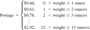
The rule in (1) is a function P consisting of 14 pieces (letters over 13 ounces are sent priority mail). A value P(w) is one of 14 constants; the constant changes depending on the weight w (in ounces) of the letter. ^* For example,

The domain of the function P is the union of the intervals:

EXAMPLE 1 Graph of a Piecewise-Defined Function

Graph the piecewise-defined function

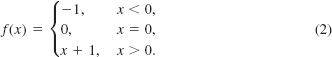
Solution Although the domain of f consists of all real numbers (–∞, ∞), each piece of the function is defined on a different part of this domain. We draw

 

the horizontal line y = – 1 for x < 0,

the point (0, 0) for x = 0, and

the line y = x + 1 for x > 0.

 

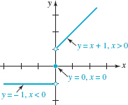
FIGURE 4.4.1 Graph of piecewise-defined function in Example 1

The graph is given in FIGURE 4.4.1.

The solid dot at the origin in FIGURE 4.4.1 indicates that the function in (2) is defined at x = 0 only by f(0) = 0; the open dots indicate that the formulas corresponding to x < 0 and to x > 0 do not define f at x = 0. Since we are making up a function, consider the definition

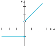
FIGURE 4.4.2 Graph of function g defined in (3)

The graph of g shown in FIGURE 4.4.2 is very similar to the graph of (2), but (2) and (3) are not the same function because f(0) = 0 but g(0) = – 1.

Greatest Integer Function We consider next a piecewise-defined function that is similar to the “postage stamp” function (1) in that both are examples of step functions; each function is constant on an interval and then jumps to another constant value on the next abutting interval. This new function, which has many notations, will be denoted here by , and is defined by the rule

The function f is called the greatest integer function because (4), translated into words, means that

f(x) is the greatest integer n that is less than or equal to x.

For example,

f(6) = 6 since 6 ≤ x = 6,	f(-1.5) = -2 since -2 ≤ x = -1.5,
f(0.4) = 0 since 0 ≤ x = 0.4,	f(7.6) = 7 since 7 ≤ x = 7.6,
f(π) =3 since 3 ≤ x = π,	f(-) = -2 since -2 ≤ x = -,

and so on. The domain of f is the set of real numbers and consists of the union of an infinite number of disjoint intervals, in other words, is a piecewise-defined function given by

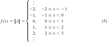
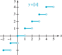
FIGURE 4.4.3 Greatest integer function

The range of f is the set of integers. A portion of the graph of f is given on the closed interval [–2, 5] in FIGURE 4.4.3.

In computer science the greatest integer function is known as the floor function and is denoted by See Problems 47, 48, and 53 in Exercises 4.4.

EXAMPLE 2 Shifted Graph

Graph

Solution The function is y = f(x - 2), where Thus the graph in FIGURE 4.4.3 is shifted horizontally 2 units to the right. Note in FIGURE 4.4.3 that if n is an integer, then But in FIGURE 4.4.4, for x = n, y = n - 2.

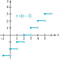
FIGURE 4.4.4 Shifted graph in Example 2

Continuous Functions The graph of a continuous function has no holes, finite gaps, or infinite breaks. While the formal definition of continuity of a function is an important topic of discussion in calculus, in this course it suffices to think in informal terms. A continuous function is often characterized by saying that its graph can be drawn “without lifting pencil from paper.” Parts (a)–(c) of FIGURE 4.4.5 illustrate functions that are not continuous, or discontinuous, at x = 2. The function

in Figure 4.4.5(a) has a hole in its graph (there is no point (2, f(2))); the function in Figure 4.4.5(b) has a finite gap or jump in its graph at x = 2; the function in Figure 4.4.5(c) has an infinite break in its graph x = 2. at The function f(x) = x³ – 3x + 2 is continuous; its graph given in Figure 4.4.5(d) has no holes, gaps, or infinite breaks.

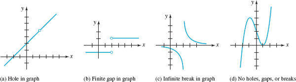
FIGURE 4.4.5 Discontinuous functions (a)-(c); continuous function (d)

You should be aware that constant functions, linear functions, and quadratic functions are continuous. Piecewise-defined functions can be continuous or discontinuous. The functions given in (2), (3), and (4) are discontinuous.

Absolute-Value Function The function y = |x| is called the absolute-value function. To obtain the graph, we graph its two pieces consisting of perpendicular half lines:

See Figure 4.4.6(a). Since y ≥ 0 for all x, another way of graphing (6) is simply to sketch the line y = x and then reflect in the x-axis that portion of the line that is below the x-axis. See Figure 4.4.6(b). The domain of (6) is the set of real numbers (– ∞, ∞), and as is seen in Figure 4.4.6(a), the absolute-value function is an even function, decreasing on the interval (– ∞, 0), increasing on the interval (0, ∞), and is continuous.

In some applications we are interested in the graph of the absolute value of an arbitrary function y = f(x), in other words, y = |f(x)|. Since |f(x)| is nonnegative for all numbers x in the domain of f, the graph of y = f(x) does not extend below the x-axis. Moreover, the definition of the absolute value of f(x),

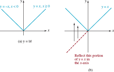
FIGURE 4.4.6 Absolute-value function (6)

shows that we must negate f(x) whenever f(x) is negative. There is no need to worry about solving the inequalities in (7); to obtain the graph of y = |f(x)|, we can proceed just as we did in Figure 4.4.6(b): Carefully draw the graph of y = f(x) and then reflect in the x-axis all portions of the graph that are below the x-axis.

EXAMPLE 3 Absolute Value of a Function

Graph y = | – 3x + 2 |

Solution We first draw the graph of the linear function f(x) = – 3x + 2. Note that since the slope is negative, f is decreasing and its graph crosses the x-axis at . We dash the graph for x > since that portion is below the x-axis. Finally, we reflect that portion upward in the x-axis to obtain the solid blue v-shaped graph in FIGURE 4.4.7. Since f(x) = x is a simple linear function, it is not surprising that the graph of the absolute value of any linear function f(x) = ax + b, a ≠ 0, will result in a graph similar to that of the absolute-value function shown in Figure 4.4.6(a).

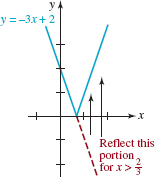
FIGURE 4.4.7 Graph of function in Example 3

EXAMPLE 4 Absolute Value of a Function

Graph y = | – x² + 2x + 3 |.

Solution As in Example 3 we begin by drawing the graph of the function f(x) = -x² + 2x + 3 by finding its intercepts (– 1, 0), (3, 0), (0, 3) and, since f is a quadratic function, its vertex (1, 4). Observe in Figure 4.4.8(a) that y < 0 for x < – 1 and for x > 3. These two portions of the graph of f are reflected in the x-axis to obtain the graph of y = | – x² + 2x + 3 | given in Figure 4.4.8(b).

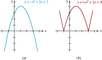
FIGURE 4.4.8 Graph of function in Example 4

4.4 Exercises Answers to selected odd-numbered problems begin on page ANS-9.

In Problems 1-4, find the indicated values of the given piecewise-defined function f.

1.

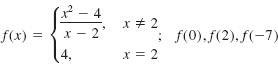
2.

3.

4.

5. If the piecewise-defined function f is defined by

find each of the following values.

(a)

(b)

(c)

(d)

(e) f(5, 72)

(f) f(π)

6. What is the y-intercept of the graph of the function f in Problem 5?

7. Determine the values of x for which the piecewise-defined function

(a) 7

(b) 0

(c) – 1

(d) – 2

(e) 1

(f) – 7

8. Determine the values of x for which the piecewise-defined function

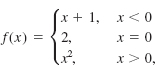
is equal to the given number.

(a) 1

(b) 0

(c) 4

(d)

(e) 2

(f) – 4

In Problems 9–34, sketch the graph of the given piecewise-defined function. Find any x-and y-intercepts of the graph. Give any numbers at which the function is discontinuous.

9.

10.

11.

12.

13. y = [|x + 2|]

14. y = 2 + [|x|]

15. y = – [|x|]

16. y = [| – x|]

17. y = |x + 3|

18. y = – |x – 4|

19. y = 2 – |x|

20. y = – 1 – |x|

21. y = – 2 + |x + 1 |

22.

23.

24.

25.

26.

27.

28.

29.

30.

31.

32.

33.

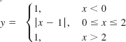
34.

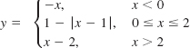
35. Without graphing, give the range of the function

36. Compare the graphs of y = 2[|x|] and y = [|2x|]

In Problems 37–40, find a piecewise-defined formula for the function f whose graph is given. Assume that the domain of f is (–∞, ∞)

37.

FIGURE 4.4.9 Graph for Problem 37

38.

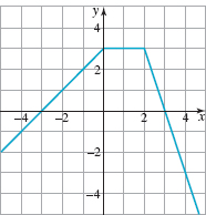
FIGURE 4.4.10 Graph for Problem 38

39.

FIGURE 4.4.11 Graph for Problem 39

40.

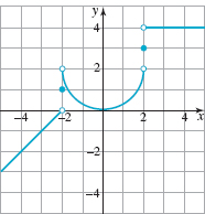
FIGURE 4.4.12 Graph for Problem 40

In Problems 41 and 42, sketch the graph of y = | f(x) |.

41. f is the function whose graph is given in FIGURE 4.4.9.

42. f is the function whose graph is given in FIGURE 4.4.10.

In Problems 43 and 44, use the definition of absolute value and express the given function f as a piecewise-defined function.

43.

44.

In Problems 45 and 46, find the value of the constant k such that the given piecewisedefined function f is continuous at x = 2 That is, the graph of f has no holes, gaps, or breaks in its graph at x = 2.

45.

46.

47. The ceiling function is defined to be the least integer n that is greater than or equal to x. Fill in the blanks

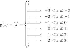
48. Graph the ceiling function defined in Problem 47.

For Discussion

In Problems 49-52, describe in words how the graphs of the given functions differ. [Hint: Factor and cancel.]

49.

50.

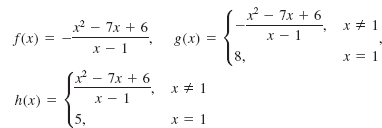
51.

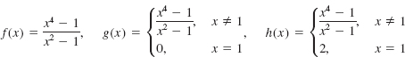
52.

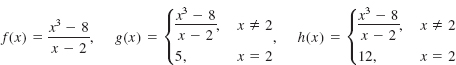
53. Using the notion of a reflection of a graph in an axis, express the ceiling function defined in Problem 47, in terms of the floor function (see page 187).

54. Discuss how to graph the function y = |x| + |x – 3|.

4.5 EBB Combining Functions

Introduction Two functions f and g can be combined in several ways to create new functions. In this section we examine two such ways in which functions can be combined: through arithmetic operations, and through the operation of function composition.

Arithmetic Combinations Two functions can be combined through the familiar four arithmetic operations of addition, subtraction, multiplication, and division.

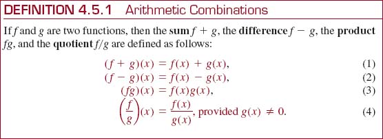
EXAMPLE 1 Sum, Difference, Product, and Quotient

Consider the functions f(x) = x² + 4x and g(x) = x² – 9. From (1)–(4) of Definition 4.5.1 we can produce four new functions:

and

Domain of an Arithmetic Combination When combining two functions arithmetically it is necessary that both f and g be defined at a same number x. Hence the domain of the functions f + g, f – g, and fg is the set of real numbers that are common to both domains; that is, the domain is the intersection of the domain off with the domain of g. In the case of the quotientf/g, the domain is also the intersection of the two domains, but we must also exclude any values of x for which the denominator g(x) is zero. In Example 1 the domain of f and the domain of g is the set of real numbers (– ∞, ∞), and so the domain of f + g, f – g, andfgis also (– ∞, ∞). However, since g(–3) = 0 and g(3) = 0, the domain of the quotient (f/g)(x) is (– ∞, ∞) with x = 3 and x = –3 excluded, in other words, (–∞, –3) ∪ (–3, 3) ∪ (3, ∞).In summary, if the domain of f is the set X_x and the domain of g is the set X₂, then

the domain of f + g, f – g, and fg is the intersection X₁ ∩ X₂, and

the domain of f/g is the set {x | x ε X₁ ∩ X₂, g(x) ≠ 0}.

EXAMPLE 2 Domain of f + g

By solving the inequality 1 – x ≥ 0, it is seen that the domain of is the interval (–∞, 1]. Similarly, the domain of the function is the interval [– 2, ∞). Hence, the domain of the sum

is the intersection (-∞, 1] ∩ [-2, ∞).You should verify this result by sketching these intervals on the number line and show that this intersection, or the set of numbers common to both domains, is the closed interval [-2, 1].

Composition of Functions Another method of combining functions f and g is called function composition. To illustrate the idea, let's suppose that for a given x in the domain of g the function value g(x) is a number in the domain of the function f. This means we are able to evaluate f at g(x), in other words, f(g(x)). For example, suppose f(x) = x² and g(x) = x + 2. Then for x = 1, g(l) = 3, and since 3 is the domain of f, we can write f(g(1)) = f(3) = 3² = 9. Indeed, for these two particular functions it turns out that we can evaluate f at any function value g(x), that is,

The resulting function, called the composition of f and g, is defined next.

When computing a composition such as (f g)(x) = f(g(x)) be sure to substitute g(x) for every x that appears in f(x). See part (a) of the next example.

EXAMPLE 3 Two Compositions

If f(x) = x² + 3x – 1 and g(x) = 2x² + 1, find (a) (f g)(x) and (b) (g f)(x).

Solution (a) For emphasis we replace x by the set of parentheses ( ) and write f in the form

Thus to evaluate (f g)(x) we fill each set of parentheses with g(x). We find

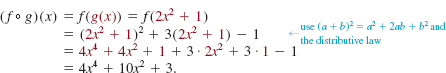
(b) In this case write g in the form

Then

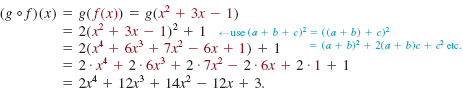
Parts (a) and (b) of Example 3 illustrate that function composition is not commutative. That is, in general

The next example shows that a function can be composed with itself.

EXAMPLE 4 f Composed with f

If f(x) = 5x – 1, then the composition

EXAMPLE 5 Writing a Function as a Composition

Express as the composition of two functions f and g.

Solution If we define f and g as and then

There are other solutions to Example 5. For instance, if the functions f and g are defined by and g(x) = x³, then observe

Domain of a Composition As stated in the introductory example to this discussion, to evaluate the composition (f g)(x) = f(g(x)) the number g(x) must be in the domain of f. For example, the domain and the domain of g(x) = x – 2 is the set of real numbers (– ∞, ∞). Observe we cannot evaluate f(g(1)) because g(1) = – 1 and – 1 is not in the domain off. In order to substitute g(x) into f(x), g(x) must satisfy the inequality that defines the domain off, namely, g(x) ≥ 0. This last inequality is the same as x – 2 ≥ 0 or x ≥ 2. The domain of the composition which is only a portion of the original domain (– ∞, ∞) of g. In general:

The domain of the composition f g consists of the numbers x in the domain of g such that the function values g(x) are in the domain of f.

EXAMPLE 6 Domain of a Composition

Consider the function From the requirement that x – 3 ≥ Owe see that whatever number x is substituted into f must satisfy x ≥ 3. Now suppose g(x) = x² + 2 and we want to evaluate f(g(x)). Although the domain of g is the set of all real numbers, in order to substitute g(x) into f(x) we require that x be a number in that domain so that g(x) ≥ 3. From FIGURE 4.5.1 we see that the last inequality is satisfied whenever x ≤ –1 or x ≥ 1.

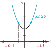
FIGURE 4.5.1 Domain of (f g)(x) in Example 6

In other words, the domain of the composition

In certain applications a quantity y is given as a function of a variable x, which in turn is a function of another variable t. By means of function composition we can express y as a function of t. The next example illustrates the idea; the symbol V plays the part of y and r plays the part of x.

EXAMPLE 7 Inflating a Balloon

A weather balloon is being inflated with a gas. If the radius of the balloon is increasing at a rate of 5 cm/s, express the volume of the balloon as a function of time t in seconds.

Solution Let's assume that as the balloon is inflated, its shape is that of a sphere. If r denotes the radius of the balloon, then r(t) = 5t. Since the volume of a sphere is , the composition is (V r)(t) = V(r(t)) = V(5t) or

Weather balloon

Transformations The rigid and nonrigid transformations that were considered in Section 4.2 are examples of the operations on functions discussed in this section. For c > 0 a constant, the rigid transformations defined by y = f(x) + c and y = f(x) – c are the sum and difference, respectively, of the function f(x) and the constant function g(x) = c. The nonrigid transformation y = cf(x) is the product of f(x) and the constant function g(x) = c. The rigid transformations defined by y = f(x + c) and y = f(x – c) are compositions of f(x) with the linear functions g(x) = x + c and g(x) = x – c, respectively.

FIGURE 4.5.2 Secant line through two points on a graph

Difference Quotient Suppose points P and Q are two distinct points on the graph of y = f(x) with coordinates (x, f(x)) and (x + h, f(x + h)), respectively. Then as shown in FIGURE 4.5.2, the slope of the secant line through P and Q is

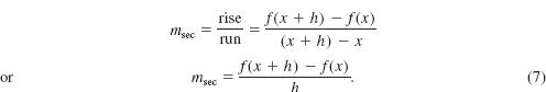
The expression in (7) is called a difference quotient and is very important in the study of calculus. The symbol h is just a real number and as seen in FIGURE 4.5.2 represents an increment or a change in x. The computation of (7) is essentially a three-step process and these steps involve only precalculus mathematics: algebra and trigonometry. Getting over the hurdles of algebraic or trigonometric manipulations in these steps is your primary goal. If you are preparing for calculus, we recommend that you be able to carry out the calculation of (7) for functions involving

positive integer powers of x such as xⁿ for n = 1, 2, and 3,

division of functions such as

radicals such as

See Problems 47–60 in Exercises 4.5.

EXAMPLE 8 Difference Quotient

(a) Compute the difference quotient (7) for the function y = x² + 2.

(b) Find the slope of the secant line through the points (2, f (2)) and (2.5, f (2.5)).

Solution (a) The initial step is the computation of f (x + h). For the given function we write f( ) = ( )² + 2. The idea is to substitute x + h into the parentheses and carry out the required algebra:

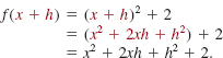
The second step, the computation of the differencef (x + h) – f(x), is the most important step and should be simplified as much as possible. In many of the problems that you will be required to do in calculus you will be able to factor h from the difference f (x + h) – f(x):

The computation of the difference quotient is now straightforward.

We use the results from the preceding step:

Thus the slope m_sec of the secant line is

(b) For the given points we identify x = 2 and the change in x as h = 2.5 – 2 = 0.5. Therefore the slope of the secant line that passes through (2, f(2)) and (2.5, f(2.5)) is given by m_sec = 2(2) 1 0.5 or m_sec = 4.5.

4.5 Exercises Answers to selected odd-numbered problems begin on page ANS-10.

In Problems 1-8, find the functions f + g, f – g, fg and f/g and give their domains.

1.

2.

3.

4.

5.

6.

7.

8.

9. Fill in the table.

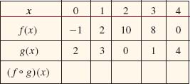
10. Fill in the table where g is an odd function.

In Problems 11–14, find the functions f g and g f and give their domains.

11.

12.

13.

14.

In Problems 15–20, find the functions f g and g f

15.

16.

17.

18.

19.

20.

In Problems 21–24, find f f and f (1/f)

21.

22.

23.

24.

In Problems 25 and 26, find (f g h)(x) f(g(h(x))).

25.

26.

27. For the functions

28. For the functions

In Problems 29 and 30, find (f f f)(x) = f(f(f(x))).

29. f(x) = 2x – 5

30. f(x) = x² – 1

In Problems 31–34, find functions f and g such that F(x) = f g.

31.

32.

33.

34.

In Problems 35 and 36, sketch the graphs of the compositions f g and g f.

35.

36.

37. Consider the function y = f(x) + g(x), where f(x) = x and g(x) = –[x]. Fill the blanks and then sketch the graph of the sum f + g over the indicated intervals.

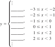
38. Consider the function y = f(x) + g(x), where f(x) = |x| and g(x) = [x] Proceed as in Problem 37 and then sketch the graph of the sum f + g

In Problems 39 and 40, sketch the graph of the sum f + g

39.

40.

In Problems 41 and 42, sketch the graph of the product fg.

41.

42.

In Problems 43 and 44, sketch the graph of the reciprocal 1/f

43. f(x) = |x|

44. f(x) = x – 3

In Problems 45 and 46, (a) find the points of intersection of the graphs of the given functions

(b) Find the vertical distance d between the graphs on the interval I determined by the x-coordinates of their points of intersection.

(c) Use the concept of a vertex of a parabola to find the maximum value of d on the interval I.

FIGURE 4.5.3 Graph for Problem 45

FIGURE 4.5.4 Graph for Problem 46

In Problems 47–58, (a) compute the difference quotient for the given function.

(b) Find the slope of the secant line through the two points (3, f(3)), (3.1, f(3.1))

47. f(x) = –4x²

48. f(x) = x² – x

49. f(x) = 3x² – x + 7

50. f(x) = 2x² + x – 1

51. f(x) = x³ + 5x – 4

52. f(x) = 2x³ + x²

53.

54.

55.

56.

57.

58.

In Problems 59 and 60, compute the difference quotient for the given function. Use appropriate algebra in order to cancel the h in the denominator.

59.

60.

FIGURE 4.5.5 Bird-watcher in Problem 61

Miscellaneous Applications

61. For the Birds A bird-watcher sights a bird 100 ft due east of her position. If the bird is flying due south at a rate of 500 ft/min, express the distance d from the bird-watcher to the bird as a function of time t. Find the distance 5 minutes after the sighting. See FIGURE 4.5.5.

62. Bacteria A certain bacteria when cultured grows in a circular shape. The radius of the circle, measured in centimeters, is given by the mathematical model

where time t is measured in hours.

(a) Express the area covered by the bacteria as a function of time t.

(b) Express the circumference of the area covered as a function of time t.

For Discussion

63. Suppose f(x) = x² + 1 and Discuss: Why is the domain of

64. Suppose Discuss: Why is the domain of

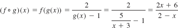not

65. Find the error in the following reasoning: If f(x) = 1/(x – 2) and then and so

66. Suppose and What is the domain of the function

67. Suppose and h(x) = –x. Discuss: Without actually graphing, how are the graphs of f g, g f, f h and h f related to the graph of f

68. The domain of each piecewise-defined function, is (–∞, ∞) Discuss how to find f + g, f – g, and fg Carry out your ideas.

69. Discuss how the graph of is related to the graph of y = f(x) Illustrate your ideas using f(x) = x² – 6x + 5.

70. Discuss:

(a) Is the sum of two even functions f and g even?

(b) Is the sum of two odd functions f and g odd?

(c) Is the product of an even function f with an odd function g even, odd, or neither?

(d) Is the product of an odd function f with an odd function g even, odd, or neither?

71. The product fg of two linear functions with real coefficients, f(x) = ax + b and g(x) = cx + d is a quadratic function. Discuss: Why must the graph of this quadratic function have at least one x-intercept?

72. Make up two different functions f and g so that the domain of F(x) = f g is [–2, 0) ∪ (0, 2].

4.6 Inverse Functions

Introduction Recall that a function f is a rule of correspondence that assigns to each value x in its domain X, a single or unique value y in its range. This rule does not preclude having the same number y associated with several different values of x. For example, for f(x) = x² + 1, the value y = 5 occurs at either x = –2 or x = 2 On the other hand, for the function g(x) = x³ the value y = 64 occurs only at x = 4. Indeed, for every value y in the range of the function g(x) = x³ there corresponds only one value of x in its domain. Functions of this last kind are given a special name.

Horizontal Line Test Interpreted geometrically, this means that a horizontal line (y = constant) can intersect the graph of a one-to-one function in at most one point. Furthermore, if every horizontal line that intersects the graph of a function does so in at most one point, then the function is necessarily one-to-one. A function is not one-to-one if some horizontal line intersects its graph more than once.

EXAMPLE 1 Horizontal Line Test

The graphs of the functions f(x) = x² + 1 and g(x) = x³, and a horizontal line y = c intersecting the graphs of f and g, are shown in FIGURE 4.6.1. Figure 4.6.1(a) indicates that there are two numbers x₁ and x₂ in the domain of f for which f(x₁) = f(x₂) = c. Inspection of Figure 4.6.1(b) shows that for every horizontal line y = c intersecting the graph, there is only one number x₁ in the domain of g such that g(x_x) = c. Hence the function f is not one-to-one, whereas the function g is one-to-one.

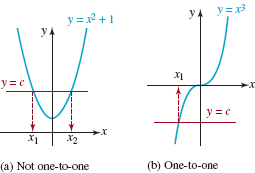
FIGURE 4.6.1 Two types of functions

A one-to-one function can be defined in several different ways. Based on the preceding discussion, the following statement should make sense.

Stated in a negative way, (1) indicates that a functionf is not one-to-one if different numbers x₁ and x₂ (that is, x₁ ≠ x₂) can be found in the domain of f such that f(x₁) = f(x₂). You will see this formulation of the one-to-one concept when we solve certain kinds of equations in Chapter 006.

You should consider (1) as a way of determining whether a function f is one-to-one without the benefit of a graph.

EXAMPLE 2 Checking for One-to-One

(a) Consider the function f(x) = x⁴ – 8x + 6. Observe that f(0) = f(2) = 6 but since 0 ≠ 2 we can conclude that f is not one-to-one.

(b) Consider the function and let x₁ and x₂ be numbers in the domain of f. If we assume f(x₁) = f(x₂), that is, then by taking the reciprocal of both sides we see

From (1) we conclude that f is one-to-one.

FIGURE 4.6.2 Functions f and f^-1

Inverse of a One-to-One Function Suppose f is a one-to-one function with domain X and range Y. Since every number y in Y corresponds to precisely one number x in X, the function f must actually determine a “reverse” function f^–1 whose domain is Y and range is X. As shown in FIGURE 4.6.2, f and f^–1 must satisfy

The equations in (2) are actually the compositions of the functions f and f^–1:

The function f^–1 is called the inverse of f or the inverse function for f. Following convention that each domain element be denoted by the symbol x, the first equation in (3) is rewritten as f(f^–1(x)) = x. We summarize the two results given in (3).

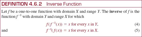
Of course, if a function f is not one-to-one, then it has no inverse function.

Properties Before we actually examine methods for finding the inverse of a one-to-one function f, let's list some important properties about f and its inverse f ^-1.

First Method for Finding f^–1 We will consider two ways of finding the inverse of a one-to-one function f. Both methods require that you solve an equation; the first method begins with (4).

EXAMPLE 3 Inverse of a Function

(a) Find the inverse of

(b) Find the domain and range of f^–1. Find the range off.

Solution (a) We proved in part (b) of Example 2 thatf is one-to-one. To find the inverse of f using (4), we must substitute the symbol f^–1(x) wherever x appears in f and then set the expression f (f ^–1(x)) equal to x:

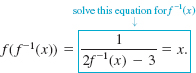
By taking the reciprocal of both sides of the equation in the blue outline box we get

Dividing both sides of the last equation by 2 yields the inverse of f:

(b) Inspection of f reveals that its domain is the set of real numbers except , that is, Moreover, from the inverse just found we see that the domain of f^–1 is . Because range of f^–1 = domain of f we then know that the range of f^–1 is . From domain of f^–1 = range of f we have also discovered that the range of f is

Second Method for Finding f^–1 The inverse of a function f can be found in a different manner. If f^-1 is the inverse of f, then x = f^–1(y). Thus we need only do the following two things:

Solve y = f(x) for the symbol x in terms of y (if possible). This gives x = f^-1(y).

Relabel the variable x as y and the variable y as x. This gives y = f^-1(x).

EXAMPLE 4 Inverse of a Function

Find the inverse of f(x) = x³.

Solution In Example 1 we saw that this function was one-to-one. To begin, we rewrite the function as y = x³ Solving for x then gives y = x^1/3. Next we relabel variables to obtain y = x^1/3. Thus f^–1(x) = x^1/3 or equivalently

Finding the inverse of a one-to-one function y = f(x) is sometimes difficult and at times impossible. For example, it can be shown that the function f(x) = x³ + x + 3 is one-to-one and so has an inverse f^–1, but solving the equation y = x³ + x + 3 for x is difficult for everyone (including your instructor). Nevertheless, since f only involves positive integer powers of x, its domain is (–∞, ∞). If you investigate. f graphically you are led to the fact that the range of f is also (–∞, ∞). Consequently the domain and range of f^–1 are (–∞, ∞). Even though we don't know f^–1 explicitly it makes complete sense to talk about the values such as f^–1(3) and f^–1(5). In the case of f^–1(3) note that f(0) = 3. This means that f^–1(3) = O. Can you figure out the value of f^–1(5)?

Graphs off f and f^–1 Suppose that (a, b) represents any point on the graph of a one-to-one function f. Then f(a) = b and

implies that (b, a) is a point on the graph of f^–1. As shown in Figure 4.6.3(a), the points (a, b) and (b, a) are reflections of each other in line y = x. This means that the line y = x is the perpendicular bisector of the line segment from (a, b) to (b, a). Because each point on one graph is the reflection of a corresponding point on the other graph, we see in Figure 4.6.3(b) that the graphs of f^–1 and f are reflections of each other in the line y = x. We also say that the graphs of f^–1 and f are symmetric with respect to the line y = x.

FIGURE 4.6.3 Graphs of f and f^–1 are reflections in the line y = x

EXAMPLE 5 Graphs of f and f^–1

In Example 4 we saw that the inverse of y = x³ is y = x^1/3. In Figure 4.6.4(a) and Figure 4.6.4(b) we show the graphs of these functions; in Figure 4.6.4(c) the graphs are superimposed on the same coordinate system to illustrate that the graphs are reflections of each other in the line y = x.

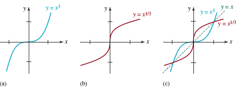
FIGURE 4.6.4 Graphs of f and f^–1 in Example 5

Every linear function f(x) = ax + b, a ≠ 0, is one-to-one.

EXAMPLE 6 Inverse of a Function

Find the inverse of the linear function f (x) = 5x – 7.

Solution Since the graph of y = 5x – 7 is a nonhorizontal line, it follows from the horizontal line test that f is a one-to-one function. To find f^–1 solve y = 5x – 7 for x:

Relabeling the two variables in the last equation gives Therefore The graphs of f and f^–1 are compared in FIGURE 4.6.5.

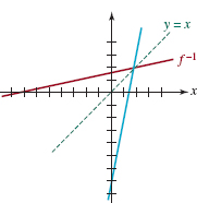
FIGURE 4.6.5 Graphs of f and f^–1 in Example 6

Every quadratic function f(x) = ax² + bx + c, a ≠ 0, is not one-to-one.

Restricted Domains For a function f that is not one-to-one, it may be possible to restrict its domain in such a manner so that the new function consisting of f defined on this restricted domain is one-to-one and so has an inverse. In most cases we want to restrict the domain so that the new function retains its original range. The next example illustrates this concept.

EXAMPLE 7 Restricted Domain

In Example 1 we showed graphically that the quadratic function f(x) = x² + 1 is not one-to-one. The domain of f is (–∞, ∞), and as seen in Figure 4.6.6(a), the range of f is [1, ∞). Now by defining f(x) = x² + 1 only on the interval [0, ∞), we see two things in Figure 4.6.6(b): The range of f is preserved and f(x) = x² + 1 confined to the domain [0, ∞) passes the horizontal line test, in other words, is one-to-one. The inverse of this new one-to-one function is obtained in the usual manner. Solving y = x² + 1 implies

The appropriate algebraic sign in the last equation is determined from the fact that the domain and range of f^–1 are [1, ∞) and [0, ∞), respectively. This forces us to choose as the inverse of f. See Figure 4.6.6(c).

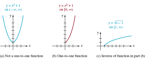
FIGURE 4.6.6 Inverse function in Example 7

4.6 Exercises Exercises Answers to selected odd-numbered problems begin on page ANS-10.

In Problems 1-6, the graph of a function f is given. Use the horizontal line test to determine whether f is one-to-one.

1.

FIGURE 4.6.7 Graph for Problem 1

2.

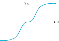
FIGURE 4.6.8 Graph for Problem 2

3.

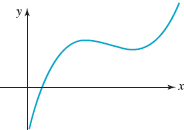
FIGURE 4.6.9 Graph for Problem 3

4.

FIGURE 4.6.10 Graph for Problem 4

5.

FIGURE 4.6.11 Graph for Problem 5

6.

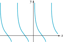
FIGURE 4.6.12 Graph for Problem 6

In Problems 7-10, sketch the graph of the given piecewise-defined function f to determine whether it is one-to-one.

7.

8.

9.

10.

In Problems 11-14, proceed as in Example 2(a) to show that the given function fis not one-to-one.

11.

12.

13.

14.

In Problems 15-18, proceed as in Example 2(b) to show that the given function fis one-to-one.

15.

16.

17.

18.

In Problems 19 and 20, the given function f is one-to-one. Without finding f ¹ find its domain and range.

19.

20.

In Problems 21 and 22, the given function f is one-to-one. The domain and range of f is indicated. Find f²¹ and give its domain and range.

21.

22.

In Problems 23-28, the given function f is one-to-one. Find f Sketch the graph of f and f^–1 on the same coordinate axes.

23.

24.

25.

26.

27.

28.

In Problems 29-32, the given functionf is one-to-one. Findf ¹. Proceed as in Example 3(b) and find the domain and range of f^–1. Then find the range off.

29.

30.

31.

32.

In Problems 33-36, the given function f is one-to-one. Without finding f f find the point on the graph of f^–1 corresponding to the indicated value of x in the domain of f.

33.

34.

35.

36.

In Problems 37 and 38, sketch the graph of f ¹ from the graph of f.

37.

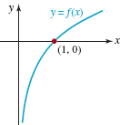
FIGURE 4.6.13 Graph for Problem 37

38.

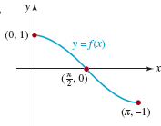
FIGURE 4.6.14 Graph for Problem 38

In Problems 39 and 40, sketch the graph of f from the graph of f^–1.

39.

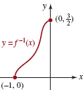
FIGURE 4.6.15 Graph for Problem 39

40.

FIGURE 4.6.16 Graph for Problem 40

In Problems 41-44, the function f is not one-to-one on the given domain but is one-to-one on the restricted domain (the second interval). Find the inverse of the one-to-one function and give its domain. Sketch the graph of f on the restricted domain and the graph of f²¹ on the same coordinate axes.

41.

42.

43.

44.

In Problems 45 and 46, verify that f (f^-1(x)) = x and f^–1(f(x)) = x.

45.

46.

For Discussion

47. Suppose f is a continuous function that is increasing (or decreasing) for all x in its domain. Explain why f is necessarily one-to-one.

48. Explain why the graph of a one-to-one function f can have at most one x-intercept.

49. The function f(x) = |2x – 41 is not one-to-one. How should the domain of f be restricted so that the new function has an inverse? Find f^-1 and give its domain and range. Sketch the graph of f on the restricted domain and the graph of f^-1 on the same coordinate axes.

50. The equation defines a one-to-one function y = f(x).Find f^–1(x).

51. What property do the one-to-one functions y = f(x) shown in FIGURE 4.6.17 have in common? Find two more explicit functions with this same property. Be very clear about what this property has to do with f^–1.

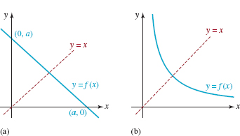
FIGURE 4.6.17 Graphs for Problem 51

4.7 Building a Function from Words

Introduction In subsequent courses in mathematics there are instances when you will be expected to translate the words that describe a problem into mathematical symbols and then set up or construct either an equation or a function.

In this section we focus on problems that involve functions. We begin with a verbal description about the product of two numbers.

EXAMPLE 1 Product of Two Numbers

The sum of two nonnegative numbers is 15. Express the product of one and the square of the other as a function of one of the numbers.

Solution We first represent the two numbers by the symbols x and y and recall that “nonnegative” means that x ≥ 0 and y ≥ 0. The first sentence then says that x + y = 15; this is not the function we are seeking. The second sentence describes the function we want; it is called “the product.” Let's denote “the product” by the symbol P. Now P is the product of one of the numbers, say, x and the square of the other, that is, y²:

No, we are not finished because P is supposed to be a “function of one of the numbers.” We now use the fact that the numbers x and y are related by x + y = 15. From this last equation we substitute y = 15 – x into (1) to obtain the desired result:

Here is a symbolic summary of the analysis of the problem given in Example 1:

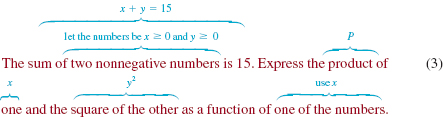
Notice that the second sentence is vague about which number is squared. This means that it really doesn't matter; (1) could also be written as P = yx². Also, we could have used x = 15 – y in (1) to arrive at P(y) = (15 – y)y². In a course such as calculus it would not have mattered whether we worked with P(x) or with P(y) because by finding one of the numbers we automatically find the other from the equation x + y = 15. This last equation is commonly called a constraint. A constraint not only defines the relationship between the variables x and y but often puts a limitation on how x and y can vary. As we see in the next example, the constraint helps in determining the domain of the function that you have just constructed.

EXAMPLE 2 Example 1 Continued

What is the domain of the function P(x) in (2)?

Solution Taken out of the context of the statement of the problem in Example 1, one would have to conclude from the discussion on page 157 of Section 4.1 that the domain of the cubic polynomial function

is the set of real numbers (–∞, ∞). But in the context of the original problem, the numbers were to be nonnegative. From the requirement that x ≥ 0 and y = 15 – x ≥ 0 we get x ≥ 0 and x ≤ 15, which means that x must satisfy the simultaneous inequality 0 ≤ x ≤ 15. Using interval notation, the domain of the product function P in (2) is the closed interval [0, 15].

Another way of looking at the conclusion of Example 2 is this: The constraint x + y = 15 dictates that y = 15 – x. Thus if x were allowed to be larger than 15 (say, x = 17.5), then y = 15 – x would be a negative number that contradicts the initial assumption that y ≥ 0.

Invariably whenever word problems are discussed in a mathematics class, students often react with groans, ambivalence, and dismay. While not guaranteeing anything, the following suggestions might help you to get through the problems in Exercises 4.7. These problems are especially important if your future plans include taking a course in calculus.

EXAMPLE 3 Area of a Rectangle

A rectangle has two vertices on the x-axis and two vertices on the semicircle whose equation is See Figure 4.7.1(a). Express the area of the rectangle as a function of x.

FIGURE 4.7.1 Rectangle in Example 3

Solution If (x, y), x > 0, y > 0, denotes the vertex of the rectangle on the circle in the first quadrant, then as shown in Figure 4.7.1(b) the area A is length X width, or

The constraint in this problem is the equation of the semicircle. We use the constraint equation to eliminate y in (4) and obtain the area of the rectangle

Were we again to consider the function A(x) out of the context of the problem in Example 3, its domain would be [–5, 5]. Because we assumed that x > 0 we can take the domain of A(x) in (4) to be the open interval (0, 5).

EXAMPLE 4 Amount of Fencing

A rancher intends to mark off a rectangular plot of land that will have an area of 1000 m². The plot will be fenced and divided into two equal portions by an additional fence parallel to two sides. Express the amount of fencing used to enclose the plot of land as a function of the length of one side of the plot.

Solution A sketch of the land enclosed by the fence is a rectangle with a line drawn down its middle, similar to that given in FIGURE 4.7.2. As shown in the figure, let x > 0 be the length of the rectangular plot of land and let y > 0 denote its width. If the symbol F represents this amount, then the sum of the lengths of the five portions—two horizontal and three vertical—of the fence is

Since we want F to be a function of the length of one side of the plot of land we must eliminate either x or y from (6). Because the fenced-in land is to have an area of 1000 m², x and y are related by the constraint xy = 1000. From the last equation we get y = 1000/x, which can be used to eliminate y in (6). Thus, the amount of fence F as a function of x is F(x) = 2x 1 3(1000/x) or

FIGURE 4.7.2 Rectangular plot of land in Example 4

Since x represents a physical dimension that satisfies xy = 1000, we conclude that it is positive. But other than that, there is no restriction on x. Notice that if the positive number x is close to 0 then y = 1000/x is very large, whereas if x is taken to be a very large number, then y is close to 0. Thus the domain of F(x) is (0, ∞).

If a problem involves triangles, you should study the problem carefully and determine whether the Pythagorean theorem, similar triangles, or trigonometry is applicable (see Section 8.2).

EXAMPLE 5 Length of a Ladder

A 10-ft wall stands 5 ft from a building. A ladder, supported by the wall, touches a building as shown in FIGURE 4.7.3. Express the length of the ladder as a function of x shown in the figure.

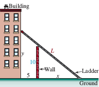
FIGURE 4.7.3 Ladder in Example 5

Solution Let L denote the length of the ladder. With x and y defined in FIGURE 4.7.3, we see that there are two right triangles; the larger triangle has three sides with lengths L, y, and x 1 5 and the smaller triangle has two sides of lengths x and 10. Now the ladder is the hypotenuse of the larger right triangle, so by the Pythagorean theorem,

The right triangles in FIGURE 4.7.3 are similar because they both contain a right angle and share the common acute angle the ladder makes with the ground. We then use the fact that the ratios of corresponding sides of similar triangles are equal. This enables us to write the constraint

Solving the last equation for y in terms of x gives y = 10(x + 5)/x, and so (8) becomes

Taking the square root gives us L as a function of x,

The domain of the function L(x) is (0, ∞).

EXAMPLE 6 Distance to a Point

Express the distance from a point (x, y) in the first quadrant on the circle x² + y² = 1 to the point (2, 4) as a function of x.

Solution Let d represent the distance from (x, y) to (2, 4). See FIGURE 4.7.4. Then from the distance formula, (2) of Section 3.1,

The constraint in this problem is the equation of the circle x² + y² = 1. From this we can immediately replace x² + y² in (9) by the number 1. Moreover, using the constraint to write allows us to eliminate y in (9). Thus the distance d as a function of x is

Because (x, y) is a point on the circle in the first quadrant the variable x can range from 0 to 1; that is, the domain of the function in (10) is the closed interval [0, 1].

FIGURE 4.7.4 Distance d in Example 6

NOTES FROM THE CLASSROOM

You should not get the impression that every problem that requires you to set up a function from a verbal description must have a constraint. In Problems 11–16 of Exercises 4.7 the required function can be set up using just one variable.

4.7 Exercises Answers to selected odd-numbered problems begin on page ANS-11.

In Problems 1-40, translate the words into an appropriate function. Give the domain of the function.

1. The product of two positive numbers is 50. Express their sum as a function of one of the numbers.

2. Express the sum of a nonzero number and its reciprocal as a function of the number.

3. The sum of two nonnegative numbers is 1. Express the sum of the square of one and twice the square of the other as a function of one of the numbers.

4. Let m and n be positive integers. The sum of two nonnegative numbers is S. Express the product of the mth power of one and the nth power of the other as a function of one of the numbers.

5. A rectangle has a perimeter of 200 in. Express the area of the rectangle as a function of the length of one of its sides.

6. A rectangle has an area of 400 in². Express the perimeter of the rectangle as a function of the length of one of its sides.

7. Express the area of the rectangle shaded in FIGURE 4.7.5 as a function of x.

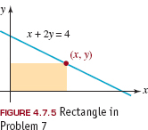
FIGURE 4.7.5 Rectangle in Problem 7

8. Express the length of the line segment containing the point (2, 4) shown in FIGURE 4.7.6 as a function of x.

FIGURE 4.7.6 Line segment in Problem 8

9. Express the distance from a point (x, y) on the graph of x + y = 1 to the point (2, 3) as a function of x.

10. Express the distance from a point (x, y) on the graph of y = 4 – x² to the point (0, 1) as a function of x.

11. Express the perimeter of a square as a function of its area A.

12. Express the area of a circle as a function of its diameter d.

13. Express the diameter of a circle as a function of its circumference C.

14. Express the volume of a cube as a function of the area A of its base.

15. Express the area of an equilateral triangle as a function of its height h.

16. Express the area of an equilateral triangle as a function of the length 5 of one of its sides.

17. A wire of length x is bent into the shape of a circle. Express the area of the circle as a function of x.

18. A wire of length L is cut x units from one end. One piece of the wire is bent into a square and the other piece is bent into a circle. Express the sum of the areas as a function of x.

19. A tree is planted 30 ft from the base of a street lamp that is 25 ft tall. Express the length of the tree's shadow as a function of its height. See FIGURE 4.7.7.

20. The frame of a kite consists of six pieces of lightweight plastic. The outer frame of the kite consists of four precut pieces; two pieces of length 2 ft and two pieces of length 3 ft. Express the area of the kite as a function of x, where 2x is the length of the horizontal crossbar piece shown in FIGURE 4.7.8.

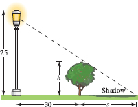
FIGURE 4.7.7 Tree in Problem 19

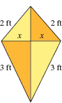
FIGURE 4.7.8 Kite in Problem 20

21. A company wants to construct an open rectangular box with a volume of 450 in³ so that the length of its base is 3 times its width. Express the surface area of the box as a function of the width.

22. A conical tank, with vertex down, has a radius of 5 ft and a height of 15 ft. Water is pumped into the tank. Express the volume of the water as a function of its depth. [Hint: The volume of a cone is Although the tank is a three-dimensional object, examine it in cross section as a two-dimensional triangle. See FIGURE 4.7.9.]

FIGURE 4.7.9 Conical tank in Problem 22

23. Car A passes point O heading east at a constant rate of 40 mi/h; car B passes the same point 1 hour later heading north at a constant rate of 60 mi/h. Express the distance between the cars as a function of time t, where t is measured starting when car B passes point O. See FIGURE 4.7.10.

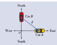
FIGURE 4.7.10 Cars in Problem 23

24. At time t = 0 (measured in hours), two airliners with a vertical separation of 1 mile, pass each other going in opposite directions. If the planes are flying horizontally at rates of 500 mi/h and 550 mi/h, express the horizontal distance between them as a function of t. [Hint: Distance = rate X time.]

25. The swimming pool shown in FIGURE 4.7.11 is 3 ft deep at the shallow end, 8 ft deep at the deepest end, 40 ft long, 30 ft wide, and the bottom is an inclined plane. Water is pumped into the pool. Express the volume of the water in the pool as a function of height h of the water above the deep end. [Hint: The volume will be a piecewise-defined function with domain defined by 0 ≤ h ≤ 8.]

26. U.S. Postal Service regulations for parcel post stipulate that the length plus girth (the perimeter of one end) of a package must not exceed 108 inches. Express the volume of the package as a function of the width x shown in FIGURE 4.7.12.[Hint: Assume that the length plus girth equals 108.]

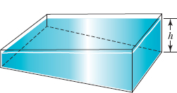
FIGURE 4.7.11 Swimming pool in Problem 25

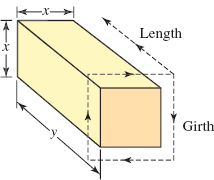
FIGURE 4.7.12 Package in Problem 26

27. Consider all rectangles that have the same perimeter p. (Here p represents a constant.) Express the area of such a rectangle as a function of the length of one side.

28. The length of a rectangle is x, its height is y, and its perimeter is 20 inches. Express the length of the diagonal of the rectangle as a function of the length x.

29. A rectangular plot of land will be fenced into three equal portions by two dividing fences parallel to two sides. If the area to be enclosed is 4000 m², express the amount of fence needed as a function of the length of the plot of land.

30. A rectangular plot of land will be fenced into three equal portions by two dividing fences parallel to two sides. If the total fence to be used is 8000 m, express the area of the fenced land as a function.

31. A rancher wishes to build a rectangular corral with an area of 128,000 ft² with one side along a straight river. The fence along the river costs $1.50 per foot, whereas along the other three sides the fence costs $2.50 per foot. Express the cost of construction as a function of the length of fence along the river. [Hint: Along the river the cost of x ft of fence is 1.50x.]

32. Express the area of the colored triangular region shown in FIGURE 4.7.13 as a function of x.

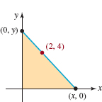
FIGURE 4.7.13 Triangular region in Problem 32

33. An open rectangular box is to be constructed with a square base and a volume of 32,000 cm³. Express the amount of material used in its construction as a function of x. See FIGURE 4.7.14.

FIGURE 4.7.14 Box in Problem 33

34. A closed rectangular box is to be constructed with a square base. The material for the top costs $2 per square foot, whereas the material for the remaining sides costs $1 per square foot. The total cost to construct each box is $36. Express the volume of the box as a function of the length of one side of the base.

35. A rain gutter with a rectangular cross section is made from a 1-ft X 20-ft piece of metal by bending up equal amounts from the 1-ft side. See FIGURE 4.7.15. Express the capacity of the gutter as a function of x. [Hint: Capcity = volume.]

FIGURE 4.7.15 Rain gutter in Problem 35

36. A juice can is to be made in the form of a right circular cylinder and have a volume of 32 in3. See Figure 4.7.16(a). Express the amount of material used in its construction as a function of the radius r of the circular cylinder. [Hint: Material 5 total surface area of can 5 area of top 1 area of bottom 1 area of lateral side. If the circular top and bottom covers are removed and the cylinder is cut straight up its side and flattened out, the result is the rectangle shown in Figure 4.7.16(c).]

37. A printed page will have 2-inch margins of white space on the sides and 1-inch margins of white space on the top and bottom. See FIGURE 4.7.17. The area of the printed portion is 32 in². Express the area of the page as a function of the height of the printed portion.

FIGURE 4.7.16 Juice can in Problem 36

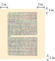
FIGURE 4.7.17 Printed page in Problem 37

38. Many medications are packaged in capsules as shown in the accompanying photo. Assume that a capsule is formed by adjoining two hemispheres to the ends of a right circular cylinder as shown in FIGURE 4.7.18. The total volume of the capsule is to be 0.007 in³. Express the amount of material used in its construction as a function of the radius r of each hemisphere. [Hint: The volume of a sphere is and its surface area is .]

Capsules

39. A 20-ft long water trough has ends in the form of isosceles triangles with sides that are 4 ft long. Express the volume of the trough as a function of the length x shown in FIGURE 4.7.19. [Hint: A right cylinder is not necessarily a circular cylinder where the top and bottom are circles. The top and bottom of a right cylinder are the same but could be a triangle, a pentagon, a trapezoid, and so on. The volume of a right cylinder is the area of the base X the height.]

FIGURE 4.7.18 Model of a capsule in Problem 38

FIGURE 4.7.19 Water trough in Problem 39

40. Some birds fly more slowly over water than over land. A bird flies at constant rates 6 km/h over water and 10 km/h over land. Use the information in FIGURE 4.7.20 to express the total flying time between the shore of one island and its nest on the shore of another island in terms of x. [Hint: Distance = rate X time.]

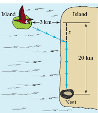
FIGURE 4.7.20 The bird in Problem 40

For Discussion

41. In Problem 19, what happens to the length of the tree's shadow as its height approaches 25 ft?

42. In an engineering text, the area of the octagon shown in FIGURE 4.7.21 is given as A = 3.31r². Show that this formula is actually an approximation to the area; that is, find the exact area A of the octagon as a function of r.

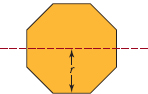
FIGURE 4.7.21 Octagon in Problem 42

4.8 Least Squares Line

Introduction When performing experiments, we often tabulate data in the form of ordered pairs (x₁, y₂), (x₂, y₂),…, (x_n, y_n), with each x_i distinct. Given the data, it is then often desirable to be able to extrapolate or predict y from x by finding a mathematical model—that is, a function that approximates or “fits” the data. In other words, we want a function f such that

Naturally, we do not want just any function but a function that fits the data as closely as possible. In the discussion that follows we shall confine our attention to the problem of finding a linear polynomial y = mx + b or a straight line that “best fits” the data (x₁, y₁),(x₂, y₂),…, (x_n, y_n). The procedure for finding this linear function is known as the method of least squares.

EXAMPLE 1 Fitting a Line to Data

Consider the data (1, 1), (2, 2), (3, 4), (4, 6), (5, 5) shown in Figure 4.8.1(a). Looking at Figure 4.8.1(b) and seeing that the line y = x + 1 passes through two of the data points, we might take this line as the one that best fits the data.

FIGURE 4.8.1 Data in (a); a line fitting data in (b)

Obviously we need something better than a visual guess to determine the linear function y = f(x) as in Example 1. We need a criterion that defines the concept of “best fit” or, as it is sometimes called, the “goodness of fit.”

If we try to match the data points with the line y = mx + b, then we wish to find m and b that satisfy the system of equations

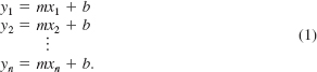
The system of equations (1) is an example of an overdetermined system; that is, a system in which the number of equations is greater than the number of unknowns. We do not expect such a system to have a solution unless, of course, the data points all lie on the same line.

Least Squares Line If the data points are (x₁, y₁), (x₂, y₂),…, (x_n, y_n), then one manner of determining how well the linear function f(x) = mx + b fits the data is to measure the vertical distances between the points and the graph of f:

We can think of each e_i as the error in approximating the data value y_i by the function value f(x_i). See FIGURE 4.8.2. Intuitively, the function f will fit the data well if the sum of all the e_i is a minimum. Actually, a more convenient approach to the problem is to find a linear function f so that the sum of the squares of all the e_i is a minimum. We shall define the solution of the system (1) to be those coefficients m and b that minimize the expression

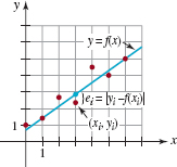
FIGURE 4.8.2 Error in approximating y_i by f(x_i)

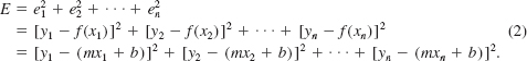
The expression E is called the sum of the square errors. The line y = mx + b that minimizes the sum of the square errors (2) is called the least squares line or the line of best fit for the data (x₁, y₁), (x₂, y₂),…, (x_n, y_n).

Summation Notation Before proceeding to find the least squares line it is convenient to introduce a shorthand notation for sums of numbers. Writing out sums such as (1) can become very tedious. Suppose a_k denotes a real number that depends on an integer k. The sum of n such real numbers a_k, a₁ + a₂ + a₃ +…+ aⁿ + a_n is denoted by the symbol that is,

Since ∑ is the capital Greek letter sigma, (3) is called summation notation or sigma notation. The integer k is called the index of summation and takes on consecutive integer values starting with k = 1 and ending with k = n. For example, the sum of the first 100 squared positive integers,

can be written compactly as

Written using sigma notation the sum of the square errors (2) can be written compactly as

The problem remains now, can one find a slope m and a y-coordinate b so that (4) is minimum? The answer is: Yes. Although we shall forego the details (which require calculus), the values of m and b that yield the minimum value of E are given by

EXAMPLE 2 Least Squares Line

Find the least squares line for the data in Example 1. Calculate the sum of the square errors E for this line and the line y = x + 1.

Solution From the data (1, 1), (2, 2), (3, 4), (4, 6), (5, 5) we identify x₁ = 1, x₂ = 2, x₃ = 3, x₄ = 4, x₅ = 5, y₁ = 1, y₂ = 3, y₃ = 4, y₄ = 6, and y₅ = 5. With these values and n = 5, we have

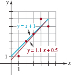
FIGURE 4.8.3 Least squares line (red) in Example 2

Substituting these values into the formulas in (5) yields m = 1.1 and b = 0.5. Thus, the least squares line is y = 1.1x + 0.5. By way of comparison, FIGURE 4.8.3 shows the data, the line y = x + 1 in blue and the least squares line y = 1.1x + 0.5 in red.

For the least squares line f(x) = 1.1x + 0.5 found in Example 2 the sum of the square errors (4) is

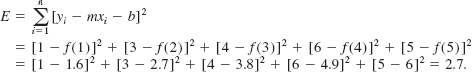
For the line y = x + 1 that we guessed in Example 1 that also passed through two of the data points, we find the sum of the square errors is E = 3.0.

In Section 9.6 we will examine another method for obtaining a least squares lines.

It is possible to generalize the least squares technique. For example, we might want to fit the given data to a quadratic polynomial f(x) = ax² + bx + c instead of a linear polynomial.

4.8 Exercises Answers to selected odd-numbered problems begin on page ANS-11.

In Problems 1–6, find the least squares line for the given data.

1. (2, 1), (3, 2), (4, 3), (5, 2)

2. (0, –1), (1, 3), (2, 5), (3, 7)

3. (1, 1), (2, 1.5), (3, 3), (4, 4.5), (5, 5)

4. (0, 0), (2, 1.5), (3, 3), (4, 4.5), (5, 5)

5. (0, 2), (1, 3), (2, 5), (3, 5), (4, 9), (5, 8), (6, 10)

6. (1, 2), (2, 2.5), (3, 1), (4, 1.5), (5, 2), (6, 3.2), (7, 5)

Miscellaneous Applications

7. In an experiment the correspondence given in the table was found between temperature T (in °C) and kinematic viscosity v (in Centistokes) of an oil with a certain additive. Find the least squares line v = mT + b. Use this line to estimate the viscosity of the oil at T = 140 and T = 160.

8. In an experiment the correspondence given in the table was found between temperature T (in °C) and electrical resistance R (in M). Find the least squares line R = mT + b. Use this line to estimate the resistance at T = 700.

Calculator/CAS Problems

9. (a) A set of data points can be approximated by a least squares polynomial of degree n. Learn the syntax for the CAS you have at hand, to obtain a least squares line (linear polynomial), a least squares quadratic, and a least squares cubic to fit the data

(b) Use a CAS to superimpose the plots of the data and the least squares line obtained in part (a) on the same coordinate axes. Repeat for the plots of the data and the least squares quadratic and then the data and the least squares cubic.

10. Use the U.S. census data (in millions) from the year 1900 through 2000

and a least squares line to predict the U.S. population in the year 2020.

CHAPTER 4 Exercises Review Exercises Answers to selected odd-numbered problems begin on page ANS-11.

A. True/False_____________________________________________

In Problems 1–22, answer true or false:

1. If (4, 0) is on the graph of f, then (1, 0) must be on the graph of y = f(x).____

2. The graph of a function can have only one y-intercept.____

3. If f is a function such that f(a) = f(b), then a = b._____

4. No nonzero function f can be symmetric with respect to the x-axis.____

5. The domain of f(x) = (x – 1)^1/3 is (–∞, ∞).____

6. If f(x) = x and then the domain of g/f is [–2, ∞).____

7. A function f is one-to-one if it never takes on the same value twice.____

8. The domain of the function y = is (–∞, 0].____

9. The graph of y = is a reflection of the graph of f(x) = in the y-axis.____

10. A point of intersection of the graphs of f and f^–1 must lie on the line y = x.____

11. The one-to-one function f(x) = 1/x has the property that f = f^–1._____

12. The function f(x) = 2x² + 16x – 2 decreases on the interval [–7, –5]._____

13. No even function defined on (– a, a), a > 0, can be one-to-one._____

14. All odd functions are one-to-one.______

15. If a function f is one-to-one, then _____

16. If f is an increasing function on an interval containing x₁ < x₂, then f (x₁) < f(x₂).____

17. The function f(x) = |x| – 1 is decreasing on the interval [0, ∞).____

18. For function composition, ____

19. If the y-intercept for the graph of a function f is (0, 1), then the y-intercept for the graph of y = 5 – 3f(x) is (0, 2).____

20. If f is a linear function, then f(x₁ + x₂) = f(x₁) + f(x₂).____

21. The function f(x) = x² + 2x + 1 is one-to-one on the restricted domain [–1, ∞). The range of f^–1 is also [–1,∞)._____

22. The function f(x) = x³ + 2x] + 5 is one-to-one. The point (8, 1) is on the graph of f^–1. _____

B. Fill in the Blanks

In Problems 1–20, fill in the blanks.

1. If then (, ___) is a point on the graph of f.

2. If and f(2) = 3, then A = _______.

3. The domain of the function is ____.

4. The range of the function f(x) = |x| – 10 is_____.

5. The zeros of the function are_____.

6. If the graph of f is symmetric with respect to the y-axis, f (–x) = ______.

7. If f is an odd function such that f (–2) = 2, then f(2) = ______.

8. The graph of a linear function for which f (–1) = 1 and f (1) = 5 has slope m = ______.

9. A linear function whose intercepts are (– 1, 0) and (0, 4) is f(x) = _____.

10. If the graph of y = |x – 2| is shifted 4 units to the left, then its equation is ________.

11. The x- and y-intercepts of the parabola f(x) = x² – 2x – 1 are ______.

12. The range of the function f(x) = –x² + 6x – 21 is _____.

13. The quadratic function f(x) = ax² + bx + c for which f(0) = 7 and whose only x-intercept is (–2, 0) is f(x) = ______.

14. If f(x) = x + 2 and g(x) = x² – 2x, then (f g)(–1) = _____.

15. The vertex of the graph of f(x) = x² is (0, 0). Therefore, the vertex of the graph of y = –5(x – 10)² + 2 is ____.

16. Given that is the inverse of a one-to-one function f. Without finding f, the domain of f is____and the range of f is_____.

17. The x-intercept of a one-to-one function f is (5, 0) and so the y-intercept of f^–1 is______.

18. The inverse of is f^–1 =_____.

19. For =_____.

20. If f is a one-to-one function such that f(1) = 4, then f(f ^–1(4)) = _____.

C. Review Exercises

In Problems 1 and 2, identify two functions f and g so that h = f ° g.

1.

2.

3. Write the equation of each new function if the graph of f(x) = x³ - 2 is

(a) shifted to the left 3 units

(b) shifted down 5 units

(c) shifted to the right 1 unit and up 2 units

(d) reflected in the x-axis

(e) reflected in the y-axis

(f) vertically stretched by a factor of 3

4. The graph of a function f with domain (-∞, ∞) is shown in Figure 4.R.1. Sketch the graph of the following functions.

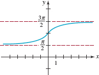
FIGURE 4.R.1 Graph for Problem 4

(a) y = f(x) - π

(b) y = f(x - 2)

(c) y = f(x + 3) + π/2

(d) y = -f(x)

(e) y = f(-x)

(f) y = 2f(x)

In Problems 5 and 6, use the graph of the one-to-one function f in Figure 4.R.I.

5. Give the domain and range of f^-1.

6. Sketch the graph of f^-1.

7. Express y = x – |x| + |x – 1| as a piecewise-defined function. Sketch the graph of the function.

8. Sketch the graph of the function Give the numbers at which the function is discontinuous.

In Problems 9 and 10, by examining the graph of the function f give the domain of the function g.

9.

10.

In Problems 11 and 12, the given function f is one-to-one. Find f ^-1.

11. f(x) = (x + 1)³

12. f(x) = x +

In Problems 13–16, compute for the given function.

13. f(x) = -3x² + 16x + 12

14. f(x) = x³ - x²

15.

16.

17. Area Express the area of the shaded region in Figure 4.R.2 as a function of h.

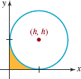
FIGURE 4.R.2 Circle in Problem 17

18. Parabolic Arch Determine a quadratic function that describes the parabolic arch shown in Figure 4.R.3.

FIGURE 4.R.3 Arch in Problem 18

19. Diameter of a Cube The diameter d of a cube is the distance between opposite vertices as shown in Figure 4.R.4. Express the diameter d as a function of the length 5 of a side of the cube. [Hint. First express the length y of the diagonal in terms of s.]

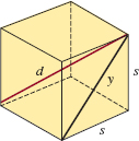
FIGURE 4.R.4 Cube in Problem 19

20. Inscribed Cylinder A circular cylinder of height h is inscribed in a sphere of radius 1 as shown in Figure 4.R.5. Express the volume of the cylinder as a function of h.

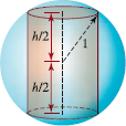
FIGURE 4.R.5 Inscribed cylinder in Problem 20

21. Distance from Home A baseball diamond is a square 90 ft on a side. See Figure 4.R.6. After a player hits a home run, he jogs around the bases at a rate of 6 ft/s.

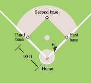
FIGURE 4.R.6 Baseball player in Problem 21

(a) As the player jogs between home base and first base, express his distance from home base as a function of time t, where t = 0 corresponds to the time he left home base—that is, 0 ≤ t ≤ 15.

(b) As the player jogs between home base and first base, express his distance from second base as a function of time t, where 0 ≤ t ≤ 15.

22. Area Again Consider the four circles shown in Figure 4.R.7. Express the area of the shaded region between them as a function of h.

FIGURE 4.R.7 Circles in Problem 22

23. Yet More Area The running track shown as the black curve in Figure 4.R.8 is to consist of two parallel straight parts and two congruent semicircular parts. The length of the track is to be 2 km. Express the area of the rectangular plot of land (the dark green rectangle) enclosed by the running track as a function of the radius of a semicircular end.

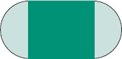
FIGURE 4.R.8 Running track in Problem 23

24. Cost of Construction A pipeline is to be constructed from a refinery across a swamp to storage tanks. See Figure 4.R.9. The cost of construction is $25,000 per mile over the swamp and $20,000 per mile over land. Express the cost of construction of the pipeline as a function of x shown in the figure.

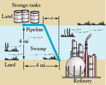
FIGURE 4.R.9 Pipeline in Problem 24

Foot notes

---

^*Not shown in (1) is the fact that the postage of a letter whose weight falls in the interval (3, 4] is determined by whether its weight falls in (3, 3.5] or (3.5, 4]. This is the only interval that is so divided.