
5. Polynomial and Rational Functions
In This Chapter
2.5 Division of Polynomial Functions
3.5 Zeros and Factors of Polynomial Functions
4.5 Real Zeros of Polynomial Functions

The curve formed by the cables holding up the roadway of a suspension bridge is described by a polynomial function.
A Bit of History The following problem perplexed mathematicians for centuries: For a general polynomial function f(x) = anxn + an-1 xn-1 +…+ a1x + a0 of degree n, find a formula, or a procedure, that expresses the zeros of f in terms of its coefficients. We saw in Chapter 004 that in the case of a second-degree (n = 2), or quadratic, polynomial, the zeros of f are expressed in terms of the coefficients by means of the quadratic formula. The problems for third-degree (n = 3) polynomials were solved in the sixteenth century through the pioneering work of the Italian mathematician Niccolò Fontana(1499-1557).
Around 1540 another Italian mathematician, Lodovico Ferrari (1522-1565), first discovered an algebraic formula for determining the zeros of fourth-degree (n = 4) polynomial functions. But for the next 284 years no one discovered any formulas for the zeros of general polynomials of degree n ≥ 5. For good reason! In 1824 the Norwegian mathematician Niels Henrik Abel (1802-1829) proved it was impossible to find such formulas for the zeros of all general polynomials of degrees n ≥ 5 in terms of their coefficients. Over the years it was assumed, but never proved, that a polynomial function / of degree n had at most n zeros. It was a truly outstanding achievement when the German mathematician Carl Friedrich Gauss (1777-1855) proved in 1799 that every polynomial function/ of degree n has exactly n zeros. As we will see in this chapter, these zeros may be real or complex numbers.
5.1 Polynomial Functions
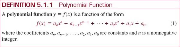
![]() Introduction In Chapter 004 we graphed functions such as y = 3, y = 2x — 1, y = 5x2 — 2x + 4, and y = x3. As we saw in the introduction to Section 4.3, these functions, in which the variable x is raised to nonnegative integer powers, are examples of a more general type of function called a polynomial function. Our goal in this section is to present some general guidelines for graphing such functions. But first we repeat the definition of a polynomial given in Section 4.3.
Introduction In Chapter 004 we graphed functions such as y = 3, y = 2x — 1, y = 5x2 — 2x + 4, and y = x3. As we saw in the introduction to Section 4.3, these functions, in which the variable x is raised to nonnegative integer powers, are examples of a more general type of function called a polynomial function. Our goal in this section is to present some general guidelines for graphing such functions. But first we repeat the definition of a polynomial given in Section 4.3.
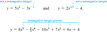
The domain of any polynomial function f is the set of all real numbers (— ∞, ∞). The following functions are not polynomials:
The function
is a polynomial, where we interpret the number 4 as the coefficient of x0. Since 0 is a nonnegative integer, a constant function such as y = 3 is a polynomial function since it is the same as y = 3x0.
![]() Terminology Polynomial functions are classified by their degree. The highest power of x in a polynomial is said to be its degree. So if an ≠ 0, then we say that f(x) in (1) has degree n. The number an in (1) is called the leading coefficient and a0 is called the constant term of the polynomial.
Terminology Polynomial functions are classified by their degree. The highest power of x in a polynomial is said to be its degree. So if an ≠ 0, then we say that f(x) in (1) has degree n. The number an in (1) is called the leading coefficient and a0 is called the constant term of the polynomial.
For example,
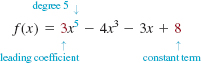
is a polynomial function of degree 5. We have already studied special polynomial functions in Section 4.3. Polynomial functions of degrees n = 0, n = 1, n = 2, and n = 3 are, respectively,
We considered linear and quadratic functions in Section 4.3. ![]()

Polynomials of degrees n = 4 and n = 5 are, in turn, commonly referred to as quartic and quintic functions. The constant function f(x) = 0 is called the zero polynomial.
![]() Graphs Recall, the graph of a constant function f(x) = a0 is a horizontal line, the graph of a linear function f(x) = a1x + a0, a1 ≠ 0, is a line with slope m = a1, and the graph of a quadratic function f (x) = a2x2 + a1x + a0, a2 ≠ 0, is a parabola.See Section 4.3. Such descriptive statements cannot be made about the graph of a higher- degree polynomial function. What is the shape of the graph of a fifth-degree polynomial function? It turns out that the graph of a polynomial function of degree n ≥ 3 can have several possible shapes. In general, graphing a polynomial function f of degree n ≥ 3 often demands the use of either calculus or a graphing utility. However, we will see in the discussion that follows that by determining
Graphs Recall, the graph of a constant function f(x) = a0 is a horizontal line, the graph of a linear function f(x) = a1x + a0, a1 ≠ 0, is a line with slope m = a1, and the graph of a quadratic function f (x) = a2x2 + a1x + a0, a2 ≠ 0, is a parabola.See Section 4.3. Such descriptive statements cannot be made about the graph of a higher- degree polynomial function. What is the shape of the graph of a fifth-degree polynomial function? It turns out that the graph of a polynomial function of degree n ≥ 3 can have several possible shapes. In general, graphing a polynomial function f of degree n ≥ 3 often demands the use of either calculus or a graphing utility. However, we will see in the discussion that follows that by determining

of the function we can, in some instances, quickly sketch a reasonable graph of a higher-degree polynomial function while keeping point plotting to a minimum. Before elaborating on each of these concepts we return to the notion of a power function first introduced in Section 4.2.
![]() See Section 1.6 for the definition of a monomial
See Section 1.6 for the definition of a monomial
![]() Power Function A special case of the power function is the single-term polynomial See Section 1.6 for the definition of a function or monomial,
Power Function A special case of the power function is the single-term polynomial See Section 1.6 for the definition of a function or monomial,
![]()
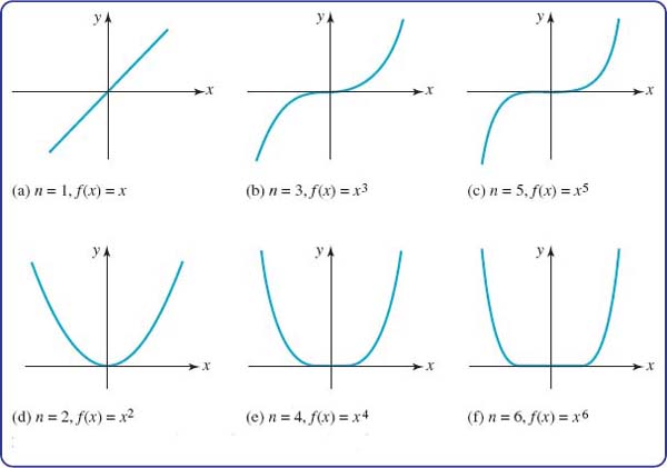
The graphs of (2) for degrees n = 1, 2, 3, 4, 5, and 6 are given in FIGURE 5.1.1. The interesting fact about (2) is that all the graphs for n odd are basically the same; the notable characteristics are that the graphs are symmetric about the origin and become increasingly flatter near the origin as the degree n increases. See Figures 5.1.1(a)-(c). A similar observation is true for the graphs of (2) for n even, except of course, the graphs are symmetric with respect to the y-axis. See Figures 5.1.1(d)-(f).
![]() Shifted Graphs Recall from Section 4.2 that for c > 0, the graphs of polynomial functions of the form
Shifted Graphs Recall from Section 4.2 that for c > 0, the graphs of polynomial functions of the form

can be obtained by vertical and horizontal shifts of the graph of y = axn. Also, if the leading coefficient a is positive, the graph of y = axn is either a vertical stretch or a vertical compression of the graph of the basic single-term polynomial function f(x) = xn. When a is negative we also carry out a reflection in the x-axis.
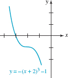
FIGURE 5.1.2 Reflected and shifted graph in Example 1

FIGURE 5.1.3 Mystery graph #1
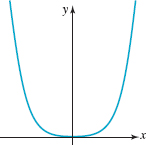
FIGURE 5.1.4 Mystery graph #2
EXAMPLE 1 Graphing a Shifted Polynomial Function
The graph of y = — (x + 2)3 — 1 is the graph of f(x) = x3 reflected in the x-axis, shifted 2 units to the left, and then shifted vertically downward 1 unit. First review Figure 5.1.1(b) and then see FIGURE 5.1.2.
![]() End Behavior The knowledge of the shape of a single-term polynomial function f(x) = xn is important for another reason. First, examine the computer-generated graphs given in FIGURES 5.1.3 and 5.1.4. Although the graph in FIGURE 5.1.3 certainly resembles the graphs in Figures 5.1.1(b) and 5.1.1(c), and the graph in FIGURE 5.1.4 resembles the graphs in Figures 5.1.1(d)—(f), the functions graphed in these two figures are not power functions f(x) = xn, n odd, or f(x) = xn, n even. We will not tell you at this point what the specific functions are except to say that they were both graphed on the interval [—1000, 1000]. The point is this: The function whose graph is given in FIGURE 5.1.3 could be almost any polynomial function
End Behavior The knowledge of the shape of a single-term polynomial function f(x) = xn is important for another reason. First, examine the computer-generated graphs given in FIGURES 5.1.3 and 5.1.4. Although the graph in FIGURE 5.1.3 certainly resembles the graphs in Figures 5.1.1(b) and 5.1.1(c), and the graph in FIGURE 5.1.4 resembles the graphs in Figures 5.1.1(d)—(f), the functions graphed in these two figures are not power functions f(x) = xn, n odd, or f(x) = xn, n even. We will not tell you at this point what the specific functions are except to say that they were both graphed on the interval [—1000, 1000]. The point is this: The function whose graph is given in FIGURE 5.1.3 could be almost any polynomial function
![]()
an > 0, of odd degree n, n = 3, 5,…when graphed on [— 1000, 1000]. Similarly, the graph in FIGURE 5.1.4 could be that of any polynomial function given in (1), with an > 0, of even degree n, n = 2, 4,…when graphed on a large interval around the origin. As the next theorem indicates, the terms enclosed in the colored rectangle in (3) are irrelevant when we look at a graph of a polynomial globally—that is, for values of |x| that are large. How a polynomial function f behaves when |x| is very large is said to be its end behavior. We will use the notation
x → -∞ and x → -∞
to indicate that the values of |x| are very large, or unbounded, in the negative and positive directions, respectively, on the number line.
To see why the graph of a polynomial function such as f (x) + -2x3 + 4x2 + 5 resembles the graph of the single-term polynomial y = -2x3 when |x| is large, let's factor out the highest power of x, that is, x3:

By letting |x| increase without bound, that is, x → -∞ or x → ∞, both 4/x and 5/x3 can be made as close to 0 as we want. Thus when the values of |x| are large, the values of the function f in (4) are closely approximated by the values of y = -2x3.
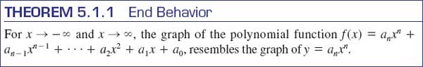
There can be only four types of end behavior for a polynomial function f. Although two of the end behaviors are already illustrated in Figures 5.1.3 and 5.1.4, we include them again in the pictorial summary given in FIGURE 5.1.5. To interpret the red arrows in FIGURE 5.1.5 let's examine Figure 5.1.5(a). The position and direction of the left arrow (left arrow points down) indicates that as x → -∞, the values f (x) are negative and large in magnitude. Stated another way, the graph is heading downward as x → -∞. Similarly, the position and direction of the right arrow (right arrow points up) indicates that the graph is heading upward as x → ∞.
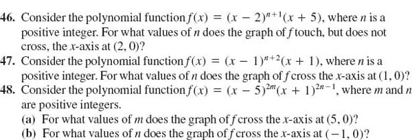
FIGURE 5.1.5 End behavior of a polynomial function f depends on its degree n and on the sign of its leading coefficient an
![]() Local Behavior The gaps between the arrows in FIGURE 5.1.5 correspond to some interval around the origin. In these gaps the graph of f exhibits local behavior; in other words, the graph of f shows the characteristics of a polynomial function of a particular degree. This local behavior includes the x- and y-intercepts of the graph, the behavior of the graph at an x-intercept, the turning points of the graph, and observable symmetry of the graph (if any). A turning point is a point (c, f(c)) at which the graph of a polynomial function f changes direction; that is, the function f changes from increasing to decreasing or vice versa. The graph of a polynomial function of degree n can have up to n — 1 turning points. In calculus a turning point corresponds to a relative, or local, extremum off. A relative extremum is classified as either a maximum or a minimum. If (cf(c)) is a turning point, then in some neighborhood of x = c, f (c) is either the largest (relative maximum) or smallest (relative minimum) function value. If f(c) is a relative maximum, then at (c, f(c)) the graph of a polynomial functionf must change from increasing immediately to the left of x = c to decreasing immediately to the right of x = c, whereas iff(c) is a relative minimum, then at (c, f (c)) the function f changes from decreasing to increasing. These concepts are illustrated in Example 2.
Local Behavior The gaps between the arrows in FIGURE 5.1.5 correspond to some interval around the origin. In these gaps the graph of f exhibits local behavior; in other words, the graph of f shows the characteristics of a polynomial function of a particular degree. This local behavior includes the x- and y-intercepts of the graph, the behavior of the graph at an x-intercept, the turning points of the graph, and observable symmetry of the graph (if any). A turning point is a point (c, f(c)) at which the graph of a polynomial function f changes direction; that is, the function f changes from increasing to decreasing or vice versa. The graph of a polynomial function of degree n can have up to n — 1 turning points. In calculus a turning point corresponds to a relative, or local, extremum off. A relative extremum is classified as either a maximum or a minimum. If (cf(c)) is a turning point, then in some neighborhood of x = c, f (c) is either the largest (relative maximum) or smallest (relative minimum) function value. If f(c) is a relative maximum, then at (c, f(c)) the graph of a polynomial functionf must change from increasing immediately to the left of x = c to decreasing immediately to the right of x = c, whereas iff(c) is a relative minimum, then at (c, f (c)) the function f changes from decreasing to increasing. These concepts are illustrated in Example 2.
![]() Symmetry It is easy to tell by inspection those polynomial functions whose graphs possess symmetry with respect to either the y-axis or the origin. The words even and odd functions have special meaning for polynomial functions. Recall, an even function is one for which f (—x) = f (x) and an odd function is one for which f (— x) = —f (x). These two conditions hold for polynomial functions in which the powers of x are all even integers and all odd integers, respectively. For example,
Symmetry It is easy to tell by inspection those polynomial functions whose graphs possess symmetry with respect to either the y-axis or the origin. The words even and odd functions have special meaning for polynomial functions. Recall, an even function is one for which f (—x) = f (x) and an odd function is one for which f (— x) = —f (x). These two conditions hold for polynomial functions in which the powers of x are all even integers and all odd integers, respectively. For example,

A function such as f(x) 5 3x6 - x4 + 6 is an even function because the obvious powers are even integers; the constant term 6 is actually 6x0 and 0 is an even nonnegative integer.
![]() Intercepts The graph of every polynomial function f passes through the y-axis since x = 0 is the domain of the function. The y-intercept is the point Recall, a number c is a zero of a function f if f (c) = 0 In this discussion we assume c is a real zero. If x - C is a factor of a polynomial function f, that is, where f (x) 5 (x 2 c)q(x), where q(x) is another polynomial, then clearly f(c) = 0 and the corresponding point on the graph is (c,0) Thus the real zeros of a polynomial function are the x-coordinates of the x-intercepts of its graph. If (x - c)m is a factor of f, where m > 1 is a positive integer, and (x - c)m+1 is not a factor of f, then c is said to be a repeated zero, or more precisely, a zero of multiplicity m. For example, f (x) 5 x2 2 10x + 25 is equivalent to f (x) = (x - 5)2. Hence 5 is a repeated zero or a zero of multiplicity 2. When m = 1 c is called a simple zero. For example,
Intercepts The graph of every polynomial function f passes through the y-axis since x = 0 is the domain of the function. The y-intercept is the point Recall, a number c is a zero of a function f if f (c) = 0 In this discussion we assume c is a real zero. If x - C is a factor of a polynomial function f, that is, where f (x) 5 (x 2 c)q(x), where q(x) is another polynomial, then clearly f(c) = 0 and the corresponding point on the graph is (c,0) Thus the real zeros of a polynomial function are the x-coordinates of the x-intercepts of its graph. If (x - c)m is a factor of f, where m > 1 is a positive integer, and (x - c)m+1 is not a factor of f, then c is said to be a repeated zero, or more precisely, a zero of multiplicity m. For example, f (x) 5 x2 2 10x + 25 is equivalent to f (x) = (x - 5)2. Hence 5 is a repeated zero or a zero of multiplicity 2. When m = 1 c is called a simple zero. For example, ![]() and
and ![]() are simple zeros of f (x) = 6x2 - x - 1 since f can be written as
are simple zeros of f (x) = 6x2 - x - 1 since f can be written as ![]() The behavior of the graph of f at an x-intercept (c, 0) depends on whether c is a simple zero, or a zero of multiplicity m > 1 where m is either an even or an odd integer.
The behavior of the graph of f at an x-intercept (c, 0) depends on whether c is a simple zero, or a zero of multiplicity m > 1 where m is either an even or an odd integer.
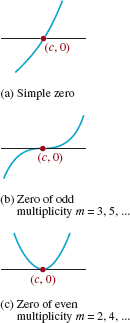
FIGURE 5.1.6 x-intercepts of a polynomial function f(x) with a positive leading coefficient

In the case when c is either a simple zero or a zero of odd multiplicity m = 3,5,…, f (x) changes sign at (c, 0), whereas if c is a zero of even multiplicity m = 2, 4,…, f (x) does not change sign at We note that in FIGURE 5.1.6 we have assumed that the polynomial function f has a positive leading coefficient. If the sign of the leading coefficient of f is negative, then the graphs in FIGURE 5.1.6 would be reflected in the x-axis. For example, at a zero of even multiplicity and negative leading coefficient the graph of f would be tangent to the x-axis from below that axis.
EXAMPLE 2 Graphing a Polynomial Function
Graph f (x) = x3 - 9x.
Solution Here are some of the things that we look at to sketch the graph of f.
End Behavior: By ignoring all terms but the first, we see that the graph of f resembles the graph of y = x3 for large|x|. That is, the graph goes down to the left as x → - ∞ and up to the right as x → ∞, as illustrated in Figure 5.1.5(a).
Symmetry: Since all the powers are odd integers, f is an odd function. The graph of f is symmetric with respect to the origin.
Intercepts: f (0) = 0 and so the y-intercept is (0, 0). Setting f(x) = 0we see that we must solve x3 - 9x = 0. Factoring,
![]()
shows that the zeros of f are x = 0 and ![]() . The x-intercepts are (0, 0), (-3, 0), and (3, 0).
. The x-intercepts are (0, 0), (-3, 0), and (3, 0).
The Graph: From left to right, the graph rises (f is increasing) from the third quadrant and passes straight through (- 3, 0) since -3 is a simple zero. Although the graph is rising as it passes through this intercept it must turn back downward (f decreasing) at some point in the second quadrant to get through the intercept (0, 0). Since the graph is symmetric with respect to the origin, its behavior is just the opposite in the first and fourth quadrants. See FIGURE 5.1.7.
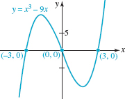
FIGURE 5.1.7 Graph of function in Example 2
In Example 2, the graph of f has two turning points. On the interval [-3, 0] there is a relative maximum and on the interval [0, 3] there is a relative minimum. We made no attempt to locate the corresponding turning points precisely; this is something that would, in general, require techniques from calculus. The best we can do using precalculus mathematics to refine the graph is to resort to plotting additional points on the intervals of interest. By the way, f (x) = x3 - 9x is the function whose graph on the interval [-1000, 1000] is given in FIGURE 5.1.3.
EXAMPLE 3 Graphing a Polynomial Function
Graph f (x) = (1 - x)(x + 1)2.
Solution Multiplying out, f is the same as f (x) = -x3 - x2 1 x + 1.
End Behavior: From the preceding line we see that the graph of f resembles the graph of y = -x3 for large | x |, just the opposite of the end behavior of the function in Example 1. See Figure 5.1.5(b).
Symmetry: As we see from f (x) = -x3 - x2 + x + 1, there are both even and odd powers of x present. Hence f is neither even nor odd; its graph possesses no y- axis or origin symmetry.
Intercepts: f(0) = 1 so the y-intercept is (0, 1).From the original factored form of the function f(x), we see that (-1, 0) and (1, 0) are the x-intercepts of its graph.
The Graph: From left to right, the graph falls (f decreasing) from the second quadrant and then, because -1 is a zero of multiplicity 2, the graph is tangent to the x-axis at (-1, 0). The graph then rises (f increasing) as it passes through the y-intercept (0, 1). At some point within the interval [-1, 1] the graph turns downward (f decreasing) and, since 1 is a simple zero, passes through the x-axis at (1, 0) heading downward into the fourth quadrant. See FIGURE 5.1.8.
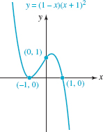
FIGURE 5.1.8 Graph of function in Example 3
In Example 3, there are again two turning points. It should be clear that the point (— 1, 0) is a turning point (f changes from decreasing to increasing at this point) and f (— 1) = 0 is a relative minimum of f. There is a turning point (f changes from increasing to decreasing at this point) on the interval [—1, 1] and corresponds to a relative maximum of f.
EXAMPLE 4 Zeros of Multiplicity Two
Graph f (x) = x4 — 4x2 + 4.
Solution Before proceeding, note that the right-hand side of f is a perfect square. That is, f (x) = (x2 — 2)2. Since ![]() by the laws of exponents we can write
by the laws of exponents we can write
![]()
End Behavior. Inspection of f (x) shows that its graph resembles the graph of y = x4 for large |x|. That is, the graph goes up to the left as x → -∞ and up to the right as x → ∞ as shown in Figure 5.1.5(c).
Symmetry: Because f (x) contains only even powers of x, it is an even function and so its graph is symmetric with respect to the y-axis.
Intercepts: f (0) = 4 so the y-intercept is (0, 4). Inspection of (5) shows the x-intercepts are ![]() and
and ![]() .
.
The Graph: From left to right, the graph falls from the second quadrant and then, because ![]() is a zero of multiplicity 2, the graph touches the x-axis at
is a zero of multiplicity 2, the graph touches the x-axis at ![]() . The graph then rises from this point to the y-intercept (0, 4). We then use the y-axis symmetry to finish the graph in the first quadrant. See FIGURE 5.1.9.
. The graph then rises from this point to the y-intercept (0, 4). We then use the y-axis symmetry to finish the graph in the first quadrant. See FIGURE 5.1.9.
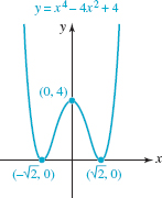
FIGURE 5.1.9 Graph of function in Example 4
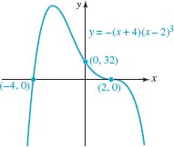
FIGURE 5.1.10 Graph of function in Example 5
In Example 4, the graph of f has three turning points. From the even multiplicity of the zeros, along with the y-axis symmetry, it can be deduced that the x-intercepts ![]() and
and ![]() are turning points and f (
are turning points and f (![]() ) = 0and f (
) = 0and f (![]() ) = 0 are relative minima, and that the y-intercept (0, 4) is a turning point and f (0) = 4 is a relative maximum.
) = 0 are relative minima, and that the y-intercept (0, 4) is a turning point and f (0) = 4 is a relative maximum.
EXAMPLE 5 Zeros of Multiplicity Three
Graph f (x) = — (x + 4)(x — 2)3.
Soultion
End Behavior. Inspection of f shows that its graph resembles the graph of y = —x4for large |x|. This end behavior of f is shown in Figure 5.1.5(d).
Symmetry: The function f is neither even nor odd. It is straightforward to show that f(—x) ≠ f(x) and f(— x) ≠ —f(x).
Intercepts: f(0) = (—4)(—2)3 = 32 so the y-intercept is (0, 32).From the factored form of f (x), we see that (—4, 0) and (2, 0) are the x-intercepts.
The Graph: From left to right, the graph rises from the third quadrant and then, because -4 is a simple zero, the graph of f passes directly through the x-axis at (—4, 0). Some where within the interval [—4, 0] the function f must change from increasing to decreasing to enable its graph to pass through the y-intercept (0, 32). After its graph passes through the y-intercept, the function f continues to decrease but, since 2 is a zero of multiplicity 3, its graph flattens as it passes through (2, 0) heading downward into the fourth quadrant. See FIGURE 5.1.10.
Note in Example 5 that since f is of degree 4, its graph could have up to three turning points. But as can be seen from FIGURE 5.1.10, the graph of f possesses only one turning point and corresponds to a relative maximum of f.

FIGURE 5.1.11 Graph of function in Example 6
EXAMPLE 6 Zeros of Multiplicity Two and Three
Graph f(x) = (x - 3)(x - 1)2(x + 2)3.
Solution The function f is of degree 6 and so its end behavior resembles the graph of y = x6 for large |x| . See Figure 5.1.5(c). Also, the function f is neither even nor odd; its graph possesses no y-axis or origin symmetry. The y-intercept is (0, f(0)) = (0, -24). From the factors of / we see that x-intercepts of the graph are (-2, 0), (1, 0), and (3, 0). Since -2 is a zero of multiplicity 3, the graph of f is flattened as it passes through the point (-2, 0). Since 1 is a zero of multiplicity 2, the graph of f is tangent to the x-axis at (1, 0). Since 3 is a simple zero, the graph of/passes directly through the x-axis at (3, 0). Putting all these facts together we obtain the graph in FIGURE 5.1.11.
In Example 6, since the function f is of degree 6 its graph could have up to five turning points. But as the graph in FIGURE 5.1.11 shows there are only three turning points. Two of these points correspond to relative minima and at the remaining point (1, 0), f (1) = 0is a relative maximum.
5.1 ExercisesAnswers to selected odd-numbered problems begin on page ANS-12.
In Problems 1-8, proceed as in Example 1 and use transformations to sketch the graph of the given polynomial function.

In Problems 9-12, determine whether the given polynomial function f is even, odd, or neither even nor odd. Do not graph.
![]()
In Problems 13-18, match the given graph with one of the polynomial functions in (a)-(f).
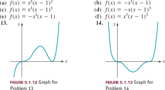

FIGURE 5.1.14 Graph for Problem 15

FIGURE 5.1.14 Graph for Problem 16

FIGURE 5.1.14 Graph for Problem 17

FIGURE 5.1.14 Graph for Problem 18
In Problems 19-40, proceed as in Example 2 and sketch the graph of the given polynomialfunction f.
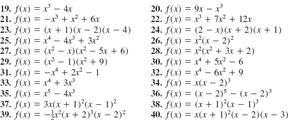
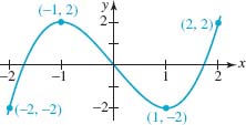
FIGURE 5.1.18 Graph for Problem 41
FIGURE 5.1.19 Graph for Problem 42

Miscellaneous Applications
Constructing a Box An open box can be made from a rectangular piece of cardboard by cutting a square of length x from each corner and bending up the sides. See FIGURE 5.1.20. If the cardboard measures 30-cm by 40-cm, show that the volume of the resulting box is given by
V(x) = x(30 — 2x)(40 — 2x).
Sketch the graph of V(x) for x > 0. What is the domain of the function V?
Another Box In order to hold its shape, the box in Problem 49 will require tape or some other fastener at the corners. An open box that holds itself together can be made by cutting out a square of length x from each corner of a rectangular piece of cardboard, cutting on the solid line, and folding on the dashed lines, as shown in FIGURE 5.1.21. Find a polynomial function V(x) that gives the volume of the resulting box if the original cardboard measures 30-cm by 40-cm. Sketch the graph of V(x) for x > 0.
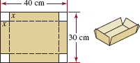
FIGURE 5.1.20 Box in Problem 49

FIGURE 5.1.21 Box in Problem 50
For Discussion
51. Examine FIGURE 5.1.5. Then discuss whether there can exist cubic polynomial functions that have no real zeros.
52. Suppose a polynomial function f has three zeros, —3, 2, and 4, and has the end behavior that its graph goes down to the left as x → —∞ and down to the right as x → ∞. Discuss possible equations for f.
Calculator/Computer Problems
In Problems 53 and 54, use a graphing utility to examine the graph of the given polynomial function on the indicated intervals.
53. f(x) = — (x — 8)(x + 10)2; [— 15, 15], [— 100, 100], [— 1000, 1000]
54. f(x) = (x — 5)2(x + 5)2; [— 10, 10], [— 100, 100], [— 1000, 1000]
5.2 Division of Polynomial Functions
![]() Introduction In this section we will see that the method for dividing two polynomial functions f (x) and g(x) is quite similar to division of positive integers. Moreover, division of a polynomial function f (x) by a linear polynomial g (x) = x - c is particularly useful because it provides us with a way of evaluating the function f at the number c without having to compute any powers of c.
Introduction In this section we will see that the method for dividing two polynomial functions f (x) and g(x) is quite similar to division of positive integers. Moreover, division of a polynomial function f (x) by a linear polynomial g (x) = x - c is particularly useful because it provides us with a way of evaluating the function f at the number c without having to compute any powers of c.
We begin with a review of the terminology of fractions.
![]() Terminology If p > 0 and s > 0 are integers such that p ≥ s, then p/s is called an improper fraction. By dividing p by s, we obtain unique integers q and r that satisfy
Terminology If p > 0 and s > 0 are integers such that p ≥ s, then p/s is called an improper fraction. By dividing p by s, we obtain unique integers q and r that satisfy
![]()
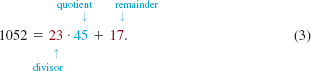
where 0 ≤ r < s. The number p is called the dividend, s is the divisor, q is the quotient, and r is the remainder. For example, consider the improper fraction ![]() Performing long division gives
Performing long division gives

The result in (2) can be written as ![]() where
where ![]() is a proper fraction since the numerator is less than the denominator, in other words, the fraction is less than 1. If we multiply this result by the divisor 23 we obtain the special way of writing the dividend m illustrated in the second equation in (1):
is a proper fraction since the numerator is less than the denominator, in other words, the fraction is less than 1. If we multiply this result by the divisor 23 we obtain the special way of writing the dividend m illustrated in the second equation in (1):
![]() Division of Polynomials If the degree of a polynomial f(x) is greater than or equal to the degree of the polynomial g(x), then f(x)/g (x) is also called an improper fraction. A result analogous to (1) is called the Division Algorithm for polynomials.
Division of Polynomials If the degree of a polynomial f(x) is greater than or equal to the degree of the polynomial g(x), then f(x)/g (x) is also called an improper fraction. A result analogous to (1) is called the Division Algorithm for polynomials.

The polynomial f(x) is called the dividend, g(x) the divisor, q(x) the quotient, and r(x) the remainder. Because r(x) has degree less than the degree of g(x), the rational expression r(x)/g(x) is called a proper fraction.
Observe in (4) when r(x) = 0, then f(x) = g(x)q(x) and so the divisor g(x) is a factor of f (x). In this case, we say thatf (x) is divisible by g(x) or, in older terminology, g(x) divides evenly into f(x).
EXAMPLE 1 Division of Two Polynomials
Use long division to find the quotient q(x) and remainder r(x) when the polynomial f (x) = 3x3 - x2 - 2x + 6 is divided by the polynomial g(x) = x2 + 1.
Solution By long division,
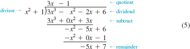
The result of the division (5) can be written
![]()
Thus the quotient is 3x - 1 and the remainder is -5x + 7. If we multiply both sides of the last equation by the divisor x2 + 1 we get the second form given in (4):
![]()
If the divisor g(x) is a linear polynomial x - c, it follows from the Division Algorithm that the degree of the remainder r is 0, that is to say, r is a constant. Thus (4) becomes
![]()
When the number x = c is substituted into (7), we discover an alternative way of evaluating a polynomial function:
![]()
The foregoing result is called the Remainder Theorem.

EXAMPLE 2 Finding the Remainder
Use the Remainder Theorem to find r when f (x) = 4x3 - x2 + 4 is divided by x - 2.
Solution From the Remainder Theorem the remainder r is the value of the function f evaluated at x = 2:
![]()
Example 2, where a remainder r is determined by calculating a function value f(c), is more interesting than important. What is important is the reverse problem: Determine the function value f(c) by finding the remainder r by division of f by x - c. The next two examples illustrate this concept.
EXAMPLE 3 Evaluation by Division
Use the Remainder Theorem to find f(c) for f (x) = x5 - 4x3 + 2x - 10 when c = -3.
Solution The value f (-3) is the remainder when f(x) = x5 - 4x3 + 2x - 10 is divided by x - (-3) = x + 3. For the purposes of long division we must account for the missing x4 and x2 terms by rewriting the dividend as
f (x) = x5 + 0x4 - 4x3 + 0x2 + 2x - 10.
Then,
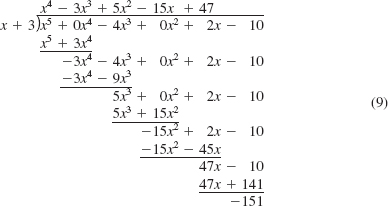
The remainder r in the division is the value of the function f at x = -3, that is, f (-3) = -151.
![]() Synthetic Division After working through Example 3 one could justifiably ask the question: Why would anyone want to calculate the value of a polynomial function f by division? The answer is: We would not bother to do this were it not for synthetic division. Synthetic division is a shorthand method of dividing a polynomial f (x) by a linear polynomial x - c; it does not require writing down the various powers of the variable x but only the coefficients of these powers in the dividend f (x) (which must include all 0 coefficients). It is also a very efficient and quick way of evaluating f(c) since the process utilizes only the arithmetic operations of multiplication and addition. No exponentiations such as 23 and 22 in (8) are involved.
Synthetic Division After working through Example 3 one could justifiably ask the question: Why would anyone want to calculate the value of a polynomial function f by division? The answer is: We would not bother to do this were it not for synthetic division. Synthetic division is a shorthand method of dividing a polynomial f (x) by a linear polynomial x - c; it does not require writing down the various powers of the variable x but only the coefficients of these powers in the dividend f (x) (which must include all 0 coefficients). It is also a very efficient and quick way of evaluating f(c) since the process utilizes only the arithmetic operations of multiplication and addition. No exponentiations such as 23 and 22 in (8) are involved.
For example, consider the long division:
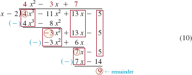
We can make several observations about (10):
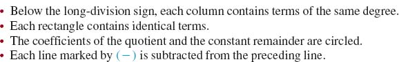
If we delete variables and the observed repetitions in (10), we have

As indicated by the arrows in (11), this can be written more compactly as
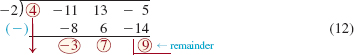
If we bring down the leading coefficient 4 of the dividend, as indicated by the red arrow in (12), then the coefficients of the quotient and remainder are on one line.
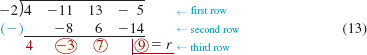
Now observe that each number in the second row of (13) can be found by multiplying the number in the third row of the preceding column by - 2, and that each number in the third row is obtained by subtracting each number in the second row from the corresponding number in the first row.
Finally, we can avoid the subtraction in (13) by multiplying by +2 (the additive inverse of -2) and adding the second row to the first. This is illustrated below:
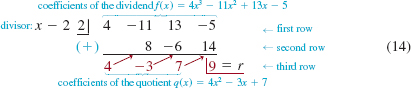
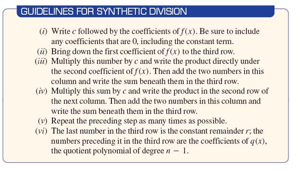
The procedure of synthetic division for dividing f (x), a polynomial of degree n > 0, by x - c is summarized as follow:
EXAMPLE 4 Example 3 Revisited
Use synthetic division to divide f(x) = x45 - 4x3 + 2x - 10 when x + 3.
Solution The synthetic division of f by x + 3 = x - (-3) is

The quotient is the fourth-degree polynomial q(x) = x4 - 3x3 + 5x2 - 15x + 47 andthe constant remainder is r = -151. Also, the value of the function f at -3 is the remainder f(-3) = -151.
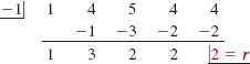
EXAMPLE 5 Using Synthetic Division to Evaluate a Function
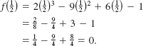
Use the Remainder Theorem to find f (2) for
Using synthetic division we can find f(2) without computing the powers of 2: 26, 25, 24, 23, and 22. ![]()
f(x) = -3x6 + 4x5 + x4 - 8x3 - 6x2 + 9.
Solution We will use synthetic division to find the remainder r in the division of f by x - 2. We begin by writing down all the coefficients in f(x), including 0 as the coefficient of x. From
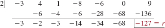
we see that f (2) = -127.
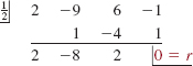
EXAMPLE 6 Using Synthetic Division to Evaluate a Function
Use synthetic division to evaluate f (x) = x3 - 7x2 + 13x - 15 at x = 5.
Solution From the synthetic division

we see that f (5) = 0.
The result in Example 6 that f (5) = 0 shows that 5 is a zero of the given function f. Moreover, we have found additionally that f is evenly divisible by the linear polynomial x - 5, or put another way, x - 5 is a factor of f. The synthetic division shows that f (x) = x3 - 7x2 + 13x - 15 is equivalent to
f(x) = (x - 5)(x2 - 2x + 3).
In the next section we will further explore the use of the Division Algorithm and Remainder Theorem as a help in finding zeros and factors of a polynomial function.

In Problems 1-10, use long division to find the quotient q (x) and remainder r (x) when the polynomial f (x) is divided by the given polynomial g(x). In each case write your answer in the form f (x) = g(x)q(x) + r(x).
f (x) = 8x2 + 4x - 7; g(x) = x2
f (x) = x2 + 2x - 3; g(x) = x2 + 1
f (x) = 5x3 - 7x2 + 4x + 1; g(x) = x2 + x - 1
f (x) = 14x3 - 12x2 + 6; g(x) = x2 - 1
f (x) = 2x3 + 4x2 - 3x + 5; g(x) = (x + 2)2
f (x) = x3 + x2 + x + 1;g(x) = (2x + 1)2
f (x) = 27x3 + x - 2; g(x) = 3x2 - x
f (x) = x4 + 8; g(x) = x3 + 2x - 1
f (x) = 6x5 + 4x4 + x3; g(x) = x3 - 2
f (x) = 5x6 - x5 + 10x4 + 3x2 - 2x + 4; g(x) = x2 + x - 1
In Problems 11-16, proceed as in Example 2 and use the Remainder Theorem to find r when f(x) is divided by the given linear polynomial.
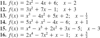
In Problems 17-22, proceed as in Example 3 and use the Remainder Theorem to find f (c) for the given value of c.
In Problems 23-32, use synthetic division to find the quotient q(x) and remainder r(x) when f(x) is divided by the given linear polynomial.

In Problems 33-38, use synthetic division and the Remainder Theorem to find f (c) for the given value of c.
33. f (x) = 4x2 - 2x + 9; c = -3
34. ![]()
35. f(x) = 14x4 - 60x3 + 49x2 - 21x + 19; c = 1
36. f(x) = 3x5 1 x2 - 16; c = -2
37. f(x) = 2x6 - 3x5 1 x4 - 2x + 1; c = 4
38. f(x) = x1 - 3x5 + 2x3 - x + 10; c = 5
In Problems 39 and 40, use long division to find a value of k such that f (x) is divisible by g (x).
39. f(x) = x4 + x3 + 3x2 + kx - 4; g(x) = x2 - 1
40. f (x) = x5 - 3x4 + 7x3 1 kx2 1 9x - 5; g(x) = x2 - x + 1
In Problems 41 and 42, use synthetic division to find a value of k such that f(x) is divisible by g(x).
41. f(x) = kx4 + 2x2 + 9k; g(x) = x - 1
42. f (x) = x3 + kx2 - 2kx + 4; g(x) = x + 2
43. Find a value of k such that the remainder in the division of f (x) = 3x2 - 4kx + 1 by g(x) = x + 3 is r = -20.
44. When f (x) = x2 - 3x - 1 is divided by x - c, the remainder is r = 3. Determine c.
5.3 Zeros and Factors of Polynomial Functions
![]() Introduction In Section 4.1 we saw that a zero of a function f is a number c for which f (c) = 0. A zero c of a function f can be a real or a complex number. Recall from Section 2.4 that a complex number is a number of the form z = a + bi, where i2 = -1, and a and b are real numbers. The number a is called the real part of z and b is called the imaginary part of z. The symbol i is called the imaginary unit and it is common practice to write it as
Introduction In Section 4.1 we saw that a zero of a function f is a number c for which f (c) = 0. A zero c of a function f can be a real or a complex number. Recall from Section 2.4 that a complex number is a number of the form z = a + bi, where i2 = -1, and a and b are real numbers. The number a is called the real part of z and b is called the imaginary part of z. The symbol i is called the imaginary unit and it is common practice to write it as ![]() . If z = a + bi is a complex number, then
. If z = a + bi is a complex number, then ![]() is called its conjugate. Thus the simple polynomial function f (x) = x2 + 1 has two complex zeros since the solutions of x2 + 1 = 0 are
is called its conjugate. Thus the simple polynomial function f (x) = x2 + 1 has two complex zeros since the solutions of x2 + 1 = 0 are ![]() that is, i and - i.
that is, i and - i.
In this section we explore the connection between the zeros of a polynomial function f, the operation of division, and the factors of f.
EXAMPLE 1 A Real Zero
Consider the polynomial function f(x) = 2x3 - 9x2 + 6x - 1.The real number ![]() is a zero of the function since
is a zero of the function since
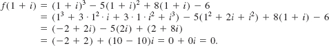
EXAMPLE 2 A Complex Zero
Consider the polynomial function f(x) = x3 - 5x2 + 8x - 6. The complex number 1 + i is a zero of the function. To verify this we use the binomial expansion of (a = b)3 and the fact that i2 = -1 and i3 = - 1:
See (4) in Section 1.6.![]()
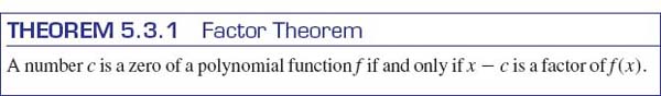
![]() Factor Theorem We can now relate the notion of a zero of a polynomial function f with division of polynomials. From the Remainder Theorem we know that when f(x) is divided by the linear polynomial x - c the remainder is r = f (c). If c is a zero off, then f(c) = 0 implies r = 0. From the form of the Division Algorithm given in (4) of Section 5.2 we can then write f as
Factor Theorem We can now relate the notion of a zero of a polynomial function f with division of polynomials. From the Remainder Theorem we know that when f(x) is divided by the linear polynomial x - c the remainder is r = f (c). If c is a zero off, then f(c) = 0 implies r = 0. From the form of the Division Algorithm given in (4) of Section 5.2 we can then write f as
![]()
Thus, if c is a zero of a polynomial functionf, then x - c is a factor of f (x). Conversely, if x - c is a factor of f (x), then f has the form given in (1). In this case, we see immediately that f(c) = (c - c)q(c) = 0. These results are summarized in the Factor Theorem given next.
If a polynomial function f is of degree n and (x - c)m, m ≤ n, is a factor of f (x), then c is said to be a zero of multiplicity m. When m = 1, c is a simple zero. Equivalently, we say that the number c is a root of multiplicity m of the equation f(x) = 0. We have already examined the graphical significance of simple and repeated real zeros of a polynomial function f in Section 5.1. See FIGURE 5.1.6.
EXAMPLE 3 Factors of a Polynomial
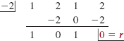
Determine whether
(a) x + 1 is a factor of f(x) = x4 - 5x2 + 6x - 1,
(b) x - 2 is a factor of f(x) = x3 - 3x2 + 4.
Solution We use synthetic division to divide f(x) by the given linear term.
(a) From the division

we see that f(- 1)= -11 ≠ 0 and so -1 is not a zero of f. We conclude that x-(-1)=x+1 is not a factor of f(x).
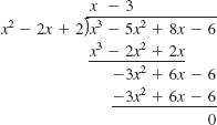
(b) From the division
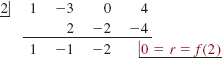
we see that f(2)=0 This means that 2 is a zero and that x - 2 is a factor of f(x) From the division we see that the quotient is q(x) = x2 - x - 2 and so f(x) = (x - 2)(x2 - x - 2).
![]() Number of Zeros In Example 6 of Section 5.1 we graphed the polynomial function
Number of Zeros In Example 6 of Section 5.1 we graphed the polynomial function
![]()
The number 3 is a zero of multiplicity 1, or a simple zero off, the number 1 is a zero of multiplicity 2, and -2 is a zero of multiplicity 3. Although the function f has three distinct zeros (different from one another), nevertheless, it is standard practice to say that f has six zeros because we count the multiplicities of each zero. Hence for the function f in (2), the number of zeros is 1 + 2 + 3 = 6. The question
How many zeros does a polynomial function f have?
is answered next.
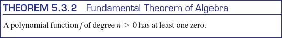
Theorem 5.3.2, first proved by the German mathematician Carl Friedrich Gauss(1777-1855) in 1799, is considered one of the major milestones in the history of mathematics. At first reading, this theorem does not appear to say much, but when combined with the Factor Theorem, the Fundamental Theorem of Algebra shows:
![]()
Of course if a zero is repeated, say it has multiplicity k, we count that zero k times. To prove (3), we know from the Fundamental Theorem of Algebra thatf has a zero; call it c1. By the Factor Theorem we can write
![]()
where q1 is a polynomial function of degree n - 1. If n - 1 ≠ 0, then in like manner we know that q1 must have a zero; call it c2 and so (4) becomes
![]()
where q2 is a polynomial function of degree n - 2. If n - 2 ≠ 0, we continue and arrive at
![]()
and so on. Eventually we arrive at a factorization of f(x) with n linear factors and the last factor qn(x) is of degree 0. In other words, qn (x) = an, where an is a constant—specifically, an is the leading coefficient of f. We have arrived at the complete factorization of f(x).

Bear in mind that some or all the zeros c1,…, cn in (6) may be complex numbers a + bi, where b ≠ 0.
In the case of a second-degree, or quadratic, polynomial function f(x) = ax2 + bx + c, where the coefficients a, b, and c are real numbers, the zeros c1and c2 of f can be found using the quadratic formula:
![]()
The results in (7) tell the whole story about the zeros of the quadratic function:
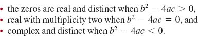
It follows from (6) that the complete linear factorization of a quadratic polynomial function f (x) = ax2 + bx + c is
![]()
EXAMPLE 4 Example 1 Revisited
In Example 1 we demonstrated that ![]() is a zero of f(x) = 2x3 - 9x2 + 6x - 1.We now know that
is a zero of f(x) = 2x3 - 9x2 + 6x - 1.We now know that ![]() is a factor of f(x) and that f(x) has three zeros. The synthetic division
is a factor of f(x) and that f(x) has three zeros. The synthetic division
again demonstrates that ![]() is a zero of f(x) (the 0 remainder is the value of
is a zero of f(x) (the 0 remainder is the value of ![]() and, additionally, gives us the quotient q(x) obtained in the division of f(x) by
and, additionally, gives us the quotient q(x) obtained in the division of f(x) by ![]() that is,
that is, ![]() As shown in (8) we can now factor the quadratic quotient q (x) = 2x2 - 8x + 2 by finding the roots of 2x2 - 8x + 2 = 0 from the quadratic formula:
As shown in (8) we can now factor the quadratic quotient q (x) = 2x2 - 8x + 2 by finding the roots of 2x2 - 8x + 2 = 0 from the quadratic formula:
Thus the remaining zeros of f(x) are the irrational numbers ![]() and
and ![]() . With the identification of the leading coefficient as a3 = 2, it follows from (8) that the complete linear factorization of f(x) is then
. With the identification of the leading coefficient as a3 = 2, it follows from (8) that the complete linear factorization of f(x) is then
![]()
EXAMPLE 5 Using Synthetic Division
Find the complete linear factorization of
![]()
given that 1 is a zero of f of multiplicity two.
Solution We know that x - 1 is a factor of f (x) so by the division

we find ![]()
Since 1 is a zero of multiplicity 2, x - 1 must also be a factor of the quotient q(x) = x3 - 11x2 + 36x - 26. By the division,

we conclude that q(x) can be written = (x - 1)(x2 - 10x + 26). Therefore,
![]()
The remaining two zeros, found by solving x2 - 10x + 26 = 0 by the quadratic formula, are the complex numbers 5 + i and 5 - i. Since the leading coefficient is a4 = 1 the complete linear factorization of f(x) is
![]()
EXAMPLE 6 Finding a Polynomial Function
Find a polynomial function f of degree 3, with zeros 1, - 4, and 5 such that its graph possesses the y-intercept (0, 5).
Solution Because we have three zeros 1, - 4, and 5 we know x - 1, x 1 4, and x - 5 are factors of f. However, the function we seek is not
![]()
The reason for this is that any nonzero constant multiple of f is a different polynomial with the same zeros. Notice too, that the function in (9) gives f (0) = 20 but we want f (0) = 5. To that end we must assume that f has the form
![]()
where a3 is some real constant. Using (10), f (0) = 5 gives
![]()
and so ![]() The desired function is then
The desired function is then
![]()
![]() Conjugate Pairs In the introduction to this section was saw that 5+i and 5-i are complex zeros of f(x) = x2 + 1. Likewise, in Example 5 we showed that 5 + i and 5 - i are complex zeros of f(x) = x4 - 12x3 + 47x2 - 62x + 26. In each ofthese two cases the complex zeros of the polynomial function are conjugate pairs. In other words, one complex zero is the conjugate of the other. This is no coincidence; complex zeros of polynomials with real coefficients always appear in conjugate pairs. To see this we use the properties that the conjugate of a sum of complex numbers z1 and z2 is the sum of the conjugates
Conjugate Pairs In the introduction to this section was saw that 5+i and 5-i are complex zeros of f(x) = x2 + 1. Likewise, in Example 5 we showed that 5 + i and 5 - i are complex zeros of f(x) = x4 - 12x3 + 47x2 - 62x + 26. In each ofthese two cases the complex zeros of the polynomial function are conjugate pairs. In other words, one complex zero is the conjugate of the other. This is no coincidence; complex zeros of polynomials with real coefficients always appear in conjugate pairs. To see this we use the properties that the conjugate of a sum of complex numbers z1 and z2 is the sum of the conjugates ![]() and
and ![]() and the conjugate of a nonnegative integer power of a complex number z is the power of the conjugate
and the conjugate of a nonnegative integer power of a complex number z is the power of the conjugate ![]() :
:
![]()
See Problems 80-82 in Exercises 2.4.
Let f(x) = anxn + an-1xn-1 +…+ a1x + a0, where the coefficients ai, i = 0, 1, 2,…, n, are real numbers. If z denotes a complex zero of f, then we have
![]()
Taking the conjugate of both sides of this equation gives
![]()
Now using (11) and the fact that the conjugate of any real number ai, i = 0, 1, 2,…, n, is itself, we obtain
![]()
This means that ![]() and, therefore,
and, therefore, ![]() is a zero of f(x) whenever z is a zero. We state this result as the next theorem.
is a zero of f(x) whenever z is a zero. We state this result as the next theorem.

EXAMPLE 7 Example 2 Revisited
Find the complete linear factorization of
![]()
Solution In Example 2 we demonstrated that 1 + i is a complex zero of ![]() Because the coefficients of f are real numbers we conclude that another zero is the conjugate of 1 + i namely, 1 - i Thus we know two factors of f(x); x - (1 + i) and x - (1 - i). Carrying out the multiplication, we find
Because the coefficients of f are real numbers we conclude that another zero is the conjugate of 1 + i namely, 1 - i Thus we know two factors of f(x); x - (1 + i) and x - (1 - i). Carrying out the multiplication, we find
![]()
Thus we can write
![]()
We determine q(x) by performing the long division of f(x) by x2 - 2x + 2 (we can't use synthetic division because we are not dividing by a linear factor). From
we see that the complete linear factorization of f(x) is
![]()
The three zeros of f(x) are 1 + i, 1 - i, and 3.
In Problems 1-6, determine whether the indicated real number is a zero of the given polynomial functionf. If yes, find all other zeros and then give the complete factorization of f(x).
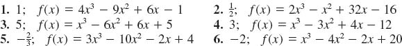
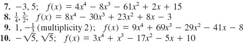
In Problems 7-10, verify that each of the indicated numbers are zeros of the given polynomial function f. Find all other zeros and then give the complete factorization of f(x).
In Problems 11-16, use synthetic division to determine whether the indicated linear polynomial is a factor of the given polynomial function f. If yes, find all other zeros and then give the complete factorization of f (x).

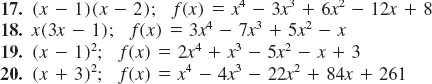
In Problems 17-20, use division to show that the indicated polynomial is a factor of the given polynomial function f. Find all other zeros and then give the complete factorization of f(x).
In Problems 21-26, verify that the indicated complex number is a zero of the given polynomial function f. Proceed as in Example 7 to find all other zeros and then give the complete factorization of f(x).

In Problems 27-32, find a polynomial function f with real coefficients of the indicated degree that possesses the given zeros.
In Problems 33-36, find the zeros of the given polynomial function f. State the multiplicity of each zero.
33. f(x) = x(4x - 5)2(2x - 1)3
34. f(x) = x4 + 6x3 + 9x2
35. f(x) = (9x2 - 4)2
36. f(x) = (x2 + 25)(x2 - 5x + 4)2
In Problems 37 and 38, find the value(s) of k such that the indicated number is a zero of f(x). Then give the complete factorization of f(x).
37. 3; f(x) = 2x3 - 2x2 + k
38. 1; f(x) = x3 + 5x2 - k2x + k
In Problems 39 and 40, find a polynomial function f of the indicated degree whose graph is given in the figure.
39. degree 3

FIGURE 5.3.1 Graph for Problem 39
40. degree 5
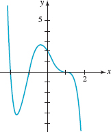
FIGURE 5.3.2 Graph for Problem 40
For Discussion
41. Discuss:
(a) For what positive integer values of n is x - 1 a factor of f(x) = xn - 1?
(b) For what positive integer values of n is x + 1 a factor of f(x) = xn + 1?
Suppose f is a polynomial function of degree 3 with real coefficients. Why can't f(x) have three complex zeros? Put another way, why must at least one zero of a cubic polynomial function be a real number? Can you generalize this result?
What is the smallest degree that a polynomial function f with real coefficients can have such that 1 + i is a complex zero of multiplicity 2? Of multiplicity 3?
Let z = a + bi. Show that ![]() and
and ![]() are real numbers.
are real numbers.
Let z = a + bi. Use the results of Problem 44 to show that
![]()
is a polynomial function with real coefficients.
Try to prove or disprove the following proposition.
Iff is an odd polynomial function, then the graph off passes through the origin
5.4 Real Zeros of Polynomial Functions
![]() Introduction In the preceding section we saw, as a consequence of the Fundamental Theorem of Algebra, that a polynomial function f of degree n has n zeros when the multiplicities of the zeros are counted. We saw too that a zero of a polynomial function could be either a real or a complex number. In this section we confine our attention to real zeros of polynomial functions with real coefficients.
Introduction In the preceding section we saw, as a consequence of the Fundamental Theorem of Algebra, that a polynomial function f of degree n has n zeros when the multiplicities of the zeros are counted. We saw too that a zero of a polynomial function could be either a real or a complex number. In this section we confine our attention to real zeros of polynomial functions with real coefficients.
![]() Real Zeros If a polynomial function f of degree n > 0 has m (not necessarily distinct) real zeros c1, c2,…, cm, then by the Factor Theorem each of the linear polynomials x – c1, x – c2,…, x – cm are factors of f(x). That is,
Real Zeros If a polynomial function f of degree n > 0 has m (not necessarily distinct) real zeros c1, c2,…, cm, then by the Factor Theorem each of the linear polynomials x – c1, x – c2,…, x – cm are factors of f(x). That is,
![]()
where q(x) is a polynomial. Thus n, the degree of f, must be greater than or possibly equal to m, (m ≤ n), the number of real zeros when each is counted according to its multiplicity. Using slightly different words, we restate the last sentence.
Let's summarize some facts about real zeros of a polynomial function f of degree n:
![]() f may not have any real zeros
f may not have any real zeros
For example, the quartic or fourth-degree polynomial function f(x) = x4 + 9 has no real zeros since there exists no real number x satisfying x4 + 9 = 0 or x4 =–9:
![]() f may have m real zeros where m < n
f may have m real zeros where m < n
For example, the third-degree polynomial function f(x) = (x – 1)(x2 + 1) has one real zero:
![]() f may have n real zeros
f may have n real zeros
For example, by factoring the third-degree polynomial function f(x) = x3 - x as f (x) = x(x2 - 1) = x(x + 1)(x - 1) we see that it has three real zeros:
![]() f has at least one real zero when the degree n is odd
f has at least one real zero when the degree n is odd
The last property is a consequence of the fact that complex zeros of a polynomial function f with real coefficients must appear in conjugate pairs and so f cannot have an odd number of complex zeros. Thus if we write down an arbitrary cubic polynomial function such as f(x) = x3 + x + 1, we know that f cannot have just one complex zero nor can it have three complex zeros. Put another way, f(x) = x3 + x + 1 either has exactly one real zero or it has exactly three real zeros. You may have to think about the following property:
![]() If the coefficients of f(x) are positive and the constant term a0 ≠ 0, then any real zeros off must be negative
If the coefficients of f(x) are positive and the constant term a0 ≠ 0, then any real zeros off must be negative
![]() Finding Real Zeros It is one thing to talk about the existence of real and complex zeros of a polynomial function; it is an entirely different problem to actually find these zeros. As pointed out in the chapter introduction, the problem of finding a formula that expresses the zeros of a general n th degree polynomial function f in terms of its coefficients perplexed mathematicians for centuries. We have seen in Sections 1.3 and 3.3 that in the case of a second-degree, or quadratic, polynomial function f(x) = ax2 + bx + c, where the coefficients a, b, and c are real numbers, the zeros c1 and c2 of f can be found using the quadratic formula. The problem of finding zeros of third-degree, or cubic, polynomial functions was solved in the sixteenth century by the Italian mathematicianNiccolÒ Fontana (1499-1557), also known as Tartaglia—”the stammerer.” Around 1540 another Italian mathematician,Lodovico Ferrari(1522-1565) discovered an algebraic formula for determining the zeros for fourth- degree, or quartic, polynomial functions. Since these formulas are complicated and difficult to use, they are seldom discussed in elementary courses. Then in 1824, at age 22, the Norwegian mathematician Niels Henrik Abel (1802-1829), proved it was impossible to find such formulas for the zeros of all general polynomials of degrees n ≥ 5 in terms of their coefficients.
Finding Real Zeros It is one thing to talk about the existence of real and complex zeros of a polynomial function; it is an entirely different problem to actually find these zeros. As pointed out in the chapter introduction, the problem of finding a formula that expresses the zeros of a general n th degree polynomial function f in terms of its coefficients perplexed mathematicians for centuries. We have seen in Sections 1.3 and 3.3 that in the case of a second-degree, or quadratic, polynomial function f(x) = ax2 + bx + c, where the coefficients a, b, and c are real numbers, the zeros c1 and c2 of f can be found using the quadratic formula. The problem of finding zeros of third-degree, or cubic, polynomial functions was solved in the sixteenth century by the Italian mathematicianNiccolÒ Fontana (1499-1557), also known as Tartaglia—”the stammerer.” Around 1540 another Italian mathematician,Lodovico Ferrari(1522-1565) discovered an algebraic formula for determining the zeros for fourth- degree, or quartic, polynomial functions. Since these formulas are complicated and difficult to use, they are seldom discussed in elementary courses. Then in 1824, at age 22, the Norwegian mathematician Niels Henrik Abel (1802-1829), proved it was impossible to find such formulas for the zeros of all general polynomials of degrees n ≥ 5 in terms of their coefficients.

Niels Henrik Abel
![]() Rational Zeros Real zeros of a polynomial function are either rational or irrational numbers. A rational number is a number of the form p/s, where p and s are integers and s ≠ 0. An irrational number is one that is not rational. For example, ¼ and -9 are rational numbers, but
Rational Zeros Real zeros of a polynomial function are either rational or irrational numbers. A rational number is a number of the form p/s, where p and s are integers and s ≠ 0. An irrational number is one that is not rational. For example, ¼ and -9 are rational numbers, but ![]() and π are irrational; that is, neither
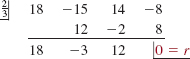
and π are irrational; that is, neither ![]() nor π can be written as a fraction p/s where p and s are integers. So how do we find real zeros for polynomial functions of degree n > 2? First, the bad news: For an irrational real zero, we may have to be content to use an accurate graph to “eyeball” its location on the x-axis, or use an equation solver of a calculator or one of the many sophisticated analytical methods developed over the years to approximate the zero. Now, the good news: We can always find the rational real zeros of any polynomial function with rational coefficients. We have already seen that synthetic division is a useful method for determining whether a given number c is a zero of a polynomial function f(x). When the remainder in the division of f(x) by x - c is r = 0, we have found a zero of the polynomial function f, since r = f(c) = 0. For example,
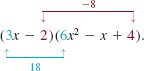
nor π can be written as a fraction p/s where p and s are integers. So how do we find real zeros for polynomial functions of degree n > 2? First, the bad news: For an irrational real zero, we may have to be content to use an accurate graph to “eyeball” its location on the x-axis, or use an equation solver of a calculator or one of the many sophisticated analytical methods developed over the years to approximate the zero. Now, the good news: We can always find the rational real zeros of any polynomial function with rational coefficients. We have already seen that synthetic division is a useful method for determining whether a given number c is a zero of a polynomial function f(x). When the remainder in the division of f(x) by x - c is r = 0, we have found a zero of the polynomial function f, since r = f(c) = 0. For example, ![]() is a zero of f(x) = 18x3 - 15x2 + 14x - 8, since
is a zero of f(x) = 18x3 - 15x2 + 14x - 8, since
Hence by the Factor Theorem, both x - ![]() and the quotient 18x2 - 3x + 12 are factors of f and so we can write the polynomial function as the product
and the quotient 18x2 - 3x + 12 are factors of f and so we can write the polynomial function as the product
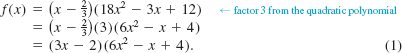
As discussed in the preceding section, if we can factor the polynomial to the point where the remaining factor is a quadratic polynomial, we can then find the remaining two zeros by the quadratic formula. For this example, the factorization in (1) is as far as we can go using real numbers since the zeros of the quadratic factor 6x2 - x + 4 are complex (verify). But the indicated multiplication in (1) illustrates something important about rational zeros. The leading coefficient 18 and the constant term -8 of f(x) are obtained from the products
Thus we see that the denominator 3 of the rational zero ![]() is a factor of the leading coefficient 18 of f(x) = 18x3 - 15x2 + 14x - 8, and the numerator 2 of the rational zero is a factor of the constant term - 8.
is a factor of the leading coefficient 18 of f(x) = 18x3 - 15x2 + 14x - 8, and the numerator 2 of the rational zero is a factor of the constant term - 8.
This example illustrates the following general principle for determining the rational zeros of a polynomial function. Read the following theorem carefully; the coefficients of f are not only real numbers—they must be integers.

The Rational Zeros Theorem deserves to be read several times. Note that the theorem does not assert that a polynomial function f with integer coefficients must have a rational zero; rather, it states that if a polynomial function f with integer coefficients has a rational zero p/s, then necessarily:
![]()
By forming all possible quotients of each integer factor of a0 to each integer factor of an, we can construct a list of potential rational zeros of f.
EXAMPLE 1 Rational Zeros
Find all rational zeros of f(x) = 3x4 - 10x3 - 3x2 + 8x - 2.
Solution We identify the constant terma a0 = - 2 and leading coefficient a4 = 3 and list all the integer factors of a0 and a4 respectively:
![]()
Now we form a list of all possible rational zeros p/s by dividing all the factors of p by ±1and then by ±3:
![]()
We know that the given fourth-degree polynomial function f has four zeros; if any of these zeros is a real number and is rational, then it must appear in the list (2).
To determine which, if any, of the numbers in (2) are zeros, we could use direct substitution into f(x). Synthetic division, however, is usually a more efficient means of evaluating f(x). We begin by testing -1:
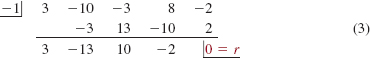
The zero remainder shows r = f(-1) = 0 and so-1 is a zero of f. Hence x -(-1) = x + 1 is a factor of f. Using the quotient found in (3) we can write
![]()
From (4) we see that any other rational zero of f must be a zero of the quotient 3x3 - 13x2 + 10x - 2. Since the latter polynomial is of lower degree, it will be easier to use synthetic division on it rather than on f(x) to check the next rational zero. At this point in the process you should check to see whether the zero just found is a repeated zero. This is done by determining whether the found zero is also a zero of the quotient. A quick check, using synthetic division, shows that -1 is not a repeated zero of f since it is not a zero of 3x3 - 13x2 + 10x - 2. So we move on and determine whether the number 1 is a rational zero of f. Indeed, it is not because the division

shows that the remainder is r = -2 ≠ 0. Checking ![]() , we have
, we have

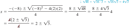
Thus ![]() is a zero. At this point we can stop using synthetic division since (6) indicates that the remaining factor of f is the quadratic polynomial 3x2 - 12x + 6. From the quadratic formula we find that the remaining real zeros are 2 +
is a zero. At this point we can stop using synthetic division since (6) indicates that the remaining factor of f is the quadratic polynomial 3x2 - 12x + 6. From the quadratic formula we find that the remaining real zeros are 2 + ![]() and 2 -
and 2 - ![]() . Therefore the given polynomial functionf has two rational zeros, -1 and
. Therefore the given polynomial functionf has two rational zeros, -1 and ![]() , and two irrational zeros, 2 +
, and two irrational zeros, 2 + ![]() and 2 -
and 2 - ![]() .
.
If you have access to technology, your selection of rational numbers to test in Example 1 can be motivated by a graph of the function f(x) = 3x4 - 10x3 - 3x2 + 8x - 2. With the aid of a graphing utility we obtain the graphs in FIGURE 5.4.1. In Figure 5.4.1(a) it would appear that f has at least three real zeros. But by “zooming in” on the graph on the interval [0, 1], Figure 5.4.1(b) reveals that f actually has four real zeros: one negative and three positive. Thus, once you have determined one negative rational zero of f you may disregard all other negative numbers as potential zeros.
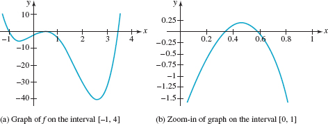
FIGURE 5.4.1 Graph of function f in Example 1
EXAMPLE 2 Complete Linear Factorization
Since the function f in Example 1 is of degree 4 and we have found four real zeros we can give its complete factorization. Using the leading coefficient a4 = 3, it follows from (6) of Section 4.3 that
![]()
EXAMPLE 3 Rational Zeros
Find all rational zeros of f(x) = x4 + 4x3 + 5x2 + 4x + 4.
Solution In this case the constant term is a0 = 4 and the leading coefficient is a4 = 1. The integer factors of a0 and a4 are, respectively:
![]()
The list of all possible rational zeros p/s is
![]()
Since all the coefficients of f are positive, substituting a positive number from the foregoing list into f(x) can never result in f(x) = 0. Thus the only numbers that are potential rational zeros are -1, -2, and -4. From the synthetic division
we see that -1 is not a zero. However, from

we see that -2 is a zero. We now test to see whether -2 is a repeated zero. Using the coefficients in the quotient,
it follows that - 2 is a zero of multiplicity 2. So far we have shown that
![]()
Since the zeros of x2 + 1 are the complex conjugates i and -i, we can conclude that - 2 is the only real rational zero of f(x).
EXAMPLE 4 No Rational Zeros
Consider the polynomial function f(x) = x5 - 4x - 1.The only possible rational zeros are -1 and 1, and it is easy to see that neither f(-1) nor f (1) are 0. Thus f has no rational zeros. Since f is of odd degree we know that it has at least one real zero and so that zero must be an irrational number. With the aid of a graphing utility we obtain the graph in FIGURE 5.4.2. Note in the figure, the graph to the right of x = 2 cannot turn back down and the graph to the left of x = -2 cannot turn back up so that graph crosses the x-axis five times since that shape of the graph would be inconsistent with the end behavior of f. Thus we can conclude that the function f possesses three irrational real zeros and two complex conjugate zeros. The best we can do here is to approximate these zeros. Using a computer algebra system such as Mathematica we can approximate both the real and the complex zeros. We find these approximations to be -1.34, -0.25,1.47, 0.061 + 1.42i, and 0.061 - 1.42i.
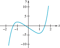
FIGURE 5.4.2 Graph of f in Example 4
Although the Rational Zeros Theorem requires that the coefficients of a polynomial function f be integers, in some circumstances we can apply the theorem to a polynomial function with some rational noninteger coefficients. The next example illustrates the concept.
EXAMPLE 5 Noninteger Coefficients
Find the rational zeros of ![]()
Solution By multiplying f by the least common denominator 12 of all the rational coefficients we obtain a new function g with integer coefficients:
![]()
In other words, g(x) = 12 f(x). If c is a zero of the function g, then c is also zero of f because g(c) = 12f(c) = 0 implies f(c) = 0. After working through the numbers in the list of potential rational zeros
![]()
we find that -1/5 and ![]() are zeros of g, and hence are zeros of f.
are zeros of g, and hence are zeros of f.

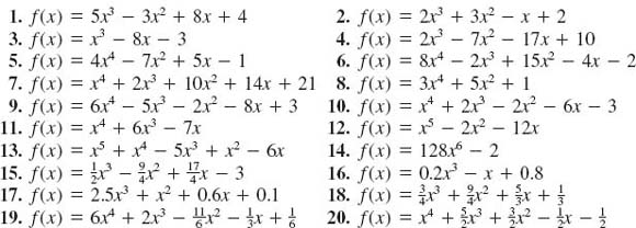
In Problems 1-20, find all rational zeros of the given polynomial function f.
In Problems 21-30, find all real zeros of the given polynomial function f. Then factor f(x) using only real numbers.
In Problems 31-36, find all real solutions of the given equation.
In Problems 37 and 38, find a polynomial function f of the indicated degree with integer coefficients that possesses the given rational zeros.
37. degree 4; -4, ![]() , 1, 3
, 1, 3
38. degree 5; -2, -![]() , ½, 1 (multiplicity two)
, ½, 1 (multiplicity two)
In Problems 39 and 40, find a cubic polynomial function f that satisfies the given conditions.
39. rational zeros 1 and 2, f(0) = 1 and f (-1) = 4
40. rational zero ½, irrational zeros 1 + ![]() and 1 -
and 1 - ![]() , coefficient of x is 2
, coefficient of x is 2
Miscellaneous Applications
Construction of a Box A box with no top is made from a square piece of cardboard by cutting square pieces from each corner and then folding up the sides. See FIGURE 5.4.3. The length of one side of the cardboard is 10 inches. Find the length of one side of the squares that were cut from the corners if the volume of the box is 48 in3.

FIGURE 5.4.3 Box in Problem 41
Deflection of a Beam A cantilever beam 20 ft long with a load of 600 lb at its right end is deflected by an amount ![]() , where d is measured in inches and x in feet. See FIGURE 5.4.4. Find x when the deflection is 0.1215 in. When the deflection is 1 in.
, where d is measured in inches and x in feet. See FIGURE 5.4.4. Find x when the deflection is 0.1215 in. When the deflection is 1 in.
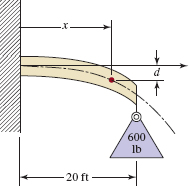
FIRURE 5.4.4 Cantilever beam in Problem 42
For Discussion
Discuss: What is the maximum number of times the graphs of the polynomial functions
![]()
can intersect?
Consider the polynomial function ![]() , where the coefficients a n-1…, a1, a0 are nonzero even integers. Discuss why -1 and 1 cannot be zeros of f(x).
, where the coefficients a n-1…, a1, a0 are nonzero even integers. Discuss why -1 and 1 cannot be zeros of f(x).
A polynomial function is a continuous function; that is, the graph of a polynomial function has no breaks in it. If f(x) = 4x3 - 11x2 + 14x - 6, show that f (0) f(1) < 0. Explain why this shows that f(x) has a zero in the interval [0, 1]. Find the zero.
If the leading coefficient of a polynomial function with integer coefficients is 1, what can be said about the possible rational zeros?
If k is a prime number **such that k > 2, what are the possible rational zeros of
![]()
Show that ![]() is a zero of the polynomial function f(x) = x3 - 7. Explain why this proves that
is a zero of the polynomial function f(x) = x3 - 7. Explain why this proves that ![]() is an irrational number.
is an irrational number.
5.5 Approximating Real Zeros
![]() Introduction A polynomial function f is a continuous function. Recall from Section 3.4, this means that the graph of y = f(x) has no breaks, gaps, or holes in it. The following result is a direct consequence of continuity.
Introduction A polynomial function f is a continuous function. Recall from Section 3.4, this means that the graph of y = f(x) has no breaks, gaps, or holes in it. The following result is a direct consequence of continuity.
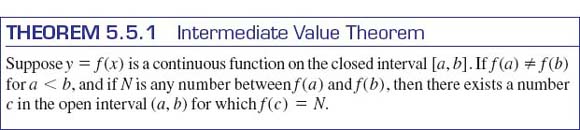
As we see in FIGURE 5.5.1, the Intermediate Value Theorem simply states that a continuous function f(x) takes on all values between the numbers f(a) and f(b). In particular, if the function values f(a) and f(b) have opposite signs, then by identifying N = 0, we can say that there is at least one number in the open interval (a, b) for which f(c) = 0. In other words,

FIGURE 5.5.1 f(x) takes on all values between f(a) and f(b)
![]()
The plausibility of this conclusion is illustrated in FIGURE 5.5.2

FIGURE 5.5.2 Locating zeros using the Intermediate Value Theorem
EXAMPLE 1 Using the Intermediate Value Theorem
Consider the polynomial function f(x) = x3 – 3x – 1. From the data in the accompanying table we conclude from (1) that f has a real zero in each of the intervals [-2, -1], [-1, 0], and [1, 2]. But using Theorem 5.4.2, we can verify that f has no rational zeros and so the three real zeros of f are irrational numbers. As seen in FIGURE 5.5.3 the graph of f crosses the line y = 0 (the x-axis) 3 times.

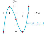
FIGURE 5.5.3 Graph of function in Example 1
In the next example we will obtain an approximation to one of the irrational zeros in Example 1 using a technique called the bisection method.
![]() Bisection Method The basic idea of this method starts with the assumption that a function f is continuous and f(a) and f(b) have opposite signs. From this we know that there exists a number c in (a, b) for which f(c) = 0. Then the midpoint m = (a + b)/2 of the interval [a, b] is an approximation to c. If m = (a + b)/2 is not a zero off, then there is a zero c in an interval (either the open interval (a, m) or the open interval (m, b)) that is one-half the length of the original interval [a, b]. If, say, c lies in (m, b) as shown in FIGURE 5.5.4, we then divide this shorter interval in half: Either the new midpoint is a zero or the zero c lies in an interval that is one-fourth the length of the interval [a, b]. Continuing in this manner, we can locate the zero c of f in successively shorter intervals. We will then take the midpoints of these intervals as approximations to the zero c. Using this method, we see in FIGURE 5.5.4 that the error in an approximation to a zero in an interval is less than one-half the length of the interval.
Bisection Method The basic idea of this method starts with the assumption that a function f is continuous and f(a) and f(b) have opposite signs. From this we know that there exists a number c in (a, b) for which f(c) = 0. Then the midpoint m = (a + b)/2 of the interval [a, b] is an approximation to c. If m = (a + b)/2 is not a zero off, then there is a zero c in an interval (either the open interval (a, m) or the open interval (m, b)) that is one-half the length of the original interval [a, b]. If, say, c lies in (m, b) as shown in FIGURE 5.5.4, we then divide this shorter interval in half: Either the new midpoint is a zero or the zero c lies in an interval that is one-fourth the length of the interval [a, b]. Continuing in this manner, we can locate the zero c of f in successively shorter intervals. We will then take the midpoints of these intervals as approximations to the zero c. Using this method, we see in FIGURE 5.5.4 that the error in an approximation to a zero in an interval is less than one-half the length of the interval.
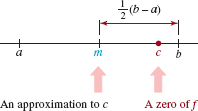
FIGURE 5.5.4 If f(a) and f(b) have opposite signs, then a zero c of f must lie either in [a, m] or in [m, b]
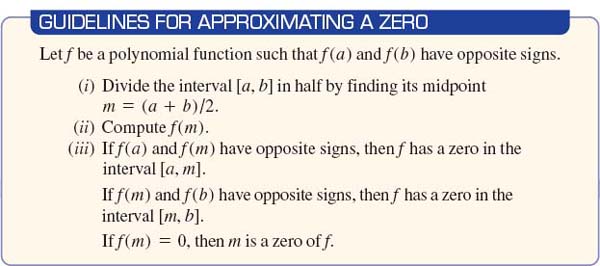
We summarize the discussion as follows:
EXAMPLE 2 Using the Bisection Method
Find an approximation to the zero of f(x) = x3 – 3x – 1 in the interval [1, 2] that is accurate to three decimal places.
Solution Recall from Example 1 that f(1) < 0 and f(2) > 0. Now to obtain the desired accuracy, we must have the error less than 0.0005.*** The first approximation to the zero in [1, 2] is
![]()
Since f(1.5) = -2.15 > 0, the zero lies in [1.5, 2].
The second approximation to the zero is
![]()
Since f(1.75) = -0.89065 > 0, the zero lies in [1.75, 2].
The third approximation to the zero is
![]()
Continuing in this manner we eventually find
![]()
Thus the number1.879 is an approximation to the zero of f in [1, 2] that is accurate to three decimal places.
In Example 2 we leave the approximation to the zeros of f(x) = x3 - 3x - 1 in zeros in [a, b] the intervals [-2, -1] and [-1, 0] as exercises.
If f(a) and f(b) have the same sign, the polynomial function f could still have one or more zeros in the interval [a, b]. See FIGURE 5.5.5
![]() Note of Caution
Note of Caution
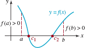
FIGURE 5.5.5 f(a) and f(b) are positive, yet there are two zeros in [a, b]

In Problems 1 and 2, find an approximation that is accurate to three decimal places to the zero of f(x) = x3 - 3x - 1 in the given interval.
[-2, -1]
[-1, 0]
In Problems 3-6, use the bisection method to approximate to an accuracy of three decimal places the zero(s) indicated by the graph of the given function.
f(x) = x3 - x2 + 4
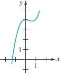
FIGURE 5.5.6Graph for Problem 3
f(x) = x3 - x + 11
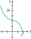
FIGURE 5.5.7Graph for Problem 4
f(x) = x4 - 4x3 + 10

FIGURE 5.5.8 Graph for Problem 5
f(x) = 3x5 - 5x3 + 1
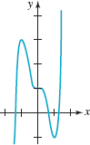
FIGURE 5.5.9 Graph for Problem 6
In Problems 7 and 8, use the bisection method to approximate to an accuracy of three decimal places the x-coordinates of the point(s) of intersection of the given graphs.
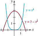
FIGURE 5.5.10 Graph for Problem 7
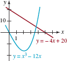
FIGURE 5.5.11 Graph for Problem 8
Miscellaneous Applications
Sinking Wooden Ball A spherical wooden ball of radius r is placed in water. To determine the depth h to which the ball will sink, we equate the weight of the displaced water with the weight of the ball (Archimedes' principle):
![]()
where ρw and ρb are the densities of water and wood, respectively. See FIGURE 5.5.12. Suppose ρb = 0.4 ρw and r = 2 in. Use the bisection method to approximate to an accuracy of two decimal places the depth h to which a wooden ball will sink.
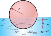
FIGURE 5.5.12 Floating ball in Problem 9
Sag of a Cable The length L of a cable between two vertical supports of a suspension bridge is given by
![]()
where r is the span of the supports and s is the sag of the cable between the supports. See FIGURE 5.5.13. If r = 400 ft and L = 404 ft, use the bisection method to approximate the sag s of the cable to an accuracy of two decimal places. [Hint: Consider the interval [20, 30].]

FIGURE 5.5.13 Suspension bridge in Problem 10
5.6 Rational Functions
![]() Introduction Many functions are built up out of polynomial functions by means of arithmetic operations and function composition (see Section 4.5). In this section we construct a class of functions by forming the quotient of two polynomial functions.
Introduction Many functions are built up out of polynomial functions by means of arithmetic operations and function composition (see Section 4.5). In this section we construct a class of functions by forming the quotient of two polynomial functions.
As rational numbers are built out of integers, so too a rational function is built out of polynomial functions.
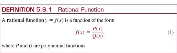
For example, the following three functions are rational functions:

The function
![]()
is not a rational function. In (1) we cannot allow the denominator to be zero. So the domain of a rational function f(x) = P(x)/Q(x) is the set of all real numbers except those numbers for which the denominator Q(x) is zero. For example, the domain of the rational function f(x) = (2x3 – 1)/(x2 – 9) is {x | x ≠ –3, x ≠ 3} or (– ∞, – 3) ∪ (–3, 3) ∪ (3, ∞).It goes without saying that we also disallow the zero polynomial Q(x) = 0 as a denominator.
![]() Graphs Graphing a rational function f is a little more complicated than graphing a polynomial function because in addition to paying attention to
Graphs Graphing a rational function f is a little more complicated than graphing a polynomial function because in addition to paying attention to
![]() intercepts,
intercepts,
![]() symmetry, and
symmetry, and
![]() shifting/reflecting/stretching of known graphs, you should also keep an eye on the domain of f, and
shifting/reflecting/stretching of known graphs, you should also keep an eye on the domain of f, and
![]() the degrees of P(x) and Q(x).
the degrees of P(x) and Q(x).
The latter two topics are important in determining whether a graph of a rational function possesses asymptotes.
The y-intercept is the point (0, f(0)), provided the number 0 is in the domain of f. For example, the graph of the rational function f(x) = (1 – x)/x does not cross the y-axis since f(0) is not defined. If the polynomials P(x) and Q(x) have no common factors, then the x-intercepts of the graph of the rational function f(x) = P(x)/Q(x) are the points whose x-coordinates are the real zeros of the numerator P(x). In other words, the only way we can have f(x) = P(x)/Q(x) = 0 is to have P(x) = 0. The graph of a rational functionf is symmetric with respect to the y-axis if f(–x) = -f(x), and symmetric with respect to the origin if f(–x) = –f(x). Since it is easy to spot an even or an odd polynomial function (see page 230), here is an easy way to determine symmetry of the graph of a rational function. We again assume that P(x) and Q(x) have no common factors.
![]() The quotient of two even functions is even. (2)
The quotient of two even functions is even. (2)
![]() The quotient of two odd functions is even. (3)
The quotient of two odd functions is even. (3)
![]() The quotient of an even and an odd function is odd. (4)
The quotient of an even and an odd function is odd. (4)
See Problem 48 in Exercises 5.6.
We have already seen the graphs of two simple rational functions, y = 1/x and y = 1/x2 in Figures 4.2.1(e) and 4.2.1(f). You are encouraged to review those graphs at this time. Note that P(x) = 1 is an even function and Q(x) = x is an odd function, so y = 1/x is an odd function by (4). On the other hand, P(x) = 1 is an even function and Q(x) = x2 is an even function, so y = 1/x2 is an even function by (2).
EXAMPLE 1 Shifted Reciprocal Function
Graph of function ![]()
Solution The graph possesses no symmetry since Q(x) = x -1 is neither even nor odd. Since f(0) = -2, the y-intercept is (0, 22). Because P(x) = 2 is never 0, there are no x-intercepts. You might also recognize that the graph of this rational function is the graph of the reciprocal function y = 1/x stretched vertically by a factor of 2 and shifted 1 unit to the right. The point (1, 1) is on the graph of y = 1/x; in FIGURE 5.6.1, after the vertical stretch and horizontal shift, the corresponding point on the graph of y = 2/(x - 1) is (2, 2).
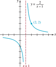
FIGURE 5.6.1 Graph of function in Example 1
The vertical line x = 1 and the horizontal line y = 0 (the equation of the x-axis) are of special importance for this graph.
The vertical dashed line x = 1 in FIGURE 5.6.1 is the y-axis in Figure 4.2.1(e) shifted 1 unit to the right. Although the number 1 is not in the domain of the given function, we can evaluate f at values of x that are near 1. For example, you should verify that

The table in (5) shows that for values of x close to 1 the corresponding function values f(x) are large in absolute value. On the other hand, for values of x for which |x| is large, the corresponding function values f(x) are near 0. For example, you should verify that
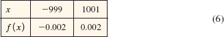
Geometrically, as x approaches 1, the graph of the function approaches the vertical line x = 1, and as |x| increases without bound the graph of the function approaches the horizontal line y = 0.
![]() Notation To indicate that x is approaching a number a, we use the notation
Notation To indicate that x is approaching a number a, we use the notation
![]() x → a- to mean that x is approaching a from the left, that is, through numbers that are less than a,
x → a- to mean that x is approaching a from the left, that is, through numbers that are less than a,
![]() x → a+ to mean that x is approaching a from the right, that is, through numbers that are greater than a, and
x → a+ to mean that x is approaching a from the right, that is, through numbers that are greater than a, and
![]() x → a to mean that x is approaching a from both the left and the right.
x → a to mean that x is approaching a from both the left and the right.
We also use the infinity symbols and the notation
![]() x → – ∞ to mean that x becomes unbounded in the negative direction, and
x → – ∞ to mean that x becomes unbounded in the negative direction, and
![]() x → ∞ to mean that x becomes unbounded in the positive direction.
x → ∞ to mean that x becomes unbounded in the positive direction.
![]() This notation was used in the discussion of end behavior in Section 5.1.
This notation was used in the discussion of end behavior in Section 5.1.
Similar interpretations are given to the symbols f(x) → –∞ and f(x) → ∞. These notational devices are a convenient way of describing the behavior of a function either near a number x = a or as x increases to the right or decreases to the left. Thus, in Example 1 it is apparent from (5) and FIGURE 5.6.1 that
![]()
In words, the notation in the preceding line signifies that the function values are decreasing without bound as x approaches 1 from the left, and the function values are increasing without bound as x approaches 1 from the right. From (6) and FIGURE 5.6.1 it should also be apparent that
![]()
![]() Asymptotes In FIGURE 5.6.1, the vertical line whose equation is x = 1 is called a vertical asymptote for the graph off, and the horizontal line whose equation is y = 0 is called a horizontal asymptote for the graph of f.
Asymptotes In FIGURE 5.6.1, the vertical line whose equation is x = 1 is called a vertical asymptote for the graph off, and the horizontal line whose equation is y = 0 is called a horizontal asymptote for the graph of f.
In this section we will examine three types of asymptotes that correspond to the three types of lines studied in Section 3.3: vertical lines, horizontal lines, and slant (or oblique) lines. The characteristic of any asymptote is that the graph of a function f must get close to, or approach, the line.

FIGURE 5.6.2 illustrates four of the six possibilities listed in (7) for the unbounded behavior of a function f near a vertical asymptote x = a. If the function exhibits the same kind of unbounded behavior from both sides of x = a, then we write
![]()
or
![]()
In Figure 5.6.2(d) we see that f(x) → ∞ as x → a– and f(x) → ∞ as x → a+, and so we write f(x) → ∞ as x → a.
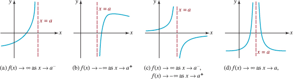
FIGURE 5.6.2 The line x = a is a vertical asymptote
If x = a is a vertical asymptote for the graph of a rational function f(x) = P(x)/Q(x), then the function values f(x) become unbounded as x approaches a from both sides, that is, from the right (x → a+) and from the left (x → a-). The graphs in Figures 5.6.2(c) and 5.6.2(d) (or the reflection of these graphs in the x-axis) are typical graphs of a rational function with a single vertical asymptote. As can be seen from these figures, a rational function with a vertical asymptote is a discontinuous function. There is an infinite break in each graph at x = a. As seen in Figures 5.6.2(c) and 5.6.2(d) a single vertical asymptote divides the xy-plane into two regions; within each region there is a single piece or branch of the graph of the rational function f.
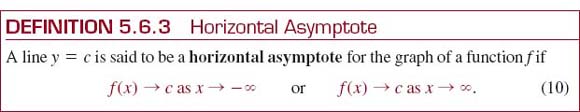
In FIGURE 5.6.3 we have illustrated some typical horizontal asymptotes. We note, in conjunction with Figure 5.6.3(d) that, in general, the graph of a function can have at most two horizontal asymptotes but the graph of a rational function f(x) = P(x) / Q(x) can have at most one. If the graph of a rational function f possesses a horizontal asymptote y = c, then as shown in Figure 5.6.3(c),
Remember this.![]()
![]()
The last line is a mathematical description of the end behavior of the graph of a rational function with a horizontal asymptote. Also, the graph of a function can never cross a vertical asymptote but, as suggested in Figure 5.6.3(a), a graph can cross a horizontal asymptote.

FIGURE 5.6.3 The line y = c is a horizontal asymptote
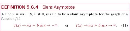
![]() A slant asymptote is also called an oblique asymptote.
A slant asymptote is also called an oblique asymptote.
The notation in (11) means that the graph of f possesses a slant asymptote whenever the function values f(x) become closer and closer to the values of y on the line y = mx + b as x becomes large in absolute value. Another way of stating (11) is: A line y = mx + b is a slant asymptote for the graph of f if the vertical distance d(x) between points with the same x-coordinate on the two graphs satisfies
![]()
See FIGURE 5.6.4. We note that if a graph of a rational function f(x) = P(x)/Q(x) possesses a slant asymptote it can have vertical asymptotes, but the graph cannot have a horizontal asymptote.
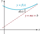
FIGURE 5.6.4Slant asymptote is y = mx + b
On a practical level, vertical and horizontal asymptotes of the graph of a rational function f can be determined by inspection. So for the sake of discussion let us suppose that
![]()
represents a general rational function.
![]() Finding Vertical Asymptotes Let us assume that the polynomial functions P(x) and Q(x) in (12) have no common factors. In that case:
Finding Vertical Asymptotes Let us assume that the polynomial functions P(x) and Q(x) in (12) have no common factors. In that case:
 If a is a real number such that Q(a) = 0, then the line x = a is a vertical asymptote for the graph of f.
Since Q(x) is a polynomial function of degree m, it can have up to m real zeros, and so the graph of a rational function f can have up to m vertical asymptotes. If the graph of a rational functionf has, say, k (k ≤ m) vertical asymptotes, then the k vertical lines divide the xy-plane into k + 1 regions. Thus the graph of this rational function would have k + 1 branches.
EXAMPLE 2 Vertical Asymptotes
(a) Inspection of the rational function ![]() shows that the denominator Q(x) = x2 - 4 = (x + 2)(x - 2) = 0 at x = -2 and x = 2. These are equations of vertical asymptotes for the graph of f. The graph of f has three branches: one to the left of the line x = -2, one between the lines x = -2 and x = 2, and one to the right of the line x = 2.
shows that the denominator Q(x) = x2 - 4 = (x + 2)(x - 2) = 0 at x = -2 and x = 2. These are equations of vertical asymptotes for the graph of f. The graph of f has three branches: one to the left of the line x = -2, one between the lines x = -2 and x = 2, and one to the right of the line x = 2.
(b) The graph of the rational function ![]() has no vertical asymptotes since Q(x) = x2 + x + 4 ≠ 0 for all real numbers.
has no vertical asymptotes since Q(x) = x2 + x + 4 ≠ 0 for all real numbers.
![]() Finding Horizontal Asymptotes When we discussed end behavior of a polynomial function P(x) of degree n, we pointed out that P(x) behaves like y = an xn, that is, P(x) ≈ an xn, for values of x large in absolute value. As a consequence, we see from
Finding Horizontal Asymptotes When we discussed end behavior of a polynomial function P(x) of degree n, we pointed out that P(x) behaves like y = an xn, that is, P(x) ≈ an xn, for values of x large in absolute value. As a consequence, we see from

that f(x) behaves like ![]() Therefore:
Therefore:

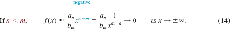
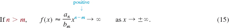
From (13), (14), and (15) we glean the following three facts about horizontal asymptotes for the graph of f(x) = P(x)/Q(x).
![]()
![]()
![]()
EXAMPLE 3 Horizontal Asymptotes
Determine whether the graph of each of the following rational functions possesses a horizontal asymptote.
![]()
Solution (a) Since the degree of the numerator 3x2 + 4x - 1 is the same as the degree of the denominator 8x2 + x (both degrees are 2) we see from (13) that
![]()
As summarized in (16), y = 3/8 is a horizontal asymptote for the graph of f.
(b) Since the degree of the numerator 4x3 + 7x + 8 is 3 and the degree of the denominator 2x4 + 3x2 - x + 6 is 4 (and 3 < 4) we see from (14) that
![]()
As summarized in (17), y = 0 (the x-axis) is a horizontal asymptote for the graph of f.
(c) Since the degree of the numerator 5x3 + x2 – 1 is 3 and the degree of the denominator 2x + 3 is 1 (and 3 > 1) we see from (15) that
![]()
As summarized in (18), the graph of f has no horizontal asymptote.
In the graphing examples that follow we will assume that P(x) and Q(x) in (12) have no common factors.
EXAMPLE 4 Graph of a Rational Function
Graph the function ![]() .
.
Solution Here are some things we look at to sketch the graph of f.
Symmetry: No symmetry. P(x) = 3 – x and Q(x) = x + 2 are neither even nor odd.
Intercepts:f(0) = ![]() and so the y-intercept is (0,
and so the y-intercept is (0, ![]() ). Setting P(x) = 0 or 3 – x = 0 implies 3 is a zero of P. The single x-intercept is (3, 0).
). Setting P(x) = 0 or 3 – x = 0 implies 3 is a zero of P. The single x-intercept is (3, 0).
Vertical Asymptotes: Setting Q(x) = 0 or x + 2 = 0 gives x = –2. The line x = –2 is a vertical asymptote.
Branches: Because there is only a single vertical asymptote, the graph of f consists of two distinct branches, one to the left of x = –2 and one to the right of x = –2.
Horizontal Asymptote:The degree of P and the degree of Q are the same (namely, 1) and so the graph of f has a horizontal asymptote. By rewriting f as ![]() we see that the ratio of leading coefficients is –1/1 = –1.
we see that the ratio of leading coefficients is –1/1 = –1.
From (16) we see that the line y = –1 is a horizontal asymptote.
The Graph: We draw the vertical and horizontal asymptotes using red dashed lines. The right branch of the graph of f is drawn through the intercepts (0, ![]() ) and (3, 0) in such a manner that it approaches both asymptotes. The left branch is drawn below the horizontal asymptote y = –1. Were we to draw this branch above the horizontal asymptote it would have to be near the horizontal asymptote from above and near the vertical asymptote from the left. In order to do this the branch of the graph would have to cross the x-axis, but since there are no more x-intercepts this is impossible. See FIGURE 5.6.5.
) and (3, 0) in such a manner that it approaches both asymptotes. The left branch is drawn below the horizontal asymptote y = –1. Were we to draw this branch above the horizontal asymptote it would have to be near the horizontal asymptote from above and near the vertical asymptote from the left. In order to do this the branch of the graph would have to cross the x-axis, but since there are no more x-intercepts this is impossible. See FIGURE 5.6.5.
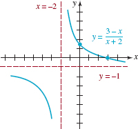
FIGURE 5.6.5 Graph of function in Example 4
EXAMPLE 5 Using Transformations in Example 4
Long division and rigid transformations can sometimes be an aid in graphing rational functions. Note that if we carry out the long division for the function f in Example 4, then we see that
![]()
Thus, starting with the graph of y = 1/x, we stretch it vertically by a factor of 5. Then shift the graph of y = 5/x two units to the left. Finally, shift y = 5/(x + 2) one unit vertically downward. You should verify that the net result is the graph in FIGURE 5.6.5.
EXAMPLE 6 Graph of a Rational Function
Graph the function ![]()
Solution
Symmetry: Since P(x) = x is odd and Q(x) = 1 – x2 is even, the quotient P(x)/Q(x) is odd. The graph of f is symmetric with respect to the origin.
Intercepts: f(0) = 0 and so the y-intercept is (0, 0). Setting P(x) = x = 0 gives x = 0. Thus the only intercept is (0, 0).
Vertical Asymptotes: Setting Q(x) = 0 or 1 – x2 = 0 = 0 gives x = –1 and x = 1.The lines x = –1 and x = 1 are vertical asymptotes.
Branches: Because there are two vertical asymptotes, the graph of f consists of three distinct branches, one to the left of the line x = –1, one between the lines x = –1 and x = 1, and one to the right of the line x = 1.
Horizontal Asymptote: Since the degree of the numerator x is 1 and the degree of the denominator 1 – x2 is 2 (and 1 < 2) it follows from (14) and (17) that y = 0 is a horizontal asymptote for the graph of f.
The Graph: We can plot the graph for x ≥ 0 and then use symmetry to obtain the remaining part of the graph of x < 0. We begin by drawing the vertical asymptotes using dashed lines. The half-branch of the graph of f on the interval [0, 1) is drawn starting at (0, 0). The function f must then increase because P(x) = x > 0 and Q(x) = 1 – x2 > 0 indicates that f(x) > 0 for 0 < x < 1. This implies that near the vertical asymptote x = 1, f(x) → ∞ as x → 1–. The branch of the graph for x > 1 is drawn below the horizontal asymptote y = 0 since P(x) = x > 0 and Q(x) = 1 – x2 < 0 imply f(x) < 0. Thus f(x) → –∞ as x → 1+ and f(x) → 0 as x → ∞. The remainder of the graph for x < 0 is obtained by reflecting the graph for x < 0 through the origin. See FIGURE 5.6.6.
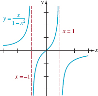
FIGURE 5.6.6 Graph of function in Example 6
EXAMPLE 7 Graph of a Rational Function
Graph the function ![]()
Solution The given function f is similar to the function in Example 6 in that f is an odd function, (0, 0) is the only intercept of its graph, and its graph has the horizontal asymptote. However, note that since 1 + x2 > 0 for all real numbers, there are no vertical asymptotes. Thus there are no branches; the graph is one continuous curve. For x ≥ 0, the graph passes through (0, 0) and then must increase since f(x) > 0 for x > 0. Also, f must attain a relative maximum and then decrease in order to satisfy the condition f(x) → 0 as x → ∞. As mentioned in Section 5.1, the exact location of this relative maximum can be obtained through calculus techniques. Finally, we reflect the portion of the graph for x > 0 through the origin. The graph must look something like that shown in FIGURE 5.6.7.
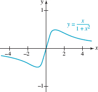
FIGURE 5.6.7 Graph of function in Example 7
![]() Finding Slant Asymptotes Let us again assume that the polynomials P(x) and Q(x) in (11) have no common factors. In that case we can recognize the existence of a slant asymptote in the following manner:
Finding Slant Asymptotes Let us again assume that the polynomials P(x) and Q(x) in (11) have no common factors. In that case we can recognize the existence of a slant asymptote in the following manner:
If the degree of P(x) is precisely one greater than the degree of Q(x), that is, if the degree of Q(x) is m and the degree of P(x) is n = m + 1, then the graph of f possesses a slant asymptote.
We find the slant asymptote by division. Using long division to divide P(x) by Q(x) yields a quotient that is a linear polynomial mx + b and a polynomial remainder R(x):
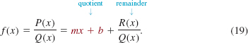
Because the degree of R(x) must be less than the degree of the divisor Q(x), we have R(x)/Q(x) → 0 as x → –∞ and as x → ∞, and consequently
![]()
In other words, an equation of the slant asymptote is y = mx + b, where mx + b is the quotient in (19).
When the denominator Q(x) is a linear polynomial, we can use synthetic division to carry out the long division.
EXAMPLE 8 Graph with a Slant Asymptote
Graph the function ![]()
Solution
Symmetry: No symmetry. P(x) = x2 – x – 6 and Q(x) = x – 5 are neither even nor odd.
Intercepts: f(0) = ![]() and so the y-intercept is (0,
and so the y-intercept is (0, ![]() ). Setting P(x) = 0 or x2 – x – 6 = 0 or (x + 2)(x – 3) = 0 shows that –2 and 3 are zeros of P(x). The x-intercepts are (–2, 0) and (3, 0).
). Setting P(x) = 0 or x2 – x – 6 = 0 or (x + 2)(x – 3) = 0 shows that –2 and 3 are zeros of P(x). The x-intercepts are (–2, 0) and (3, 0).
Vertical Asymptotes: Setting Q(x) = 0 or x – 5 = 0 gives x = 5. The line x = 5 is a vertical asymptote.
Branches: The graph of f consists of two branches, one to the left of x = 5 and one to the right of x = 5.
Horizontal Asymptote: None.
Slant Asymptote: Since the degree of P(x) = x2 – x – 6 (which is 2) is exactly one greater than the degree of Q(x) = x – 5 (which is 1), the graph of f(x) has a slant asymptote. To find it, we divide P(x) by Q(x). Because Q(x) is a linear polynomial we can use synthetic division:
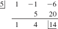
Recall, the latter notation means that
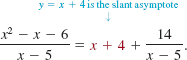
Note again that 14/(x – 5) → 0 as x → ±∞. Hence the line y = x + 4 is a slant asymptote.
The Graph: Using the foregoing information we obtain the graph in FIGURE 5.6.8. The asymptotes are the dashed red lines in the figure.
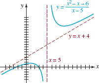
FIGURE 5.6.8 Graph of function in Example 8
EXAMPLE 9 Graph with a Slant Asymptote
By inspection it should be apparent that the graph of the rational function ![]() possesses a slant asymptote but no vertical asymptotes. Since the denominator is a quadratic polynomial we resort to long division to obtain
possesses a slant asymptote but no vertical asymptotes. Since the denominator is a quadratic polynomial we resort to long division to obtain
![]()
The slant asymptote is the line y = x. The graph has no symmetry. The y-intercept is (0, 12). The lack of vertical asymptotes indicates that the function f is continuous; its graph consists of an unbroken curve. Because the numerator is a polynomial of odd degree we know that it has at least one real zero. Since x3 – 8x + 12 = 0 has no rational roots, we can use the approximation method of Section 5.5 or graphical techniques to show that the equation possesses only one real irrational root. Thus the x-intercept is approximately (–3.4, 0). The graph of f is given in FIGURE 5.6.9. Notice in that figure, the graph of f crosses the slant asymptote shown as a red dashed line.
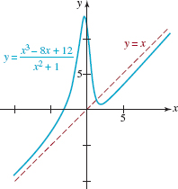
FIGURE 5.6.9 Graph of function in Example 9
![]() Hole in a Graph We assumed throughout the foregoing discussion of asymptotes of rational functions that the polynomial functions P(x) and Q(x) in (1) have no common factors. We now know that if a is a real number such that Q(a) = 0, and P(x) and Q(x) have no common factors, then the line x = a is a vertical asymptote for the graph of f. Because Q is a polynomial function it follows from the Factor Theorem that Q(x) = (x – a)q(x). The assumption that the numerator P and denominator Q have no common factors tells us that x – a is not a factor of P and so P(a) ≠ 0. When P(a) = 0 and Q(a) = 0, then x = a may not be a vertical asymptote. For example, when a is a simple zero of both P and Q, then x = a is not a vertical asymptote for the graph of f(x) = P(x)/Q(x). To see this, we know from the Factor Theorem that if P(a) = 0 and Q(a) = 0 then x – a is a common factor of P and Q and so P(x) = (x – a)p(x) and Q(x) = (x – a)q(x), where p and q are polynomials such that p(a) ≠ 0 and q(a) ≠ 0. After cancelling
Hole in a Graph We assumed throughout the foregoing discussion of asymptotes of rational functions that the polynomial functions P(x) and Q(x) in (1) have no common factors. We now know that if a is a real number such that Q(a) = 0, and P(x) and Q(x) have no common factors, then the line x = a is a vertical asymptote for the graph of f. Because Q is a polynomial function it follows from the Factor Theorem that Q(x) = (x – a)q(x). The assumption that the numerator P and denominator Q have no common factors tells us that x – a is not a factor of P and so P(a) ≠ 0. When P(a) = 0 and Q(a) = 0, then x = a may not be a vertical asymptote. For example, when a is a simple zero of both P and Q, then x = a is not a vertical asymptote for the graph of f(x) = P(x)/Q(x). To see this, we know from the Factor Theorem that if P(a) = 0 and Q(a) = 0 then x – a is a common factor of P and Q and so P(x) = (x – a)p(x) and Q(x) = (x – a)q(x), where p and q are polynomials such that p(a) ≠ 0 and q(a) ≠ 0. After cancelling
![]()
we see that f(x) is undefined at a, but the function values f(x) do not become unbounded as x → a– or as x → a+ because q(x) is not approaching 0. As an example, we saw in Section 4.4 that the graph of the rational function
![]()
is basically a straight line. But since f (2) is undefined there is no point (2, f(2)) on the line. Instead there is a hole in the graph at the point (2, 4). See Figure 4.4.5(a).
EXAMPLE 10 Graph with a Hole
Graph the function ![]()
Solution Although x2 – 1 = 0 for x = – 1 and x = 1, only x = 1 is a vertical asymptote. Note that the numerator P(x) and denominator Q(x) have the common factor x + 1 that we cancel provided x ≠ – 1:

Thus we see from (20) that there is no infinite break in the graph at x = – 1. We graph ![]() , by observing that the y-intercept is (0, 3), an x-intercept is (3, 0), a vertical asymptote is x = 1, and a horizontal asymptote is y = 1.The graph of this function has two branches, but the branch to the left of the vertical asymptote x = 1 has a hole in it corresponding to the point (–1, 2). See FIGURE 5.6.10.
, by observing that the y-intercept is (0, 3), an x-intercept is (3, 0), a vertical asymptote is x = 1, and a horizontal asymptote is y = 1.The graph of this function has two branches, but the branch to the left of the vertical asymptote x = 1 has a hole in it corresponding to the point (–1, 2). See FIGURE 5.6.10.

5.6.10 Graph of function in Example 10
In Problems 1 and 2, use a calculator to fill in the given table for the rational function
![]()
1. x = 3 is a vertical asymptote for the graph of f
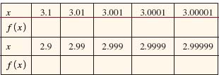
2. y = 2 is a horizontal asymptote for the graph of f
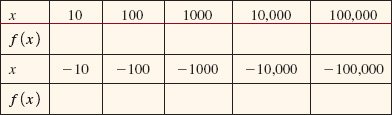
In Problems 3–22, find the vertical and horizontal asymptotes for the graph of the given rational function. Find the x- and y-intercepts of the graph. Sketch the graph of f.
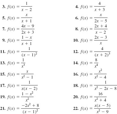
In Problems 23–30, find the vertical and slant asymptotes for the graph of the given rational function. Find the x- and y-intercepts of the graph. Sketch the graph of f.
![]()
![]()
![]()
![]()
![]()
![]()
![]()
![]()
In Problems 31–34, find the point where the graph of f crosses its horizontal asymptote. Sketch the graph of f.
![]()
![]()
![]()
![]()
In Problems 35 and 36, find the point where the graph of f crosses its slant asymptote. Use a graphing utility to obtain the graph of f and the slant asymptote in the same coordinate plane.
![]()
![]()
In Problems 37–40, find a rational function that satisfies the given conditions. There is no unique answer.
vertical asymptote: x = 2
horizontal asymptote: y = 1
x-intercept: (5, 0)
vertical asymptote: x = 1
horizontal asymptote: y = –2
x-intercept: (0, –1)
vertical asymptote: x = –1, x = 2
horizontal asymptote: y = 3
x-intercept: (3, 0)
vertical asymptote: x = 4
horizontal asymptote: y = x + 2
In Problems 41–44, find the asymptotes and any holes in the graph of the given rational function. Find the x- and y-intercepts of the graph. Sketch the graph of f.
![]()
![]()
![]()
![]()
Miscellaneous Applications
Parallel Resistors A 5-ohm resistor and a variable resistor are placed in parallel as shown in FIGURE 5.6.11. The resulting resistance R (in ohms) is related to the resistance r (in ohms) of the variable resistor by the equation
![]()
Sketch the graph of R as a function of r for r > 0. What is the resulting resistance R as r becomes very large?
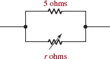
FIGURE5.6.11 Parallel resistors in Problem 45
Power The electrical power P produced by a certain source is given by
![]()
where E is the voltage of the source, R is the resistance of the source, and r is the resistance in the circuit. Sketch the graph of P as a function of r using the values E = 5 volts and R = 1 ohm.
Illumination Intensity The intensity of illumination from a light source at any point is directly proportional to the strength of the source and inversely proportional to the square of the distance from the source. Given two sources of strengths 16 units and 2 units that are 100 cm apart, as shown in FIGURE 5.6.12, the intensity I at any point P between them is given by
![]()
where x is the distance from the 16-unit source. Sketch the graph of I(x) for 0 < x < 100. Describe the behavior of I(x) as x → 0+. As x → 100–.

FIGURE 5.6.12 Two light sources in Problem 47
For Discussion
Suppose f(x) = P(x)/Q(x). Prove the symmetry rules (2), (3), and (4), for rational functions.
Construct a rational function f(x) = P(x)/Q(x) whose graph crosses its slant asymptote twice. Assume P(x) and Q(x) have no common factors.
Construct a rational function f(x) = P(x)/Q(x) whose graph has two holes in it.


A. True/False_______________________________________________
In Problems 1–18, answer true or false.
1. f(x) = 2x3 – 8x–2 is not a ploynomial.___
![]() is a rational function.___
is a rational function.___
The graph of a polynomial function can have no holes in it.___
A polynomial function of degree 4 has exactly four real zeros.___
When a polynomial of degree greater than 1 is divided by x + 2, the remainder is always a constant.___
If the coefficients a, b, c, and d of the polynomial function f(x) = ax3 + bx + cx + d are positive integers, then f has no positive real zeros.___
The polynomial equation 2x7 = 1 – x has a solution in the interval [0, 1].___
The graph of the rational function f(x) = (x2 + 1)/x has a slant asymptote.___
The graph of the polynomial function f(x) = 4x6 + 3x2 is symmetric with respect to the y-axis.___
The graph of a polynomial function that is an odd function must pass through the origin.___
An asymptote is a line that the graph of a function approaches but never crosses.___
The point ![]() is on the graph of
is on the graph of ![]() .___
.___
The graph of a rational function f(x) = P(x)/Q(x) has a slant asymptote when the degree of P is greater than the degree of Q. ___
If 3 – 4i is a zero of a polynomial function f(x) with real coefficients, then 3 + 4i is also a zero of f(x).___
A polynomial function must have at least one rational zero. ___
If 1+ i is a zero of f(x) = x3 – 6x2 + 10x – 8, then 4 is also a zero of f. ___
The continuous function f(x) = x6+ 2x5 – x2 + 1 has a real zero within the interval[–1, 1]. ___
When f(x) = x50 + 1 is divided g(x) = x – 1, the remainder is f(1) = 2. ___
B. Fill in the Blanks____________
In Problems 1–12, fill in the blanks.
The graph of the polynomial function f(x) = x3(x – 1)2(x – 5) is tangent to the x-axis at ___________ and passes through the x-axis at___________.
A third-degree polynomial function with zeros 1 and 3i is ___________.
The end behavior of the graph of f(x) = x2(x + 3)(x - 5) resembles the graph of the power function f(x) = ___________.
The polynomial function f(x) = x4 – 3x3 + 17x2 – 2x + 2 has ___________ (how many) possible rational zeros.
For f(x) = kx2(x – 2)(x – 3), f(–1) = 8 if k =___________.
The y-intercept of the graph of the rational function ![]() is ___________.
is ___________.
The vertical asymptotes for the graph of the rational function ![]() are___________.
are___________.
The x-intercepts of the graph of the rational function ![]() are___________.
are___________.
The horizontal asymptote for the graph of the rational function ![]() is___________.
is___________.
A rational function whose graph has the horizontal asymptote y = 1 and an x-intercept (3, 0) is___________.
The graph of the rational function ![]() , where n is a nonnegative integer, has the horizontal asymptote y = 0 when n = ___________.
, where n is a nonnegative integer, has the horizontal asymptote y = 0 when n = ___________.
The graph of the polynomial function f(x) = 3x5 – 4x2 + 5x – 2 has at most ___________ turning points.
C. Review Exercises________
In Problems 1 and 2, use long division to divide f(x) by g(x).
f(x) = 6x5 – 4x3 + 2x2 + 4, g(x) = 2x2 – 1
f(x) = 15x4 – 2x3 + 8x + 6, g(x) = 5x3 + x + 2
In Problems 3 and 4, use synthetic division to divide f(x) by g(x).
f(x) = 7x4 – 6x2 + 9x + 3, g(x) = x – 2
f(x) = 4x3 + 7x2 – 8x, g(x) = x + 1
Without actually performing the division, determine the remainder when f(x) = 5x3 – 4x2 + 6x – 9 is divided by g(x) = x + 3.
Use synthetic division and the Remainder Theorem to find f(c) for f(x) = x6 – 3x5 + 2x4 + 3x3 – x2 + 5x – 1 when c = 2.
Determine the values of the positive integer n such that f(x) = xn + cn is divisible by g(x) = x + c.
Suppose that
f(x) = 36x98 – 40x25 + 18x14 – 3x7 + 40x4 + 5x2 – x + 2
is divided by g(x) = x – 1. What is the remainder?
List, but do not test, all possible rational zeros of
f(x) = 8x4 + 19x3 + 31x2 + 38x – 15.
Find the complete factorization of f(x) = 12x3 + 16x2 + 7x + 1.
In Problems 11 and 12, verify that each of the indicated numbers is a zero of the given polynomial function f(x). Find all other zeros and then give the complete factorization of f(x).
2; f(x) = (x – 3)3 + 1
–1; f(x) = (x + 2)4 – 1
In Problems 13–16, find the real value of k so that the given condition is satisfied.
The remainder in the division of f(x) = x4 – 3x3 – x2 + kx – 1 by g(x) = x – 4 is r = 5.
x + ![]() is a factor of f(x) = 8x2 – 4kx + 9.
is a factor of f(x) = 8x2 – 4kx + 9.
x – k is a factor of f(x) = 2x3 + x2 + 2x – 12.
The graph of ![]() has a hole at x = k.
has a hole at x = k.
In Problems 17 and 18, find a polynomial function f of indicated degree whose graph is given in the figure.
fifth degree
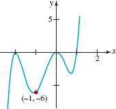
FIGURE 5.8.1Graph for Problem 17
sixth degree
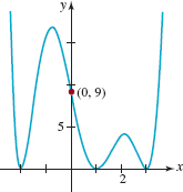
FIGURE 5.8.2 Graph for Problem 18
In Problems 19–28, match the given rational function with one of the graphs (a)–(j).
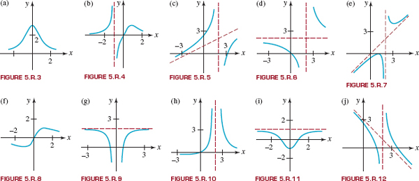
![]()
![]()
![]()
![]()
![]()
![]()
![]()
![]()
![]()
![]()
In Problems 29 and 30, find the asymptotes for the graph of the given rational function. Find the x- and y-intercepts of the graph. Sketch the graph of f.
![]()
![]()
Discuss: Without graphing or attempting to find them, why does the polynomial function
![]()
have no real zeros?
Sketch the graph of ![]() From the graph of f, find the solution of the inequality
From the graph of f, find the solution of the inequality
![]()
(a) Show that the number ![]() is a zero of the polynomial function f(x) = x4 – 10x2 + 1.
is a zero of the polynomial function f(x) = x4 – 10x2 + 1.
(b) Discuss: How does part (a) prove that ![]() is an irrational number?
is an irrational number?
Consider the polynomial function f(x) = x3 – i, where ![]() .
.
(a) Verify that each of the three numbers ![]() is zero of the function f.
is zero of the function f.
(b) Note in part (b) that each zero is not the conjugate of either of the two remaining zeros. Explain why this does not violate the Conjugate Zero Theorem in Section 5.3.
** A prime number is a positive integer greater than 1 whose only positive integer factors are itself and the number 1. The first five prime numbers are 2, 3, 5, 7, and 11.
*** If we want an approximation that is accurate to two decimal places, we calculate the midpoints mi, i = 1, 2,…, n until the error becomes less than 0.005.