
9 Matrices and Determinants
In This Chapter
5.9 Linear Systems: Augmented Matrices
6.9 Linear Systems: Matrix Inverses
7.9 Linear Systems: Determinants

A rectangular array of numbers or symbols is called a matrix.
A Bit of History The focus of this chapter will be on three topics: matrices, determinants, and systems of equations. We will see how the first two concepts can be used to solve systems of n linear equations in n unknowns.
Matrices were the invention of the eminent English mathematicians Arthur Cayley (1821-1895) and James Joseph Sylvester (1814-1897). As with many mathematical inventions, the theory and algebra of matrices grew as an offshoot of Cayley's primary mathematical interest and investigations. Cayley was a child prodigy in mathematics and excelled in that subject as a student at Trinity College at Cambridge. However, for want of a job in mathematics, he became a lawyer at the age of 28. After enduring 14 years in this profession, he was offered a professorship of mathematics at Cambridge in 1863, where he was influential in getting the first women admitted to Cambridge. Arthur Cayley also invented the concept of n-dimensional geometry and made many significant contributions to the theory of determinants. During 1881-1882, Cayley taught in the United States at Johns Hopkins University. Sylvester also taught at Johns Hopkins University from 1877 to 1883.
9.1 Introduction to Matrices
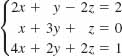
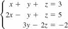
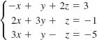
![]() Introduction The method of solution, and the solution itself, of a system of linear equations does not depend in any way on what symbols are used as variables. In Example 2 of Section 8.1, we saw that the solution of the system
Introduction The method of solution, and the solution itself, of a system of linear equations does not depend in any way on what symbols are used as variables. In Example 2 of Section 8.1, we saw that the solution of the system
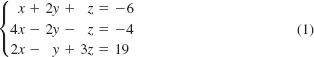
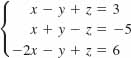
is x = –2, y = –5, z = 6 or as an ordered triple (–2, –5, 6).This same ordered triple is also a solution of
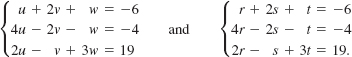
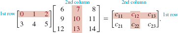
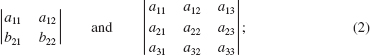
The point is this: The solution of a system of linear equations depends only on the coefficients and constants that appear in the system and not on what symbols are used to represent the variables. We will see that we could solve (1) by suitable manipulations on the array of numbers
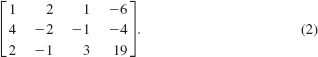
In (2) the first, second, and third columns represent the coefficients of x, y and z, respectively in (1), and the last column consists of the constants to the right of the equality sign in (1).
Before examining this idea we need to develop a mathematical system whose elements are arrays of numbers. A rectangular array such as (2) is called a matrix.
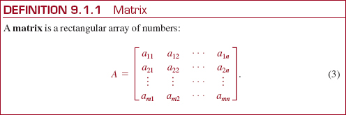
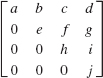
![]() Terminology If there are m rows and n columns, we say that the dimension, or size, of the matrix is m × n, and we refer to it as an “m by n matrix,” or simply, as a rectangular matrix. The matrix in (3) is an m × n matrix. An n × n matrix is called a square matrix and is said to be of order n. The entry, or element, in the i th row and j th column of an m × n matrix A is denoted by the symbol aij. Thus the entry in, say, the third row and fourth column of a matrix A is a34.
Terminology If there are m rows and n columns, we say that the dimension, or size, of the matrix is m × n, and we refer to it as an “m by n matrix,” or simply, as a rectangular matrix. The matrix in (3) is an m × n matrix. An n × n matrix is called a square matrix and is said to be of order n. The entry, or element, in the i th row and j th column of an m × n matrix A is denoted by the symbol aij. Thus the entry in, say, the third row and fourth column of a matrix A is a34.
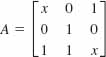
EXAMPLE 1 Dimensions
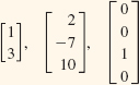
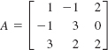
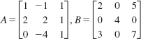
(a) The dimensions of the matrices
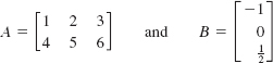
are, respectively, 2 × 3 and 3 × 1.
(b) The 2 × 2 matrix
![]()
is also referred to as a square matrix of order 2.
A 1 × n matrix consists of one row and n columns and is called a row matrix or row vector. On the other hand, an m × 1 matrix has m rows and one column and is naturally called a column matrix or column vector. The 3 × 1 matrix B in part (a) of Example 1 is a column matrix.
![]() Matrix Notation To save time and space in writing, it is convenient to use a special notation for a general matrix. An m × n matrix A is often abbreviated as A = (aij) m × n.
Matrix Notation To save time and space in writing, it is convenient to use a special notation for a general matrix. An m × n matrix A is often abbreviated as A = (aij) m × n.
EXAMPLE 2 Find the Matrix
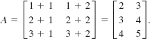
Determine the matrix A = (aij)3 × 2 if aij = i + j for each i and j.
Solution To obtain the entry in the first row and first column, we let i = 1 and j = 1; that is, a11 = 1 + 1 = 2. The remaining entries are obtained in a similar fashion:
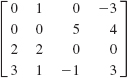
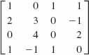
The entries a11, a22, a33,…, ann in a square matrix are said to be on the main diagonal of the matrix. For example, the main diagonal entries of the square matrices.
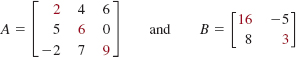
are highlighted in red.
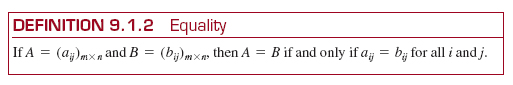
![]() Equality Two matrices are equal if they have the same dimension and if their corresponding entries are equal.
Equality Two matrices are equal if they have the same dimension and if their corresponding entries are equal.
EXAMPLE 3 Equality of Two Matrices
From Definition 9.1.2, we have the equality
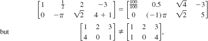
since the corresponding entries in the second row are not all equal. Also,
![]()
since the matrices do not have the same dimension.
EXAMPLE 4 Matrix Equation
Solve for x and y if
![]()
Solution From Definition 9.1.2, we equate corresponding entries. It follows that
![]()
Solving these equations gives y = –1 and x = 2
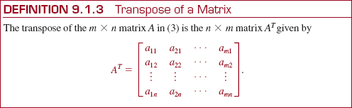
In other words, the rows of a matrix A become the columns of its transpose AT.
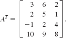
EXAMPLE 5 Transpose
Find the transpose of (a) 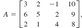 and (b) B = [5 3].
Solution (a) Since A is a 3 × 4 matrix its transpose AT will be a 4 × 3 matrix. In forming the transpose, we write the first row as the first column, the second row as the second column, and so on. Hence,
(b) The transpose of a row matrix becomes a column matrix:
![]()
As we will see in Section 9.4, the transpose of a square matrix is particularly useful.
9.1 Exercises Answers to selected odd-numbered problems begin on page ANS-22.
In Problems 1–10, state the dimension of the given matrix.
1. 
2. ![]()
3. 
4. 
5. [8]
6. [0 5 –7]
7. ![]()
8. ![]()
9. (aij)5 × 7
10. (aij)6 × 6
In Problems 11–16, suppose that a matrix A = (aij)3 × 4 is defined by
Find the indicated number.
11. a13
12. a32
13. a24
14. a33
15. 2a11 + 5a31
16. a23 – 4a33
In Problems 17–22, determine the matrix (aij)2 × 3 satisfying the given condition.
17. aij = i – j
18. aij = ij
19. aij2
20. aij = 2i + 3j
21. ![]()
22. aij = ij
In Problems 23–26, determine whether the given matrices are equal.
23. ![]()
24. [0 0], [0 0 0]
25. ![]()
26. ![]()
In Problems 27–32, solve for the variables.
27. ![]()
28. ![]()
29. ![]()
30. ![]()
31. ![]()
32. ![]()
In Problems 33–38, find the transpose of the given matrix.
33. ![]()
34. [– 1 6 7]
35. ![]()
36. 
37. 
38. 
In Problems 39 and 40, verify that the given matrix is symmetric. An n ×n matrix A is said to be symmetric if AT = A.
39. ![]()
40. 
For Discussion
41. Give an example of a 4 × 4 matrix that is symmetric. See Problem 39.
42. Suppose AT is the transpose of the matrix A. Discuss: What is (AT)T?
9.2 Algebra of Matrices
![]() Introduction In ordinary algebra, we take for granted the fact that two real numbers can be added, subtracted, and multiplied. In matrix algebra, however, two matrices can be added, subtracted, and multiplied only under certain conditions.
Introduction In ordinary algebra, we take for granted the fact that two real numbers can be added, subtracted, and multiplied. In matrix algebra, however, two matrices can be added, subtracted, and multiplied only under certain conditions.
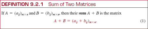
![]() Addition of Matrices Only matrices that have the same dimensions can be added. If A and B are both m × n matrices, then their sum A + B is the m × n matrix formed by adding the corresponding entries in each matrix. In other words, the entry in the first row and first column of A is added to the entry in the first row and first column of B, and so on. Using symbols we have the following definition.
Addition of Matrices Only matrices that have the same dimensions can be added. If A and B are both m × n matrices, then their sum A + B is the m × n matrix formed by adding the corresponding entries in each matrix. In other words, the entry in the first row and first column of A is added to the entry in the first row and first column of B, and so on. Using symbols we have the following definition.
If matrices A and B have different dimensions, then they cannot be added.
EXAMPLE 1 Sum of Two Matrices
(a) Because the two matrices
![]()
have the same dimension (namely, 2 × 3) we can add them to obtain a third matrix with the same dimension:
![]()
(b) Because the two matrices
![]()
have different dimensions (respectively, 2 × 3 and 2 × 2) we cannot add them.
It follows directly from the properties of real numbers and Definition 9.2.1 that the operation of addition on the set of m × n matrices possesses the following two familiar properties:
![]()
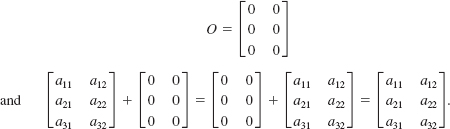
![]() Additive Identity A matrix whose entries are all zeros is said to be a zero matrix and is denoted by O. If A and O are m × n matrices, then we have A + O = O + A = A for every m × n matrix A. We say that the m × n zero matrix O is the additive identity for the set of m × n matrices. For example, for the set of 3 × 2 matrices the zero matrix is
Additive Identity A matrix whose entries are all zeros is said to be a zero matrix and is denoted by O. If A and O are m × n matrices, then we have A + O = O + A = A for every m × n matrix A. We say that the m × n zero matrix O is the additive identity for the set of m × n matrices. For example, for the set of 3 × 2 matrices the zero matrix is
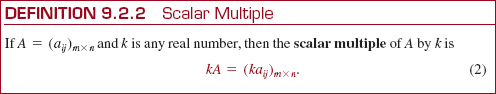
![]() Scalar Multiple In the discussion of matrices, real numbers are referred to as scalars. If k is a real number, then the scalar multiple of a matrix A and a real number k is the matrix kA with each entry equal to the product of the real number k and the corresponding entry in the given matrix.
Scalar Multiple In the discussion of matrices, real numbers are referred to as scalars. If k is a real number, then the scalar multiple of a matrix A and a real number k is the matrix kA with each entry equal to the product of the real number k and the corresponding entry in the given matrix.
EXAMPLE 2 Scalar Multiple
For k = 3 and ![]() it follows from Definition 9.2.2 that
it follows from Definition 9.2.2 that
![]()
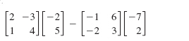
EXAMPLE 3 Sum of Two Scalar Multiples
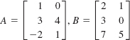
Consider 2 × 3 the matrices ![]() Find
Find
(a) (–1)A + 2B, and (b) (–1)A + A
Solution (a) Applying Definition 9.2.2, we have the scalar multiples
![]()
Using the foregoing results, we have from Definition 9.2.1,
![]()
(b) 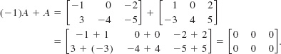
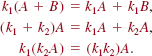
The following properties of the scalar product are readily established using Definitions 9.2.1 and 9.2.2. If k1 and k2 are scalars, then
![]() Additive Inverse As Example 3 shows, the additive inverse –A of the matrix A is defined to be the scalar multiple (– 1)A. Thus, if O is the m × n zero matrix,
Additive Inverse As Example 3 shows, the additive inverse –A of the matrix A is defined to be the scalar multiple (– 1)A. Thus, if O is the m × n zero matrix,
![]()
for any m × n matrix A. We use the additive inverse to define subtraction, or the difference A – B, of two m × n matrices A and B as follows:
![]()
we see that the difference is obtained by subtracting the entries in B from the corresponding entries in A.
EXAMPLE 4 Difference
The two row matrices
![]()
have the same dimension (namely, 1 × 3) and so their difference is
![]()
EXAMPLE 5 Difference
If 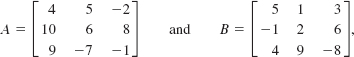
find A – B and B – A
Solution
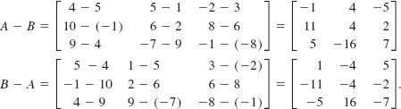
Example 5 illustrates that B – A = –(A – B).
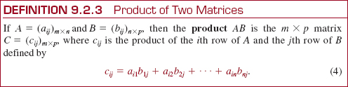
![]() Multiplication of Two Matrices In order to find the product AB of two matrices A and B, we require that the number of columns in A be equal to the number of rows in B. Suppose A = (aij)m × n is an m × n matrix and B = (bij)n × p is an n × p matrix. As illustrated below, to find the entry cij in the product C = AB, we pair the numbers in the i th row of A with those in the j th column of B. We then multiply the pairs and add the products, as follows:
Multiplication of Two Matrices In order to find the product AB of two matrices A and B, we require that the number of columns in A be equal to the number of rows in B. Suppose A = (aij)m × n is an m × n matrix and B = (bij)n × p is an n × p matrix. As illustrated below, to find the entry cij in the product C = AB, we pair the numbers in the i th row of A with those in the j th column of B. We then multiply the pairs and add the products, as follows:
![]()
that is,
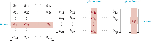
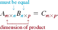
We say that (3) is the product of the ith row of A and the j th row of B. It follows from (3) that the product AB has m rows and p columns. In other words, the dimension of the product C = AB is determined from the number of rows in A and the number of columns in B:
For example, the product of a 2 × 3 matrix and a 3 × 3 matrix is a 2 × 3 matrix:
The entry, say, c12 is the product of the first row in A and second column of B:
![]()
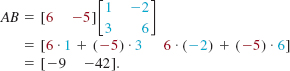
We summarize the foregoing discussion with a formal definition.
Although at first inspection the definition of the product of two matrices may seem unnatural, it does have many applications. For example, in Section 9.6, it will provide us with a new technique for solving some system of equations.
EXAMPLE 6 Product
In other words, the number of columns in A equals the number of rows in B![]() .
.
If ![]() then by inspection we see that A and B are conformable to multiplication in the order AB because the dimension of A is 1 × 2 and the dimension of B is 2 × 2. It follows from Definition 9.2.3 that
then by inspection we see that A and B are conformable to multiplication in the order AB because the dimension of A is 1 × 2 and the dimension of B is 2 × 2. It follows from Definition 9.2.3 that
It is possible for the product AB to exist even though the product BA may not be defined. In Example 6, because the number of columns in B (that is, 2) does not equal the number of rows in A (that is, 1), the product BA is not defined.
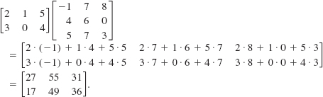
EXAMPLE 7 Product
If 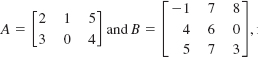 and find the product AB.
Solution Using Definition 9.2.3, we have
EXAMPLE 8 Comparing AB and BA
If ![]() find the products AB and BA.
find the products AB and BA.
Solution Because A and B are both of dimension 2 × 2 we can form the products AB and BA:

Note in Example 8 that even though both products AB and BA are defined, we have ![]() . In other words, matrix multiplication is not, in general, commutative. However, it can be demonstrated that matrix multiplication does possess the following properties:
. In other words, matrix multiplication is not, in general, commutative. However, it can be demonstrated that matrix multiplication does possess the following properties:
provided these sums and products are defined. See Problems 23–26 in Exercises 9.2.
![]() Identity Matrix The set of all square matrices of a given order n has a multiplicative identity, that is, there is a unique n × n matrix In such that
Identity Matrix The set of all square matrices of a given order n has a multiplicative identity, that is, there is a unique n × n matrix In such that
![]()
for any n × n matrix A. We say that In is the identity matrix of order n, or simply, the identity matrix. It can be shown that each entry on the main diagonal of In is 1 and all other entries are 0:
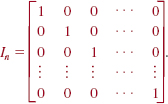
For example,
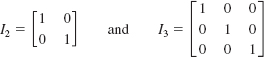
are identity matrices of orders 2 and 3, respectively.
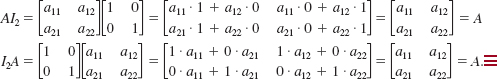
EXAMPLE 9 Identity for the Set of 2 × 2 Matrices
Verify that ![]() is the multiplicative identity for the set of 2 × 2 matrices.
is the multiplicative identity for the set of 2 × 2 matrices.
Solution Let ![]() be a 2 × 2 matrix. Then
be a 2 × 2 matrix. Then
NOTES FROM THE CLASSROOM

A 1 × n matrix, or row matrix, and an m × 1 matrix, or column matrix,
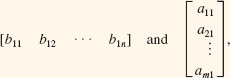
are also called a row vector and a column vector, respectively. For example,
![]()
are row vectors, and
are column vectors.
Suppose A is a 1 × n row vector and B is an n × 1 column vector, that is, A has the same number of columns as the row matrix B has rows, then the product AB is a 1 × 1 matrix or a scalar. We also say that AB is the inner product of the two matrices. For example, if ![]() then their inner product is
then their inner product is
![]()
That is what is going on in (4): If A is an m × n matrix and B is an n × p matrix, then the m × p matrix AB is formed by taking the inner product of each row vector in A with all the column vectors in B.
9.2 Exercises Answers to selected odd-numbered problems begin on page ANS-22.
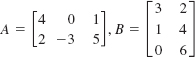
In Problems 1–10, find A + B, A – B, 4A, and 3A – 2B.
1. ![]()
2. ![]()
3. ![]()
4. 
5. ![]()
6. ![]()
7. A = [10 3],B = [4 –5]
8. A = [5],B = [2]
9. ![]()
10. ![]()
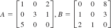
In Problems 11–20, find AB and BA, if possible.
11. ![]()
12. ![]()
13. 
14. 
15. 
16. 
17. ![]()
18. ![]()
19. ![]()
20. 
In Problems 21 and 22, find A2 = AA for the given matrix A.
21. ![]()
22. 
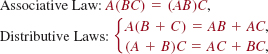
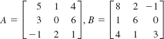
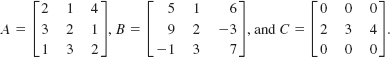
In Problems 23–26, find the given matrix if
![]()
23. A(BC)
24. C(BA)
25. A(B + C)
26. B(C – A)
In Problems 27 and 28, write the given sum as a single column matrix.
27. 
28. 
In Problems 29–32, give the dimension of the matrix A so that the following products are defined.
29. 
30. 
31. 
32. 
In Problems 33 and 34, find c23 and c12 for the matrix C = 2A – 3B.
33. ![]()
34. 
35. Verify that the polynomial in two variables ax2 + bxy + cy2 is the same as the matrix product
![]()
36. Write ![]() without matrices.
without matrices.
In Problems 37 and 38, find a 2 × 2 matrix X that satisfies the given equation.
37. ![]()
38. ![]()
In Problems 39–42, suppose ![]() Verify the given property of the transpose by computing the left and right members of the given equality.
Verify the given property of the transpose by computing the left and right members of the given equality.
39. (A + B)T = AT + BT
40. (A – B)T = AT – BT
41. (AB)T = BTAT
42. (6A)T = 6AT
Miscellaneous Applications
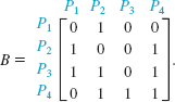
43. Spread of a Disease Two persons X and Y have infectious hepatitis. They have the possibility of contact, and thus of passing on the disease, with four persons P1, P2, P3, and P4. Let a 2 × 4 matrix be given as follows:
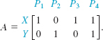
If person X (or Y) has contact with any of the four persons, a 1 is entered in the row labeled X (or Y) in the appropriate column. If X (or Y) has no contact with a particular person, a 0 is entered. Define the contacts between P1, P2, P3, and P4 with four additional persons P5, P6, P7, and P8 by
Compute the product AB and interpret the entries.
44. Revenue The revenue, in thousands of dollars, for three successive weeks for five stores in a grocery chain are represented by the entries in the following matrices R1, R2, and R3:
![]()
Over the same period the costs can be represented by
![]()
Compute the matrix 4R1 – 3.5C1 and interpret the entries.
45. Retailing A retail store purchased two brands of stereophonic equipment consisting of amplifiers, tuners, and speakers from wholesale outlets. Because of limited quantities, the store must purchase these supplies from three wholesale dealers. Matrix A gives the wholesale price of each piece of equipment in dollars. Matrix B represents the number of units of each piece of equipment purchased. (For example, b11 = 1 means that one amplifier, one tuner, and one set of speakers of brand 1 is purchased from wholesale dealer 1.)
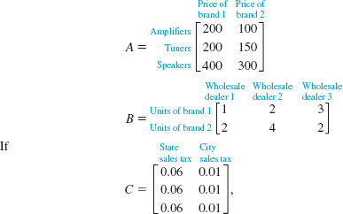
find the matrix P = (AB)C, and interpret the significance of its entries.
46. Investigative Reporting A television station does a weekly comparison of three supermarkets for the costs of five basic food items. In a particular week, the following matrix gives the per-pound price for each item:
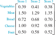
The number of pounds purchased of each items is given by the matrix
![]()
By an appropriate matrix multiplication, compare the total costs at the three stores.
47. Inventory A company owns five tire stores. The inventory of tires in store S1 is given by
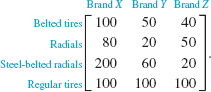
Stores S2 and S3 each have 3 times as many tires as S1; store S4 has ½ as many tires as stores S1; and store S5 has 2 times as many tires as S1. Find the matrix that gives the total inventory of tires that the company owns.
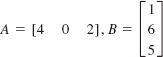
48. Distance Traveled The velocities of cars X, Y, and Z in kilometers per hour are given in the 3 × 1 matrix

The number of hours each car travels is given in the 1 × 3 matrix B = [3 4 6]. Compute the products AB and BA and interpret the entries in each.
49. College Dropouts A college has 3000 students enrolled at the beginning of a particular academic year. A breakdown by classes is given by the matrix
![]()
It is projected that the percentage of dropouts per class, in any given year, is given by

That is to say, 20% of the freshmen class is expected to leave school before the completion of the year, and so on. Using matrix multiplication, determine the projected total number of dropouts for that particular year.
For Discussion
50. Show by example that, in general, for n × n matrices A and B,
![]()
[Hint: Use 2 × 2 matrices and A2 = AA and B2 = BB.]
51. Let A and B be 2 × 2 matrices. Is it true, in general, that
![]()
Explain.
52. Find two different 2 × 2 matrices A, where A ≠ O, for which A2 = O.
53. Suppose A = ![]() . Find a 2 × 2 matrix B, such that AB = BA = I2.
. Find a 2 × 2 matrix B, such that AB = BA = I2.
54. If a, b, and c are real numbers and c ≠ 0, then ac = bc implies a = b. For matrices, AC = BC does not imply A = B. Verify this for the matrices
9.3 Determinants
![]() Introduction To each square matrix A, we can associate a number called the determinant of A. For example, the determinants of 2 × 2 and 3 × 3 matrices
Introduction To each square matrix A, we can associate a number called the determinant of A. For example, the determinants of 2 × 2 and 3 × 3 matrices
are written
![]() Even though a determinant is a number it is often convenient to think of it as a square array. Thus, for example, second-order and third-order determinants are, in turn, referred to as 2 × 2 and 3 × 3 determinants.
Even though a determinant is a number it is often convenient to think of it as a square array. Thus, for example, second-order and third-order determinants are, in turn, referred to as 2 × 2 and 3 × 3 determinants.
in other words, the brackets are replaced by vertical bars. A determinant of an n × n matrix is said to be a determinant of order n or an nth-order determinant. The determinants in (2) are, in turn, determinants of orders 2 and 3. In a discussion, the determinant of a square matrix A is denoted by symbols such as det A or | A |. We will use the former symbol exclusively. Thus, if
![]()
We will examine two applications of determinants in Sections 9.4 and 9.7.
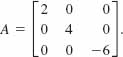
![]() Determinant of a 2 × 2 Matrix As we just indicated, a determinant is a number. We begin with the definition of the determinant of order 2, that is, the determinant of a 2 × 2 matrix.
Determinant of a 2 × 2 Matrix As we just indicated, a determinant is a number. We begin with the definition of the determinant of order 2, that is, the determinant of a 2 × 2 matrix.
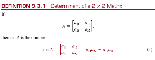
EXAMPLE 1 Determinant of Order 2
Evaluate the determinant of the matrix
![]()
Solution From (3),
![]()
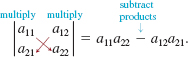
As a mnemonic for the formula in (3), remember that the determinant is the difference of the products of the diagonal elements:
Determinants of 2 × 2 matrices play a fundamental role in the evaluating of determinants of n × n matrices for n > 2. In general, a determinant of an n × n matrix can be expressed in terms of determinants of (n - 1) × (n -1) matrices, that is, determinants of order n -1. Thus, for example, the determinant of a 3 × 3 matrix can be expressed in terms of determinants of order 2. In preparation for a method of evaluating a determinant of an n × n matrix, n 2, we need to introduce the notion of a cofactor determinant.
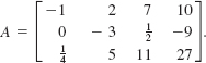
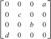
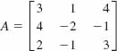
![]() Minor and Cofactor If aij denotes the entry in the ith row and jth column of a square matrix A, then the minor Mij of aij is defined to be the determinant of the matrix obtained by deleting the i th row and the j th column of A. Thus for the matrix
Minor and Cofactor If aij denotes the entry in the ith row and jth column of a square matrix A, then the minor Mij of aij is defined to be the determinant of the matrix obtained by deleting the i th row and the j th column of A. Thus for the matrix
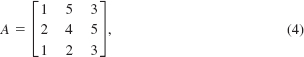
the minors of a11 = 1, a12 = 5, a22 = 4, and a32 = 2 are, in turn, the determinants
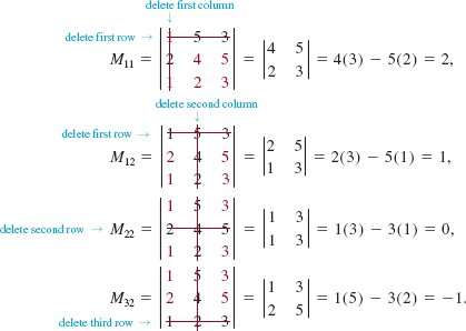
The cofactor Aij of the entry aij is defined to be the minor Mij multiplied by (-1)i+j, that is,
![]() (-1)i+j is 1 if i + j is even, (-1)i+j is -1 if i + j is odd.
(-1)i+j is 1 if i + j is even, (-1)i+j is -1 if i + j is odd.
![]()
Thus for the matrix A in (4) the cofactors associated with the foregoing minor determinants are
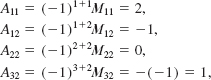
and so on. For a 3 × 3 matrix, the coefficient (-1)i+j of the minor Mij follows the pattern
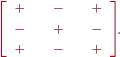
This “checkerboard” pattern of signs extends to matrices of larger size as well.
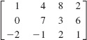
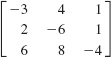
EXAMPLE 2 Cofactors
For the matrix
find the cofactor of the given entry: (a) 0 (b) 7 (c) -1.
Solution (a) The number 0 is the entry ofthe first row (i = 1) and third column (j = 3). From (5) the cofactor of 0 is the determinant
![]()
(b) The number 7 is the entry in the second row (i = 2) and third column (j = 3). Thus the cofactor is
![]()
(c) Finally, because -1 is the entry in the third row (i = 3) and first column (j = 1), its cofactor is
![]()
We are now in a position to evaluate the determinant of any square matrix.
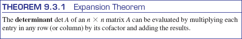
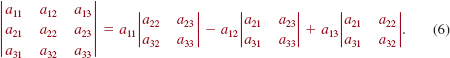
When we use Theorem 9.3.1 to find the value of the determinant of a square matrix A, we say that we have expanded the determinant of A by a given row or by a given column. For example, the expansion of the determinant of the 3 × 3 matrix in (1) by the first row is
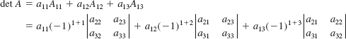
or
EXAMPLE 3 Expansion by the First Row
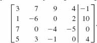
Evaluate the determinant of the 3 × 3 matrix
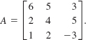
Solution Using the expansion by the first row given in (6) we have
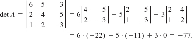
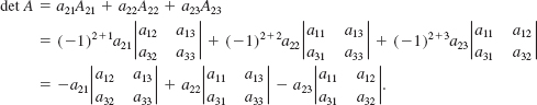
Theorem 9.3.1 states that the determinant of a square matrix A can be expanded by any row or any column. For example, the expansion of the determinant of the 3 × 3 matrix in (1) by, say, the second row gives
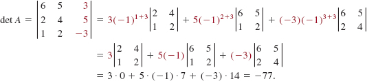
EXAMPLE 4 Example 3 Revisited
The expansion of the determinant in Example 3 by the third column is
In the expansion of a determinant, since the entries in a row (or column) multiply the cofactors of that row (or column), it makes sense that if a determinant has a row (or column) with several zero entries that we expand the determinant by that row (or column).
EXAMPLE 5 Determinant of Order 4
Evaluate the determinant of the 4 × 4 matrix
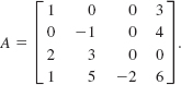
Solution Since the third column has only one nonzero entry, we expand the det A by the third column:
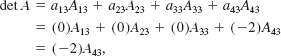
where the cofactor A43 is
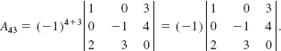
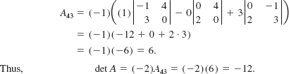
Using (6), we expand the last determinant by the first row:
![]() Properties Determinants have many special properties, some of which are given in the following theorem.
Properties Determinants have many special properties, some of which are given in the following theorem.
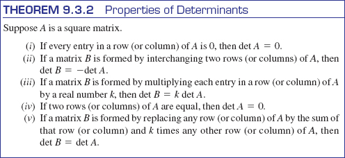
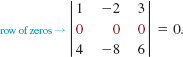
It is easy to prove part (i) of Theorem 9.3.2 from Theorem 9.3.1: We expand det A by the row (or column) that contains all zero entries. As exercises, you will be asked to verify parts (ii)-(v) of Theorem 9.3.2 for matrices of order 2. See Problems 31-34 in Exercises 9.3.
EXAMPLE 6 Using Theorem 9.3.2
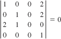
Without expanding, it follows immediately from (i) of Theorem 9.3.2 that
EXAMPLE 7 Using Theorem 9.3.2
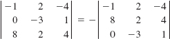
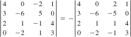
It follows from (ii) of Theorem 9.3.2 that
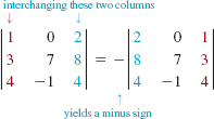
by interchanging the first column and the third column.
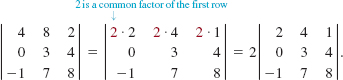
EXAMPLE 8 Using Theorem 9.3.2
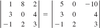
By factoring 2 from each entry in the first row, it follows from (iii) of Theorem 9.3.2 that
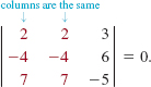
EXAMPLE 9 Using Theorem 9.3.2
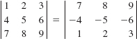
Because the first and second columns are the same, it follows from (iv) of Theorem 9.3.2 that
As the next example shows, using (v) of Theorem 9.3.2 can simplify the evaluation of a determinant.
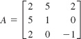
EXAMPLE 10 Using Theorem 9.3.2
Evaluate the determinant of the 3 × 3 matrix
Solution We use (v) of Theorem 9.3.2 to obtain a matrix, with the same determinant, that has a row (or column) with only one nonzero entry. To avoid fractions, it is best to use a row (or column) containing the element 1 or -1, if possible. Thus we will use the first row to introduce zeros into the first column as follows. We multiply the first row by 2 and add the result to the second and obtain

Now multiplying the first row by -3 and adding the result to the third row gives
Expanding (8) by the first column, we find that

From (v) of Theorem 9.3.2, it follows that the determinant of the matrix given in (7) has the same value; that is, det A = 19.
9.3 Exercises Answers to selected odd-numbered problems begin on page ANS-22.
In Problems 1-4, find the minor and the cofactor of each element in the given matrix.
1. ![]()
2. ![]()
3. 
4. 
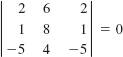
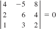
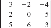
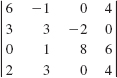
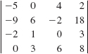
In Problems 5-18, evaluate the determinant of the given matrix. In Problem 10, assume that the numbers a and b are nonzero.
5. ![]()
6. ![]()
7. ![]()
8. ![]()
9. ![]()
10. 
11. 
12. 
13. 
14. 
15. 
16. 
17. 
18. 
In Problems 19-26, state why the equality is true without evaluating the given determinant.
19. 
20. ![]()
21. 
22. 
23. 
24. 
25. 
26. 
In Problems 27-30, use (v) of Theorem 9.3.2 to introduce zeros, as in Example 10, before evaluating the given determinant.
27. 
28. 
29. 
30. 
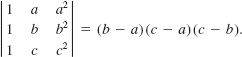
In Problems 31-34, verify the given identity by expanding each determinant.
31. ![]()
32. ![]()
33. ![]()
34. ![]()
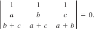
35. Prove that
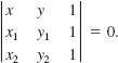
36. Verify that an equation of the line through the points (x1, y1), (x2, y2) is given by
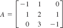
In Problems 37-40, find the values of λ for which det(A-λ/n) = 0. These numbers are called the eigenvalues of the matrix A.
37. ![]()
38. ![]()
39. 
40. 
41. Without expanding, state why
42. Verify that det (AB) = det A.det B for the 2 × 2 matrices
![]()
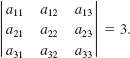
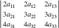
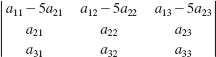
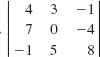
In Problems 43-48, find the value of each determinant given that
43. 
44. 
45. 
46. 
47. 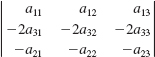
48. 
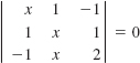
In Problems 49 and 50, solve for x.
49. 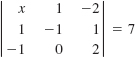
50. 
For Discussion
51. Without expanding the determinant of the matrix
where a, b, and c are nonzero constants, explain why det A = 0.
52. Let A be a square matrix and let AT be its transpose. Discuss: Are det A and det AT related in any way?
9.4 Inverse of a Matrix
![]() Introduction In ordinary algebra, every nonzero real number a has a multiplicative inverse b such that
Introduction In ordinary algebra, every nonzero real number a has a multiplicative inverse b such that
![]()
where the number 1 is the multiplicative identity. The number b is the reciprocal of the number a, that is, a-1 = 1/a. Similarly, a matrix A can have a multiplicative inverse, but as we see in the discussion that follows A has to be a certain kind of square matrix.
![]() Multiplicative Inverse IfA is an n × n matrix and ifthere exists an n × n matrix B such that
Multiplicative Inverse IfA is an n × n matrix and ifthere exists an n × n matrix B such that
![]()
we say that B is the multiplicative inverse, or simply the inverse, of A. The multiplicative inverse of A is written B = A-1. Unlike in the real number system, we note that the symbol A-1 does not denote the reciprocal of A, that is, A-1 is not 1/A. In matrix theory, 1/A is not defined. A square matrix that has a multiplicative inverse is said to be nonsingular or invertible. When a square matrix A has no inverse, it is said to be singular or noninvertible.
EXAMPLE 1 Inverse of a Matrix
if A = ![]() and B =
and B = ![]()
then
![]()
and
![]()
Because AB = BA = I2 we conclude from (1) that the matrix A is nonsingular and that the inverse A-1 of the matrix A is the given matrix B.
![]() Finding A-1: Method 1 We can find the inverse of a nonsingular matrix by two different methods. The first method considered uses determinants. We begin with the special case where A is a 2 × 2 matrix:
Finding A-1: Method 1 We can find the inverse of a nonsingular matrix by two different methods. The first method considered uses determinants. We begin with the special case where A is a 2 × 2 matrix:
![]()
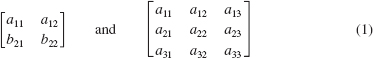
In order for a 2 × 2 matrix
![]()
to be the inverse of A, we must have
![]()
By multiplication and equality of matrices, we find that b11 and b21 must satisfy the linear system
![]()
while b12 and b22 must satisfy
![]()
Solving these two systems of equations gives
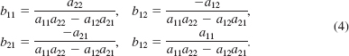
An inspection of the expressions in (4) reveals that the denominator in each fraction is the value of the determinant of the matrix A, that is
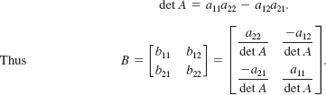
This result leads to the following theorem.
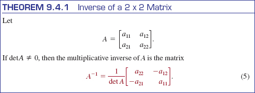
From the derivation preceding Theorem 9.4.1, we have shown that AA-1 = I2. We leave it as an exercise to verify that A-1A = I2, where A-1 is given by (5). See Problem 34 in Exercises 9.4.
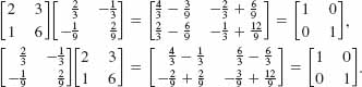
EXAMPLE 2 Using (5)
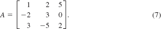
Find A-1 for
![]()
Solution First, we calculate the determinant of the matrix:
![]()
With the identifications a11 = 3, a12 = 2, a21 = -7, and a22 = -4 we see from (5) of Theorem 9.4.1 that the inverse of the matrix A is
![]()
Theorem 9.4.1 is a special case of the next theorem, which we state without proof. Before reading Theorem 9.4.2 you are encouraged to review Definition 9.1.3 on the transpose of a matrix.
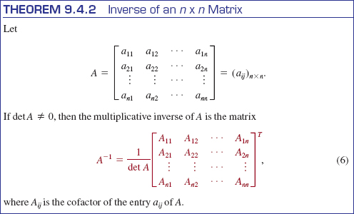
The transpose of the matrix of cofactors,
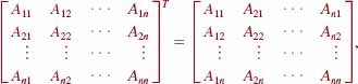
given in (6) is called the adjoint of the matrix A and is denoted by adj A. In the adjoint matrix given in (6), it is important to note that the entries a ij of the matrix A are replaced by their corresponding cofactors Aij and then we take the transpose of that matrix. The inverse in (6) can be written
![]()
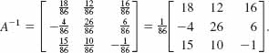
EXAMPLE 3 Using (6)
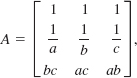
Find A -1 for
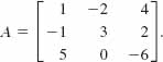
Solution The determinant of A is det A = -86. Now, for each entry in A the corresponding cofactor is
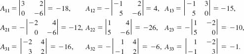
Thus by (6) of Theorem 9.4.2, the inverse of A is ![]() times the adjoint of the matrix A:
times the adjoint of the matrix A:

In Theorems 9.4.1 and 9.4.2, we saw that we could calculate A -1provided det A ≠ 0. Conversely, if A-1 exists, then it can be shown that det A ≠ 0. We conclude:
![]()
EXAMPLE 4 Using (7)
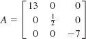
The matrix
![]()
has no inverse because det A = 8 – 8 = 0. Thus by (7), A is a singular matrix.
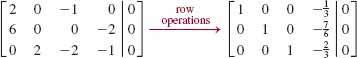
It should be apparent that the use of (6) becomes formidable for matrices of order n > 3. For example, for a 4 × 4 matrix we must first compute sixteen determinants of order 3. A more efficient method for finding the multiplicative inverse of a matrix makes use of elementary row operations on the matrix.
![]() Finding A-1: Method 2 For any matrix A, the elementary row operations on A are defined to be the following three transformations of A.
Finding A-1: Method 2 For any matrix A, the elementary row operations on A are defined to be the following three transformations of A.
(i) Interchange any two rows.
(ii) Multiply any row by a nonzero constant k.
(iii) Add a nonzero constant multiple of one row to another row.
Analogous to the notation that we used in Section 8.1 to denote operations on equations in a system of linear equations, we will use the following abbreviations for elementary row operations. The symbol R, of course, stands for the word row:
Ri↔Rj: Interchange the ith row with the j th row.
kRi: Multiply the ith row by a constant k.
kRi + Rj: Multiply the i th row by k and add to the j th row.
We state without proof:
 The sequence of elementary row operations that transforms an n × n matrix A into the multiplicative identity In is the same sequence of row operations that transforms In into A –1.
By forming the n × 2n matrix consisting of the entries of A to the left of a vertical bar and the entries of In to the right of the vertical bar,
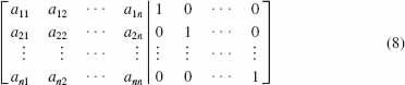
we then apply a succession or row operations on (8) until we have transformed it into a new matrix,
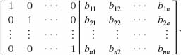
where the matrix to the left of the vertical bar is now In. The inverse of A is
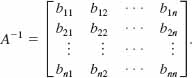
This procedure is illustrated in the next two examples.
EXAMPLE 5 Using Elementary Row Operations
Use elementary row operations to find A -1 for
![]()
Solution We begin by forming the matrix
![]()
The idea is to transform the matrix to the left of the vertical line into the matrix I2. Now,
Because I2 now appears to the left of the vertical line, we conclude that the matrix to the right of this line is
![]()
This result can now be checked by the previous method or by multiplication. Choosing the latter procedure, we see that AA-1 and A-1A are, in turn,
EXAMPLE 6 Example 3 Revisited
Use elementary row operations to find A -1 for the matrix in Example 3.
Solution We have
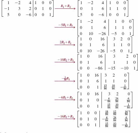
As before, we see that
In conclusion, we note that if an n × n matrix A cannot be transformed into the multiplicative identity In by elementary row operations, then A is necessarily singular. If, at some point in the applications of the elementary row operations, we find a row of zeros in the matrix on the left side of the vertical line, then the matrix A is singular. For example, from
![]()
we see that it is now impossible, using only row operations, to obtain I2 to the left of the vertical line. Thus the 2 × 2 matrix
![]()
is singular.
9.4 Exercises Answers to selected odd-numbered problems begin on page ANS-22.
In Problems 1 and 2, verify that the matrix B is the inverse of the matrix A.
1. ![]()
2. 
In Problems 3-14, use Method 1 of this section to find the multiplicative inverse, if it exists, of the given matrix. Assume all variables are nonzero.
3. ![]()
4. ![]()
5. ![]()
6. ![]()
7. 
8. ![]()
9. 
10. 
11. 
12. 
13. 
14. 
In Problems 15-26, use Method 2 of this section to find the multiplicative inverse, if it exists, of the given matrix.
15. ![]()
16. ![]()
17. ![]()
18. ![]()
19. ![]()
20. ![]()
21. 
22. 
23. 
24. 
25. 
26. 
27. If ![]() what is A?
what is A?
28. Find the inverse of ![]()
In Problems 29 and 30, suppose ![]() . Verify the given property of the inverse by computing the left and right members of the given equality.
. Verify the given property of the inverse by computing the left and right members of the given equality.
29. (A–1)–1 = A
30. (AB)–1 = B -1A–1
For Discussion
31. Let
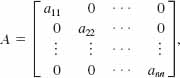
where aij ≠ 0, i = 1, 2,…, n. What is A -1?
32. Use the result in Problem 31 to find A-1 for the matrix
33. If ![]() , then find x and y.
, then find x and y.
34. If A–1 is given by (5), verify that A–1A = I2.
35. Let A, B, and C be n × n matrices, where A is nonsingular. Discuss: How would you prove that if AB = AC, then B = C?
36. In Problem 29, we saw that (A–1)–1 = A for a nonsingular 2 × 2 matrix. This result is true for any nonsingular n × n matrix. Discuss: How would you prove this general result?
37. In Problem 30, we saw that (AB)–1 = B 1A–1for two nonsingular 2 × 2 matrices. This result is true for any two nonsingular n × n matrices. Discuss: How would you prove this general result?
38. Let A be a 2 × 2 matrix for which det A × 0. Show that det A–1 = 1/det A. This result is true for any nonsingular n × n matrix.
9.5 Linear Systems: Augmented Matrices
![]() Introduction In Example 2 of Section 8.1, we solved the system of linear equations
Introduction In Example 2 of Section 8.1, we solved the system of linear equations
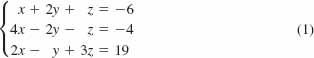
by finding an equivalent system in triangular form:
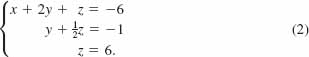
The system (2) was obtained from system (1) by a series of operations on the equations that changed the coefficients of the variables and the constants on the right-hand side of the equality. Throughout this procedure the variables acted as “placeholders.” Therefore, these same calculations can be simplified by performing operations on the rows of the matrix
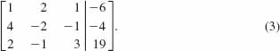
![]() Augmented Matrices The matrix in (3) is called the augmented matrix of the system (1) and consists of the coefficient matrix
Augmented Matrices The matrix in (3) is called the augmented matrix of the system (1) and consists of the coefficient matrix
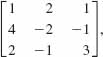
augmented by adding a column whose entries consist of the constant terms of the system. The vertical line in an augmented matrix enables us to distinguish the coefficients of the variables in the system from the constant terms of the system.
When the elimination operations introduced in Section 8.1 are applied to a system of equations, we obtain an equivalent system of equations. These elimination operations are analogous to the elementary row operations that we discussed in the preceding section. When elementary row operations are applied to an augmented matrix, the result is the augmented matrix of an equivalent system. For this reason, the original matrix and the resulting matrix are said to be row equivalent. The procedure of carrying out elementary row operations on a matrix to obtain a row equivalent matrix is called row reduction.
![]() Gaussian Elimination To solve a system such as (1) using an augmented matrix, we will use either Gaussian elimination or Gauss-Jordan elimination. In the Gaussian elimination, we row reduce the augmented matrix of the system until we arrive at a row equivalent augmented matrix in row echelon form.
Gaussian Elimination To solve a system such as (1) using an augmented matrix, we will use either Gaussian elimination or Gauss-Jordan elimination. In the Gaussian elimination, we row reduce the augmented matrix of the system until we arrive at a row equivalent augmented matrix in row echelon form.
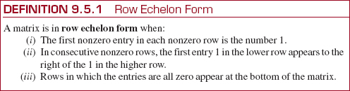
EXAMPLE 1 Row Echelon Form
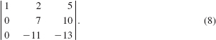
The two augmented matrices
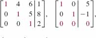
are in row echelon form, whereas the matrix
is not in row echelon form.
As we see in Example 1, the row echelon form of an augmented matrix is roughly a triangular form with zero entries below a diagonal consisting of 1's.
To reduce an augmented matrix to row echelon form we use the same elementary row operations introduced in Section 9.4:
Ri↔Rj: Interchange the ith row with the j th row.
kRi: Multiply the ith row by a constant k.
kRi + Rj: Multiply the i th row by k and add to the j th equation.
EXAMPLE 2 System (1) Revisited
Solve the system (1) using Gaussian elimination.
Solution We begin by using the first row to introduce 0's below the 1 in the first column:

Since this final augmented matrix is in row echelon form (and corresponds to the system (2)) we have, in fact, solved the original system. The last row of the matrix implies that z = 6. The remaining variables are determined by back-substitution. Substituting z = 6 back into the equation corresponding to the second row of the matrix yields y = -5. Finally, substituting y = -5 and z = 6 into the equation corresponding to the first row yields x = -2. Thus the solution is x = -2, y = -5, z = 6.
In Example 2, note that we repeated, in order, the elementary row operations corresponding to the operations that were performed on the equations when we solved this system by elimination (see Example 2 in Section 8.1). Thus we are not doing anything new here. We have simply removed the variables and the equality signs from the equations and are relying on the format of the matrix to keep things in order.
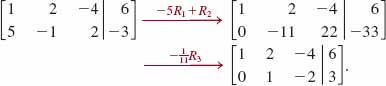
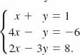
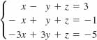
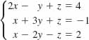
EXAMPLE 3 Using Gaussian Elimination
Use Gaussian elimination to solve the system
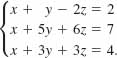
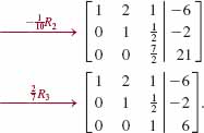
Solution We form the augmented matrix of the system and perform elementary row operations until we obtain a row echelon form:
The last augmented matrix is in row echelon form and corresponds to the system
From the last equation we see immediately that ![]() , From the second equation we then obtain
, From the second equation we then obtain ![]() . And finally, the first equation gives us
. And finally, the first equation gives us ![]() . Therefore,
. Therefore, ![]() is the solution of the system.
is the solution of the system.
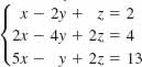
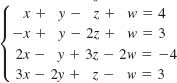
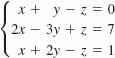
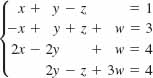
EXAMPLE 4 Using Gaussian Elimination
Use Gaussian elimination to solve the system
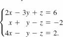
Solution We use elementary row operations:
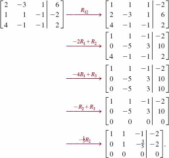
The last matrix is the augmented matrix of the system
![]()
Solving for x and y in terms of z, we find
![]()
Thus the given system is consistent, but the equations are dependent. There are infinitely many solutions of the systems obtained by assigning arbitrary real values to z. If we denote z by α, the solutions of the system consist of all x, y, and z defined by ![]() , respectively, where a represents any real number.
, respectively, where a represents any real number.
The technique discussed in this section is also applicable to systems of m linear equations in n unknowns. In the following example, we consider a system of two equations in three unknowns.
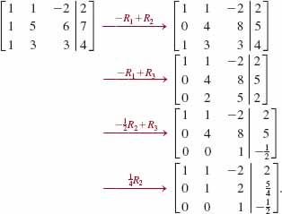
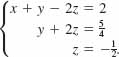
EXAMPLE 5 Using Gaussian Elimination
Use Gaussian elimination to solve the system
![]()
Solution We have
From the last matrix in row echelon form, we find
![]()
Using the second equation to eliminate y from the first, we then obtain
![]()
As in Example 4, we may assign any value to z. Hence the solutions of the system are defined by ![]() , where α is any real number.
, where α is any real number.
![]() Gauss-Jordan Elimination In the Gauss-Jordan elimination method, the elementary row operations are continued until we obtain an augmented matrix that is in reduced row echelon form. A reduced row echelon matrix has the three properties (i)-(iii) in Definition 9.5.1, but in addition:
Gauss-Jordan Elimination In the Gauss-Jordan elimination method, the elementary row operations are continued until we obtain an augmented matrix that is in reduced row echelon form. A reduced row echelon matrix has the three properties (i)-(iii) in Definition 9.5.1, but in addition:
(iv) A column containing first entry 1 has zeros everywhere else.
EXAMPLE 6 Reduced Row Echelon Form
(a) The augmented matrices
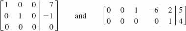
are in reduced row echelon form. You should verify that the four criteria for this form are satisfied.
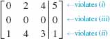
(b) We have seen in Example 1 that the augmented matrix
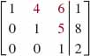
is in row echelon form. However, the augmented matrix is not in reduced row echelon form because the remaining entries (indicated in red) in the columns that contain a leading entry 1 are not all zero.
In should be noted that in Gaussian elimination, we stop when we have obtained an augmented matrix in row echelon form. In other words, by using different sequences of row operations, we may arrive at different row echelon forms. This method then requires the use of back substitution. In Gauss-Jordan elimination, we stop when we have obtained the augmented matrix in reduced row echelon form. Any sequence of row operations will lead to the same augmented matrix in reduced row echelon form. This method does not require back substitution; the solution of the system will be apparent by inspection of the final matrix. In terms of the equations of the original system our goal is to simply make the coefficient of the first variable in the first equation* equal to 1 and then use multiples of that equation to eliminate the variable from other equations. The process is repeated on the other variables.
EXAMPLE 7 Example 3 Revisited
In solving the system in Example 3,
we stopped when we obtained a row echelon form. We now start with the last matrix in Example 3. Since the first entries in the second and third rows are 1's, we must, in turn, make the remaining entries in the second and third columns 0's:
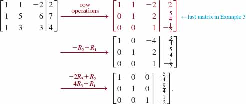
The last matrix is in reduced row echelon form. Bearing in mind what the matrix means in terms of equations, we see immediately that the solution is ![]() .
.
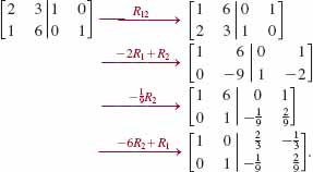
EXAMPLE 8 Inconsistent System
Use Gauss-Jordan elimination to solve the system
Solution In the process of applying Gauss-Jordan elimination to the matrix of the system, we stop at
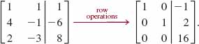
The third row of the last matrix means 0x + 0y = 16 (or 0 = 16). Since no numbers x and y can satisfy this equation, we conclude that the system has no solution, that is, it is inconsistent.
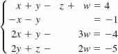
EXAMPLE 9 Balancing a Chemical Equation
Balance the chemical equation C2H6 + O2 → CO2 + H2O.
Solution We seek positive integers x, y, z, and w so that the balanced equation is
![]()
Because the number of atoms of each element must be the same on each side of the last equation, we obtain a homogeneous system of three equations in four variables:
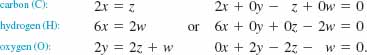
![]() See Section 8.1.
See Section 8.1.
Since the last system is homogeneous it must be consistent.
Using elementary row operations, we find
and so a solution of the system is ![]() . In this case a must be a positive integer chosen in such a manner so that x, y, z, and w are positive integers. To accomplish this we pick α = 6. This gives x = 2, y = 7, z = 4, and w = 6. The balanced equation is then
. In this case a must be a positive integer chosen in such a manner so that x, y, z, and w are positive integers. To accomplish this we pick α = 6. This gives x = 2, y = 7, z = 4, and w = 6. The balanced equation is then
2C2H6 + 7O2 → 4CO2 + 6H2O.
9.5 Exercises Answers to selected odd-numbered problems begin on page ANS-23.
In Problems 1-4, write the coefficient matrix and the augmented matrix of the given system of equations.
1. 
2. 
3. 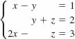
4. 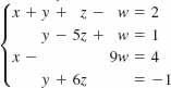
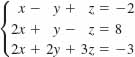
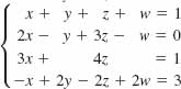
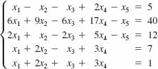
In Problems 5-32, solve the given system, or show that no solution exists. Use Gaussian elimination or Gauss-Jordan elimination as directed by your instructor.
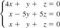
5. ![]()
6. ![]()
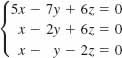
7. ![]()
8. ![]()
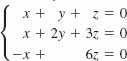
9. 
10. 
11. 
12. 
13. 
14. 
15. 
16. 
17. 
18. 
19. 
20. 
21. 
22. 
23. 
24. 
25. 
26. 
27. 
28. 
29. ![]()
30. ![]()
31. 
32. ![]()
In Problems 33-38, use the procedure illustrated in Example 9 to balance the given chemical equation.
33. Na + H2O → NaOH + H2
34. KClO3 → KCl + O2
35. Fe3O4 + C → Fe + CO
36. C5H8 + O2 → CO2 1 H2O
37. Cu + HNO3 → Cu(NO 3)2 + H2O + NO
38. Ca3(PO4)2 + H3PO4 → Ca(H2PO4)2
39. Find a quadratic function f (x) = ax2 + bx + c whose graph passes through the three points (1, 8), (-1, -4), and (3, 4).
40. Find coefficients a, b, and c such that (1, 1, -1), (-2, -3, 3), and ![]() are solutions of the equation ax + by + cz = 1.
are solutions of the equation ax + by + cz = 1.
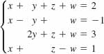
41. Find x, y, z, and w such that
![]()
42. Write a system of equations corresponding to the augmented matrix
Miscellaneous Applications
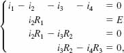
43. Current in a Circuit The currents i1, i2, and i3 in the electrical network shown in FIGURE 9.5.1 can be shown to satisfy the system of linear equations
![]()
where R1, R2, R3, and E are positive constants. Use Gauss-Jordan elimination to solve the system when R1 = 10, R2 = 20, R3 = 10, and E = 12.
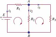
FIGURE 9.5.1 Network in Problem 43
44. Counting the A, B, C's A company has 100 employees divided into three categories A, B, and C. As the following table shows, each employee makes a different contribution to a retirement fund. Following negotiation of a new contract, the monthly contribution of the employees increases by the indicated percentage. The total monthly contribution of $4450 by all employees then increases to $5270 because of the new contract. Use the concept of an augmented matrix to determine the number of employees in each category.

Calculator/CAS Problems
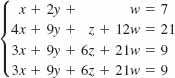
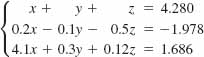
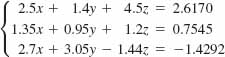
In Problems 45-48, use a calculator or CAS to solve the given system.
45. 
46. 
47. 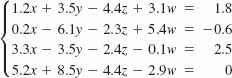
48. 
9.6 Linear Systems: Matrix Inverses
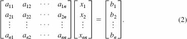
![]() Introduction In this and the next section we will confine our attention to solving only linear systems with n equations and n variables x1, x2,…, xn:
Introduction In this and the next section we will confine our attention to solving only linear systems with n equations and n variables x1, x2,…, xn:
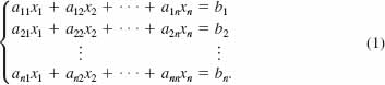
If the determinant of the coefficients of the variables in the system (1) is denoted by
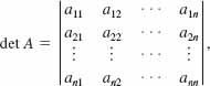
then in this and Section 9.7 we solve linear systems such as (1) under the further assumption that det A ≠ 0.
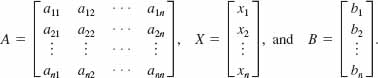
![]() Matrix Form of (1) Using matrix multiplication and equality, we can write the linear system (1) as the matrix equation
Matrix Form of (1) Using matrix multiplication and equality, we can write the linear system (1) as the matrix equation
In other words, if A is the coefficient matrix for the system (1), then we can write (1) as
![]()
where
EXAMPLE 1 Matrix Form of a Linear System
The system of equations
![]()
can be written as
![]()
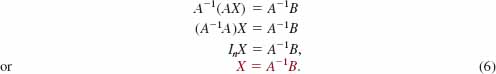
![]() Matrix Solution If the inverse of the coefficient matrix A exists, we can solve system (3) by multiplying both sides of the equation by A-1:
Matrix Solution If the inverse of the coefficient matrix A exists, we can solve system (3) by multiplying both sides of the equation by A-1:
EXAMPLE 2 Example 1 Revisited
Use the inverse of a matrix to solve the system in (4).
Solution Because the determinant of the coefficient matrix A is not zero,
![]()
and the matrix A has a multiplicative inverse, and so
![]()
By either of the two methods of Section 9.4, we find that
![]()
Hence, it follows from (6) that the solution of (4) is
Therefore, ![]() is the solution of the given system.
is the solution of the given system.
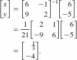
EXAMPLE 3 Using a Matrix Inverse
Use the inverse of a matrix to solve the system
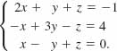
Solution The given system can be written as
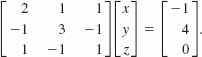
Because the determinant of the coefficient matrix is det A = 2 ≠ 0 its inverse is found to be
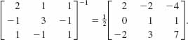
Thus by (6) we have
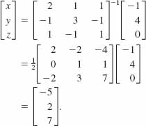
The solution of the system is given by x =-5, y = 2, z = 7.
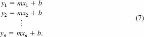
![]() Least Squares Line—Revisited In Section 4.8 we saw that if we try to fit a line y = mx + b to a set of data points (x1, y1), (x2, y2),…, (xn, yn), then m and b must satisfy a system of linear equations
Least Squares Line—Revisited In Section 4.8 we saw that if we try to fit a line y = mx + b to a set of data points (x1, y1), (x2, y2),…, (xn, yn), then m and b must satisfy a system of linear equations
In terms of matrices system (7) is Y = AX, where

We define the solution of (7) to be the values of m and b that minimize the sum of square errors
![]()
and correspondingly y = mx + b is called the least squares line or the line of best fit for the data. The slope m and constant b are defined by cumbersome quotients of sums given in (5) of Section 4.8. These formulas, derived using calculus, are actually solutions of a linear system in the two variables m and b:
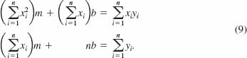
The foregoing system can be written in a special manner using matrices:
![]()
where A, X, and Y are defined in (8). SinceAis an n × 2matrix and its transpose AT is a 2 × n matrix, the dimension of the product AT A is 2 × 2. Moreover, unless the data points all lie on the same vertical line, the matrix ATA is nonsingular. Thus, (10) has the unique solution
![]()
We say that X is the least squares solution of the overdetermined system (7).
The next example is Example 2 of Section 4.8, but worked this time using matrices.
EXAMPLE 4 Example 2, Section 4.8
Find the least squares line for the data (1, 1), (2, 2), (3, 4), (4, 6), (5, 5).
Solution The linear equation y = mx + b and the data (1, 1), (2, 2), (3, 4), (4, 6), (5, 5) lead to the overdetermined system
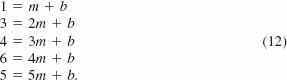
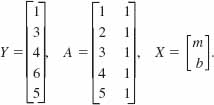
Written as a matrix equation Y = AX, (12) enables us to make the identifications
Now
![]()
and so (11) gives

From the entries in the last matrix, the least squares solution of (12) is m = 1.1 and b = 0.5 and the least squares line is y = 1.1x + 0.5.
NOTES FROM THE CLASSROOM
In conclusion, we note that not all consistent n × n systems of linear equations can be solved by the method outlined in Examples 2 and 3. This procedure obviously fails for those linear systems in which the coefficient matrix A has no inverse, that is, for those systems for which det A = 0. However, when det A ≠ 0, it can be proved that an n × n system of linear equations has a unique solution.
9.6 Exercises Answers to selected odd-numbered problems begin on page ANS-23.
In Problems 1-18, write each linear system in the form AX = B. Then use an inverse matrix to solve the system.
1. ![]()
2. ![]()
3. ![]()
4. ![]()
5. ![]()
6. ![]()
7. ![]()
8. ![]()
9. 
10. 
11. 
12. 
13. 
14. 
15. 
16. 
17. 
18. 
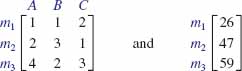
In Problems 19-22, use an inverse matrix to solve the system
![]()
for the given matrix ![]() .
.
19. ![]()
20. ![]()
21. ![]()
22. ![]()
In Problems 23-28, proceed as in Example 4 and find the least squares line for the given data.
23. (2, 1), (3, 2), (4, 3), (5, 2)
24. (0, -1), (1, 3), (2, 5), (3, 7)
25. (1, 1), (2, 1.5), (3, 3), (4, 4.5), (5, 5)
26. (0, 0), (2, 1.5), (3, 3), (4, 4.5), (5, 5)
27. (0, 2), (1, 3), (2, 5), (3, 5), (4, 9), (5, 8), (6, 10)
28. (1, 2), (2, 2.5), (3, 1), (4, 1.5), (5, 2), (6, 3.2), (7, 5)
Miscellaneous Applications
In Problems 29-31, use an inverse matrix to solve the problem.
29. Playing with Numbers The sum of three numbers is 12. The second number is 1 more than 3 times the first, and the third number is 1 less than 2 times the second. Find the numbers.
30. Counting the A, B, C's A company manufactures three products A, B, and C from materials m1, m2, and m3. The two matrices
represent, in turn, the number of units of material used in the construction of each product and the number of units of each type of material used in a specific week. Find
![]()
where x, y, and z are, respectively, the number of products that are manufactured in that particular week.
31. Probing the Depths This problem shows how the depth of an ocean and the speed of sound in water can be measured by a procedure known as echo sounding. Suppose that an oceanographic vessel emits sonar signals and that the arrival times of the signals reflected from the flat ocean floor are recorded at two trailing sonobuoys. See FIGURE 9.6.1. Using the relation distance = rate × time, we see from the figure that 2l1 = vt1 and 2l2 = vt2, where v is the speed of sound in water, t1 and t2 are the arrival times of the signals at the two sonobuoys, and l1 and l2 are the indicated distances.
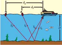
FIGURE 9.6.1 Echo sounding procedure in Problem 31
(a) Show that the speed of sound in water v and ocean depth D satisfy the matrix equation
![]()
[Hint: Use the Pythagorean theorem to relate l1, d1, and D, and l2, d2, and D.]
(b) Solve the matrix equation in part (a) to obtain formulas for v and D in terms of the measurable quantities d1, d2, t1, and t2.
(c) The sonobuoys, trailing at 1000 and 2000 m, record the arrival times of the reflected signals at 1.4 and 1.8 seconds, respectively. Find the depth of the ocean and the speed of sound in water.
9.7 Linear Systems: Determinants
![]() Introduction In some circumstances, we can use determinants to solve systems of n linear equations in n variables.
Introduction In some circumstances, we can use determinants to solve systems of n linear equations in n variables.
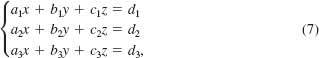
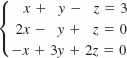
Suppose the linear equations in the system
![]()
are independent. If we multiply the first equation by b2 and the second by –b1, we obtain
![]()
In the last form of the system we can eliminate the y-variable by adding the two equations. Solving for x gives
![]()
Similarly, by eliminating the x-variable, we find
![]()
If we denote three 2 × 2 matrices by
![]()
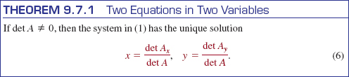
where A is the matrix of the coefficients in (1), then the numerators and the common denominator in (2) and (3) can be written as second-order determinants:
![]()
The determinants det Ax and det Ay in (5) are, in turn, obtained from det A by replacing the x-coefficients and then the y-coefficients by the constant terms c1 and c2 of system (1).
With this notation we can summarize the discussion in a compact fashion.
EXAMPLE 1 Using (6)
Solve the system
![]()
Solution Since
![]()
it follows that the system has a unique solution. Continuing, we find
![]()
From (6) the solution is given by
![]()
In like manner, the solution (6) can be extended to larger systems of linear equations. In particular, for a system of three equations in three variables,
and the determinants analogous to those in (5) are
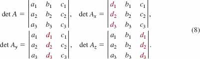
![]() Indicated by the red d1, d2, and d3 in (8).
Indicated by the red d1, d2, and d3 in (8).
As in (5), the three determinants det Ax, det Ay, and det Az are obtained from the determinant det A of the coefficients of the system, by replacing the x-, y-, and z-coefficients, respectively, by the constant terms dl, d2, and d3 in each of the three linear equations in the system (7). The solution of the system (7) that is analogous to (6) is given next.
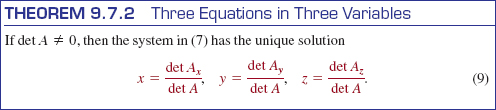
The solutions in (6) and (9) are special cases of a more general method known as Cramer's rule, named after the Swiss mathematician Gabriel Cramer (1704-1752), who was the first to publish these results.
EXAMPLE 2 Using Cramer's Rule
Solve the system
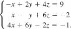
Solution We evaluate the four 3 × 3 determinants in (9) using cofactor expansion. We begin by finding the value of the determinant of the coefficients in the system:
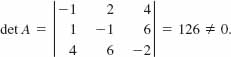
The fact that this determinant is nonzero is sufficient to indicate that the system is consistent and has a unique solution. Continuing, we find
From (9), the solution of the system is then
![]()
When the determinant of the coefficients of the variables in a linear system is 0, Cramer's rule cannot be used. As we see in the next example, this does not mean the system has no solution.
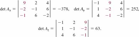
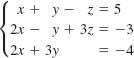
EXAMPLE 3 Consistent System
For the system
![]()
we see that
![]()
Although we cannot apply (6), the method of elimination would show us that the system is consistent but that the equations in the system are dependent.
The equations in (9) can be extended to systems of n linear equations in n variables x1, x2,…, xn. For the system (1) in Section 9.6, Cramer's rule is
![]()
provided det A ≠ 0. As a practical matter, Cramer's rule is seldom used on systems with a large number of equations simply because evaluating the determinants becomes a Herculean task. For large systems, the methods discussed in Section 9.5 are the most efficient means of solution.
9.7 Exercises Answers to selected odd-numbered problems begin on page ANS-23.
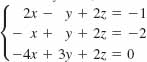
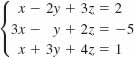
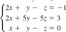
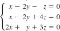
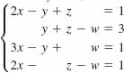
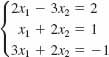
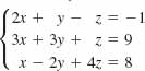
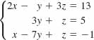
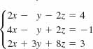
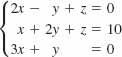
In Problems 1-14, use Cramer's rule to solve the given system.
1. ![]()
2. ![]()
3. ![]()
4. ![]()
5. ![]()
6. ![]()
7. 
8. 
9. 
10. 
11. 
12. 
13. 
14. 
Miscellaneous Applications
15. Take Your Vitamin s The U.S. recommended daily allowance (U.S. RDA), in percent of vitamin content per ounce of food groups X, Y, and Z, is given in the following table.
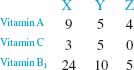
Use Cramer's rule to determine how many ounces of each food group one must consume each day in order to get 100% of the daily recommended allowance of vitamin A, 30% of the daily recommended allowance of vitamin B1, and 200% of the daily recommended allowance of vitamin C. Let x, y, and z be the number of ounces of food groups X, Y, and Z, respectively.
9.8 Cryptography
![]() Introduction The word cryptography is a combination of two Greek words: crypto, which means “hidden” or “secret,” and grapho, which means “writing.” Cryptography then is the study of making “secret writings” or codes. In this section we will consider a system of encoding and decoding messages that requires both the sender of the message and the receiver of the message to know
Introduction The word cryptography is a combination of two Greek words: crypto, which means “hidden” or “secret,” and grapho, which means “writing.” Cryptography then is the study of making “secret writings” or codes. In this section we will consider a system of encoding and decoding messages that requires both the sender of the message and the receiver of the message to know
a specified rule of correspondence between a set of symbols (such as letters of the alphabet and punctuation marks from which messages are composed) and a set of integers, and
a specified nonsingular matrix A.
![]() Encoding/Decoding A natural correspondence between the first 27 nonnegative integers and the letters of the alphabet and a blank space (to separate words) is given by
Encoding/Decoding A natural correspondence between the first 27 nonnegative integers and the letters of the alphabet and a blank space (to separate words) is given by
![]()
Using the correspondence (1) the numerical equivalent of the message
SEND THE DOCUMENT TODAY
is
![]()
The sender of the message will encode it by means of a nonsingular matrix A and the receiver of the encoded message will decode it by means of the (unique) matrix A-1. The matrix A is called the encoding matrix and A-1 is called the decoding matrix. The numerical message (2) is now written as a matrix M. Since there are 23 symbols in the message we need a matrix that will hold a minimum of 24 entries (an m × n matrix has mn entries). We choose to write (2) as the 3 × 8 matrix
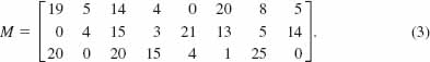
Note that the last entry (a38) in the matrix M has been simply padded with a space represented by the number 0. Of course we could have written the message (2) as a 6 × 4 matrix or a 4 × 6 matrix but that would require a larger encoding matrix. The choice of a 3 × 8 matrix allows us to encode the message by means of a 3 × 3 matrix. The size of the matrices used is a concern only when the encoding and decoding are done by hand rather than by a computer.
The encoding matrix A is chosen, or rather, constructed, so that
A is nonsingular,
A has only integer entries, and
A-1 has only integer entries.
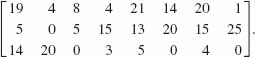
The last criterion is not particularly difficult to accomplish. We need only select the integer entries of A in such a manner so that det A = ±1. For a 2 × 2 or a 3 × 3 matrix we can then find A-1 by the formulas in (5) and (6) of Section 9.4. If A has integer entries, then all the cofactors A11, A12, and so on are also integers. For the discussion on hand we choose
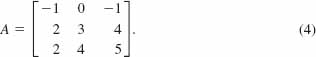
You should verify that det A = –1.
The original message is encoded by premultiplying the message matrix M by the encoding matrix A; that is, the message is sent as the matrix B = AM. Using (3) and (4) the encoded message is
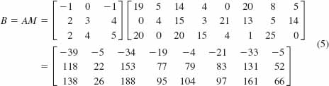
You should try to imagine the difficulty of decoding the last matrix in (5) without knowledge of A. But the receiver of the message B knows A and its inverse and so the decoding is the straightforward computation of premultiplying B by the decoding matrix A-1:
![]()
For the matrix (4) we find from (6) of Section 9.4 that
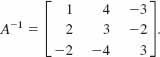
Thus from (6) the decoded message is
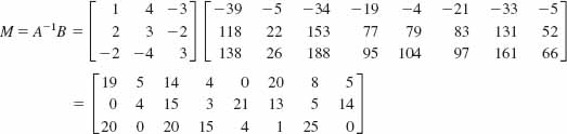
or
![]()
By also knowing the original correspondence (1), the receiver translates the numbers into
SEND_THE_DOCUMENT_TODAY_,
where we have emphasized the blank spaces by dashes.
![]() Observations Several observations are in order. The correspondence or mapping (1) is one of many such correspondences that can be set up between the letters of the alphabet (we could even include punctuation symbols such as the comma and period) and integers. Using the 26 letters of the alphabet and the blank space we can set up 27! of these kinds of correspondences. (See Section 10.6.) Furthermore, we could have used a 2 × 2 matrix to encode (2). The size of the message matrix Mwould then have to be at least 2 × 12 in order to contain the 23 entries of the message. For example, if the encoding and message matrices are, respectively,
Observations Several observations are in order. The correspondence or mapping (1) is one of many such correspondences that can be set up between the letters of the alphabet (we could even include punctuation symbols such as the comma and period) and integers. Using the 26 letters of the alphabet and the blank space we can set up 27! of these kinds of correspondences. (See Section 10.6.) Furthermore, we could have used a 2 × 2 matrix to encode (2). The size of the message matrix Mwould then have to be at least 2 × 12 in order to contain the 23 entries of the message. For example, if the encoding and message matrices are, respectively,
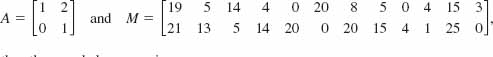
then the encoded message is
![]()
Using the decoding matrix ![]() we obtain as before
we obtain as before
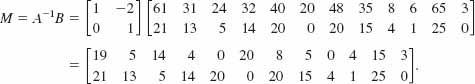
There is no particular reason why the numerical message (2) has to be broken down as rows (1 × 8 row vectors) as in the matrix (3). Alternatively, (2) could be broken down as columns (3 × 1 column vectors) as shown in the matrix
Finally, it may be desirable to send the encoded message as letters of the alphabet rather than as numbers. In Problem 13 in Exercises 9.8 we show how to transmit SEND THE DOCUMENT TODAY encoded as
OVTHWFUVJVRWYBWYCZZNWPZL.
9.8 Exercises Answers to selected odd-numbered problems begin on page ANS-23.
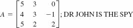
In Problems 1-6, (a) use the matrix A and the correspondence (1) to encode the given message, and (b) verify your work by decoding the encoded message.
1. ![]()
2. ![]()
3. ![]()
4. 
5. 
6. 
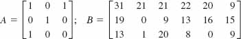
In Problems 7-10, use the matrix A and the correspondence (1) to decode the given message.
7. ![]()
8. ![]()
9. 
10. 
11. Using the correspondence (1), a message M was encoded using a 2 × 2 matrix to give
![]()
Decode the message if its first two letters are DA and its last two letters are AY.
12. (a) Using the correspondence
![]()
find the numerical equivalent of the message
BUY ALL AVAILABLE STOCK AT MARKET.
(b) Encode the message by postmultiplying the message matrix M by
(c) Verify your work by decoding the encoded message in part (b).
13. Consider the matrices A and B defined in (4) and (5), respectively.
(a) Rewrite B as the matrix B' using integers modulo 27.
(b) Verify that the encoded message to be sent in letters is
OVTHWFUVJVRWYBWYCZZNWPZL.
(c) Decode the encoded message by computing A-lB' and rewriting the result using integers modulo 27.
![]()
A. True/False__________________________________________________
In Problems 1-12, answer true or false.
1. If A is a square matrix such that det A = 0, then A-1 does not exist.___
2. If A is a 3 × 3 matrix for which the cofactor ![]() , then det A = 0.___
, then det A = 0.___
3. If A, B, and C are matrices such that AB = AC, then B = C.___
4. Every square matrix A has an inverse matrix A-1.__________
5. If AB = C and if C has two columns, then B necessarily has two columns.____
6. The matrix 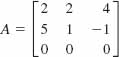 is singular._______
7. If A and B are 2 × 2 singular matrices, then A + B is also singular.____
8. If A is a nonsingular matrix such that A2 = A, then det A = 1.______
9. If ![]() and ad = bc, then A-1 does not exist._____
and ad = bc, then A-1 does not exist._____
10. ![]()
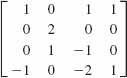
11. The augmented matrix  is in reduced row echelon form._____
12. If a ≠ 0 and b ≠ 0, then
![]()
B. Fill in the Blanks_____________________________________________
In Problems 1-12, fill in the blanks.
1. If A has 3 rows and 4 columns and B has 4 rows and 6 columns, then the dimension of the product AB is____________.
2. If A has dimension m × n and B has dimension n × m, then the dimension of AB is________and the dimension of BA is________.
3. If A = (aij)4×5, where aij = 2i2 – j3, then the entry in the third row and second column is________.
4. Suppose A is a square matrix and B is the matrix formed by interchanging the first two columns in A. If det A = 12, then det B = ________.
5. ![]() and det A = 2, then x =________.
and det A = 2, then x =________.
6. If 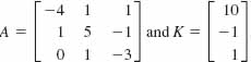 , the number λ for which AK = λ K is________.
7. If ![]() and A + B = O, then B = ________.
and A + B = O, then B = ________.
8. If A = (aij)4×4, where aij = 0, i ≠ j, then det A = ________.
9. An example of a 2 × 2 matrix A ≠ I2 such that A2 = I2 is________.
10. The minor determinant M22of the matrix 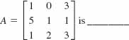
11. The cofactor of 5 in the matrix 
12. If A and B are n × n matrices whose corresponding entries in the third column are the same, then det(A – B) = 0 because________.
C. Review Exercises_____________________________________________
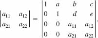
1. Solve for the unknowns:![]() .
.
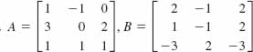
2. For
![]()
find A + B and (-2)A + 3B.
3. The currents in an electrical network satisfy the system of equations
where R1 R2, R3, and E are positive constants. Use Cramer's rule to show that
![]()
4. Two n × n matrices A and B are said to anticommute if AB = –BA. Find two different pairs of 2 × 2 matrices that anticommute.
5. Find all cofactors Aij of the entries aij for the matrix
6. Show that if A is a nonsingular matrix for which det A = 1, then A -1 = adj A.
In Problems 7-10, suppose
and det A = 2. Determine the value of the given determinant.
7. det (4A)
8. 
9. 
10. 
In Problems 11 and 12, evaluate the determinant of the given matrix.
11. 
12. 
In Problems 13 and 14, use Theorems 9.4.1 and 9.4.2 to find A -1 for the given matrix.
13. ![]()
14. 
In Problems 15 and 16, use elementary row operations to find A -1 for the given matrix.
15. ![]()
16. 
In Problems 17 and 18, write the system as an augmented matrix. Solve the system by Gaussian elimination.
17. ![]()
18. 
In Problems 19 and 20, write the system as an augmented matrix. Solve the system by Gauss-Jordan elimination.
19. 
20. ![]()
In Problems 21 and 22, use an inverse matrix to solve the given system.
21. 
22. ![]()
In Problems 23 and 24, use Cramer's rule to solve the given system.
23. ![]()
24. 
In Problems 25 and 26, expand the given determinant by cofactors other than those of the first row.
25. 
26. 
27. Find the values of x for which the matrix
is nonsingular. Find A–1.
28. Prove that the matrix
is singular.
In Problems 29-40, suppose
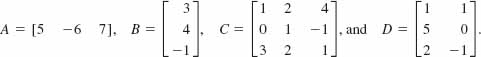
Find the indicated matrix if it is defined.
29. A – BT
30. –3C
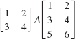
31. A(2B)
32. 5BA
33. AD
34. DA
35. (BA)C
36. (AB)C
37. CTB
38. BTD
39. C-1(BA)
40. C2
41. Show that there exists no 2 × 2 matrix with real entries such that
![]()
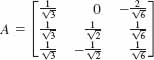
42. Show that AT = A-1 for the matrix
43. Let A and B be 2 × 2 matrices. Is it true, in general, that
(AB)2 = A2B2
44. Show that if ![]() , then A2 = A-1, where A2 = AA.
, then A2 = A-1, where A2 = AA.
45. Show that
46. Suppose that A is the 2 × 2 matrix
![]()
(a) Show that the matrix A satisfies the equation A2 – A – 2I2 = O, where O is the 2 × 2 zero matrix.
(b) Use the equation in part (a) to show that A3 = 3A + 2I2 and A4 = 5A + 6I2. [Hint: Multiply the equation by A.]
(c) Use the right-hand side of the appropriate equation in part (b) to compute A3and A4.
47. Show that if X1 and X2 are solutions of the homogeneous system of linear equations AX = O, then X1 + X2 is also a solution.
48. Use the matrix ![]() to encode the message
to encode the message
SATELLITE LAUNCHED ON FRI.
Use the correspondence given in (1) of Section 9.8.
* We can always interchange equations so that the first equation contains the variable x1.
* For integers a and b, we write a = b (mod 27) if b is the remainder (0 ≤ b < 27) when a is divided by 27. For example, 33 = 6 (mod 27), 28 = 1 (mod 27), and so on. Negative integers are handled in the following manner. Since 27 = 0 (mod 27) then, for example, 25 + 2 = 0 (mod 27) so that –25 = 2 (mod 27) and –2 = 25 (mod 27). Also, –30 = 24 (mod 27) since 30 + 24 = 54 = 0 (mod 27).