6 Small-World Wireless Mesh Networks

Search in book...
Toggle Font Controls
Create new playlist

Name your new playlist

Playlist description (optional)
Sign In

Email address

Password

Forgot Password?

or

Continue with Facebook

Continue with Google
Sign Up

Full Name

Email address

Confirm Email Address

Password

or

Continue with Facebook

Continue with Google

Chapter 6
Small-World Wireless Mesh Networks

The concept of small-world characteristics offers many benefits when applied to wireless multi-hop relaying networks to minimize the end-to-end hop distance and delay in transmission of data packets. Wireless mesh networks (WMNs), which are a type of multi-hop relaying network, find many applications in civilian as well as tactical communication networks for the following benefits: (i) multi-hop relaying, (ii) easy network deployment and reconfiguration, (iii) low cost of operation, and (iv) improved network reliability and robustness. Small-world characteristics incorporate significant performance benefits such as lower average path length (APL), lower end-to-end delay in data transmission, better load balancing in the network, and improved quality of service. This chapter presents characteristics of small-world wireless mesh networks (SWWMNs), which is followed by a detailed discussion on existing small-world creation strategies in the context of SWWMNs. A comparative study is also presented on the existing small-world models and their applicability in SWWMNs. A set of open research problems are also included at the end of the chapter.

6.1 Introduction

WMNs [17] are distributed wireless networks that use wireless medium for communication over partial or full mesh topology with multi-hop relaying. WMNs typically have three types of nodes: mesh router, mesh client, and gateway mesh router. A typical WMN, with all node types, is shown in Figure 6.1. In a WMN, mesh routers are either static nodes or nodes with limited mobility; therefore, the router nodes act as access points. Mesh routers perform all the routing functionalities and network maintenance operations in a WMN.

Mesh clients, on the other hand, are end user devices which are typically mobile in WMNs. Any electronic equipment with wireless multi-hop relaying capability such as laptops, tablets, mobile phones, and personal digital assistants can be considered as mesh client. A mesh client is connected by means of multi-hop relaying with other mesh clients or mesh routers. Gateway mesh routers have a backbone-wired interface by which they associate with other wired or existing wireless networks.

Figure 6.1. An example wireless mesh network

Mesh routers are equipped with wireless network radios built on the same or different wireless access technologies [17]. Other than routing functions for a gateway or repeater, mesh routers are proficient in other functional capabilities for carrying out mesh networking. The multi-hop relaying capability of mesh routers allows them to efficiently provide coverage in broader geographical areas. Therefore, with the same amount of power consumption, mesh routers can provide service to larger areas than the conventional single-hop wireless routers. To communicate with the existing backbone-wired infrastructure/Internet, mesh routers route packets through gateway mesh routers.

ThereexistthreemainWMNarchitectures: (i) infrastructure/backbone WMNs, (ii) client WMNs, and (iii) hybrid WMNs. An infrastructure/backbone WMN forms a backbone network through a gateway mesh router. The gateway router helps the infrastructure WMN to connect to the Internet and helps mesh clients to communicate with existing wireless and wired networks. A client WMN is formed by the multi-hop relaying among the mesh clients. Mesh clients in a client WMN communicate among themselves without the involvement of mesh routers. Therefore, all tasks of self-configuration, network maintenance, and network routing are carried out by the mesh clients in the network. As a node in a client WMN has to execute the role of mesh client as well as mesh router, the functional complexity of the mesh node in the client WMN is increased. A hybrid WMN, on the other hand, comprises an infrastructure WMN and a client WMN. Therefore, a hybrid WMN consists of two tiers of WMNs. In the lower tier, data packets are delivered using multi-hop relaying among mesh clients, thus forming client WMNs. The upper tier is composed of an infrastructure WMN which helps the lower tier mesh nodes to connect with the Internet or existing wired/wireless networks. Mesh clients can communicate to the Internet by multi-hop relaying with the gateway mesh routers. Figure 6.2 illustrates the architecture of a hybrid WMN.

An example of a hybrid wireless mesh network.

Figure 6.2. Architecture of a hybrid wireless mesh network

Mobile ad hoc networks (MANETs) are another type of infrastructure-less multi-hop relaying network [12]. Here, mobile nodes need to perform self-configuration and all the routing functionalities for relaying packets in the network. Moreover, network topology and connectivity are dependent on the mobility of the nodes in a MANET. Therefore, the end-to-end network connectivity may not be reliable in MANETs all the time. However, WMNs are infrastructure-based networks which deploy partially mobile- or fixed topology– based multi-hop relaying. Therefore, the end-to-end network connectivity in WMNs is improved over MANETs, and mobility impact on the network is reduced significantly.

The end-to-end throughput in finite real-world WMNs can be increased by minimizing the averaged end-to-end hop distance (EHD) between source nodes (SNs) and destination nodes (DNs). In wireless environments, hop-distance is a function of the spatial separation among the network nodes. Hence, distance between two nodes can be varied in the network. If EHDs between SN-DN pairs can be minimized, the end-to-end transmission delay in the network can also be reduced. Furthermore, network reliability, quality of service, and network throughput also can be improved. One way to minimize the EHD in finite real-world WMNs is to incorporate the small-world characteristics.

6.1.1 The Small-World Characteristics

The small-world characteristics were first observed by Stanley Milgram [64] in his 1967 experiment in social psychology. The experiment showed that people are connected by means of a small number of intermediate acquaintances (i.e., five to nine hops with a median value of 6), popularly known as the notion of six degrees of separation. The conclusion drawn by the experiment is proved to be beneficial in several fields of study.

Watts and Strogatz first observed the small-world characteristics in a scientific study of various networks such as neural networks of Caenorhabditis elegans, power-grid networks of the western United States, and the collaboration networks of film actors [6]. The study of real-world networks revealed that the small-world networks exhibit low to moderate average clustering coefficient (ACC) as well as low APL. ACC is the fraction of connecting neighbor nodes averaged over the entire network. APL measures the mean distance between an SN and a DN averaged over all SNs and DNs in the network. A detailed discussion on ACC and APL can be found in Section 2.4.

6.1.2 Small-World Wireless Mesh Networks

In a WMN, mesh nodes (i.e., mesh clients as well as mesh routers) are interconnected by means of wireless multi-hop relaying. Transmission power in WMNs is a critical parameter because allocation of higher transmission power in the mesh nodes introduces severe interference among the neighbor nodes, and as a result, throughput of the network decreases. Hence, mesh nodes use minimal transmission power to minimize the effect of interference in the network. However, the value of APL is typically high in WMNs.

The throughput of a WMN comprising n number of mesh nodes is λ(n), where $λ (n) \leq n W r (n) / \overline{L}$ $λ (n) \leq n W r (n) / \overline{L}$ . Here, r(n) is the radio range of each WMN router, W is the transmission rate in bps, and $\overline{L}$ $\overline{L}$ is the APL in terms of number of EHD averaged over the network. Therefore, network throughput can be enhanced by improving transmission rate, increasing radio range of router nodes, or reducing APL of the WMN. However, enhancing the bandwidth of operation (i.e., enhancing W) is too expensive. Moreover, increasing r(n) for each node is not a suitable solution because it requires more power and introduces more interference in the network. Therefore, reducing the value of $\overline{L}$ $\overline{L}$ is a more practical approach to enhance the throughput of a WMN.

Therefore, to achieve low APL value, the EHD between SN and DN averaged over the WMN has to be reduced. By implementing a handful number of long-ranged links (LLs) among distant node pairs (i.e., non-neighbors) in the existing network, EHD between SN and DN can be reduced. An SWWMN can be formed either by rewiring of existing links or by the addition of new LLs in a WMN. In the following sections, a set of LL implementation strategies to reduce APL are discussed.

6.2 Classification of Small-World Wireless Mesh Networks

The small-world characteristic implementation gives low APL in finite real-world WMNs; therefore, performance enhancement in terms of network throughput can be achieved along with lower end-to-end transmission delay.

Network traffic fairness, on the other hand, can be achieved by distributing the traffic load throughout all nodes in the network. In WMNs, the nodes at the center of the network face high traffic load. However, mesh nodes which are located at the boundary of the network face less traffic congestion due to the spatial traffic distribution within a WMN. By careful implementation of LLs among the distant node pairs in the WMNs, traffic load can be distributed uniformly across the WMN nodes. Therefore, traffic fairness in the network operation of an SWWMN can also be improved.

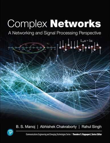
The existing models on implementation of small-world characteristics in WMNs can broadly be classified in two categories: persistent and non-persistent LL creation strategies. Small-world implementation by persistent LL creation in WMNs is one of the possibilities by which APL of the finite real-world WMNs can be minimized. Once established, persistent LLs do not change their locations during the data packet transmission. However, non-persistent LLs change their locations in SWWMNs. Figure 6.3 shows the classification chart of existing models to realize SWWMNs.

Creation of persistent LLs again can be subdivided in random LL creation and deterministic LL creation. In persistent random LL creation strategies, LLs are created to transform a regular network to a small-world network based on certain random decision or strategy. LLs can be created either by randomly rewiring the existing normal links (NLs) [6], [94], or by adding a few LLs randomly or deterministically in the network. Random LL addition in an SWWMN is performed by pure random addition [68], contact-based LL addition [94], Euclidean distance– based LL addition [69], based on antenna metrics [119], [120], [121], or based on gateway mesh routers [122], [95]. Moreover, random LL addition can also be realized by implementing genetic algorithm [123] or cooperative routing [124].

LLs can also be deterministically created in a regular network to optimize certain network characteristics when persistent deterministic LL creation is concerned. A set of deterministic strategies are LL addition to minimize APL (MinAPL), to minimize average edge length (MinAEL), to maximize betweenness centrality (MaxBC), to maximize closeness centrality (MaxCC), to maximize closeness centrality disparity (MaxCCD), and sequential deterministic LL addition (SDLA) [72], [77].

In the case of non-persistent LL creation, data-mule-based [125] and load-aware non-persistent LL creation [126] techniques are considered in this chapter.

6.3 Creation of Random Long-Ranged Links

In random LL creation, a set of LLs are created, based on either pure probability or depending on some metric (e.g., Euclidean distance), in a regular network to transform a regular network into a small-world network. Random LL creation is further divided into (i) rewiring the NLs and (ii) addition of new LLs.

The classification of the major approaches involved in small-world wireless mesh networks.

The root is Classification of SWWMNs. It branches into two: Persistent and Non-Persistent. Persistent further has two divisions: Random and Deterministic. Random is divided into Rewiring and Addition. Addition is classified into the following: Pure Random, Euclidean Distance, Metrics of Antenna, Algorithmic, and Gateway Router. The following are under Metrics of Antenna: Power Control, Beam-Forming, and Both. Algorithmic is further divided into Contact based, GA based, and SWCR based. Gateway Router is classified into Single Gateway that contains RAS, GAS, and GAGS; and Multi-Gateway that contains M-GAS and LM-GAS. Deterministic is classified into two: Exhaustive Search which contains MinAPL, MinAEL, MaxBC, and MaxCC; and Heuristics Approach which contains MaxCCD and SDLA. The divisions under Deterministic are separately enclosed within a block that is tagged See Chapter 5. Non-persistent is classified into Data Mule and Load-Aware Routing.

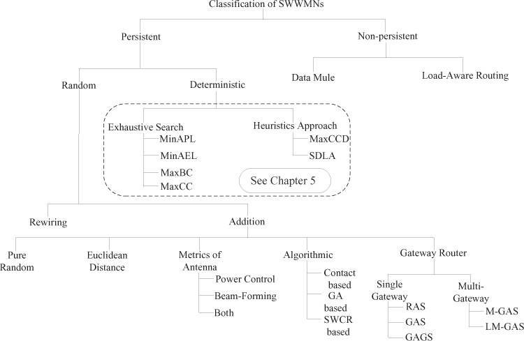
Figure 6.3. Classification of major approaches in small-world wireless mesh networks (SWWMNs)

6.3.1 Random LL Creation by Rewiring the Normal Links

Rewiring is a persistent LL creation procedure in which some of the existing NLs are rewired to other nodes. Thus, in rewiring, a small number of NLs of an existing regular lattice can be rewired based on some probability p where 0 ≤ p ≤ 1 [6].

Rewiring of NLs is one of the procedures by which a regular network can be transformed to a small-world network. In the process of rewiring, a regular network (with probability p = 0) can be converted to completely random network (p = 1). In the transformation from regular to a complete random network, the small-world characteristics can be observed for 0 < p < 1. This situation is depicted in Figure 6.4.

Figure 6.4(a) shows a WMN grid composed of mesh routers which are connected to form a regular network with NLs (rewiring probability p = 0). Hence, the average neighbor degree is moderate for the network, whereas APL is large, as can be seen in Figure 6.4(a). Now, a handful of NLs can be removed and reconnected with probability 0 < p < 1 to certain distant nodes (bidirectional solid line in Figure 6.4(b)) as LLs. Therefore, APL is reduced in the WMN as the end-to-end distances among the distant nodes in the network are reduced. In this process, by rewiring a small number of existing NLs, lower value of APL can be achieved. However, ACC is kept nearly unchanged compared to the a regular network. Therefore, the small-world characteristics in a regular network can be realized by rewiring a set of the existing NLs to some distant nodes. However, when NLs are rewired with rewiring probability p = 1 in a WMN, as shown in Figure 6.4(c), the regular grid becomes a random WMN which has the lowest value of APL; however, the ACC value is also reduced because neighbor nodes may not be connected when a random network is concerned. Hence, in order to realize an SWWMN, a limited number of LLs is sufficient, as depicted in Figure 6.4(b).

A regular grid network, small-world network, and random network are illustrated.

On the top, the components used in the networks along with their symbols are listed as follows: a Mesh Router, a dotted line for a Normal Link (NL), and a bi-directional arrow Long-Ranged Link (LL). The three figures are alphabetically labeled and placed side-by-side. All have a 4 cross 4 grid, with a Mesh Router placed over the vertices of the grid. Each router is connected to every other router around it by dotted lines. This is the regular grid network depicted in figure a. In figure b, the dotted lines between the router at the following positions are removed: (2, 2) and (2, 3), (3, 1) and (3, 2), and (3, 3) and (3, 4). The following routers are connected with bi-directional arrowheads: (2, 2) and (3, 4), (3, 1) and (1, 3), and (3, 3) and (2, 1). This is the small-world network. Figure c shows the random network. Here, the dotted lines connecting the routers at the following router positions from the initial grid are removed: (1, 1) and (1, 2), (2, 2) and (2, 3), (3, 3) and (3, 4), (4, 1) and (4, 2), and (4, 2) and (4, 3). The following routers are connected with bi-directional arrowheads: (1, 1) and (4, 2), (1, 2) and (4, 4), (1, 3) and (3, 1), (1, 4) and (3, 2), (2, 2) and (2, 4), (2, 3) and (4,1), and (2, 4) and (3, 3).

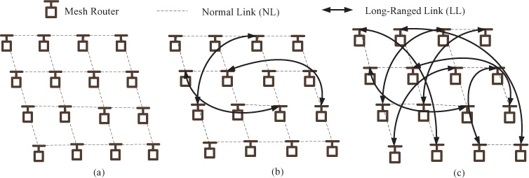
Figure 6.4. Rewiring in a regular grid lattice: (a) A regular grid network with rewiring probability p = 0, (b) the grid is converted to a small-world network with rewiring probability 0 < p < 1, and (c) with p = 1, the small-world network is transformed to a random network.

The rewiring strategy can also be realized in the context of multi-hop wireless network settings [94]. Wireless networks are spatial networks with highly clustered topologies. In this model, a node is selected randomly, and then a link from one of its neighbors is unlinked in order to rewire to another random node in the network. The rewiring strategy, hence, is similar to the rewiring strategy discussed previously. It can be observed that 0.2% to 20% rewiring of NLs drastically reduces the APL value of the wireless multi-hop networks. However, further rewiring does not reduce the APL value in the similar rate due to the LL saturation in the network.

Advantages and Disadvantages of Rewiring-Based SWWMNs

Rewiring-based LL creation strategy imposes the following advantages. (i) Rewiring requires only local information to rewire an existing NL. Therefore, information overhead can be reduced. (ii) The time complexity, with rewiring, to create an LL in an N-node network is only $𝒪 (1)$ $? (1)$ .

However, rewiring in the context of WMNs introduces many difficulties. (i) Rewiring in the wireless environment requires some additional information to steer the antenna from the earlier direction (i.e., from the direction of previous NL connecting node) to the direction of the new node where the LL has to be created. Moreover, (ii) NLs in a typical WMN are created by omnidirectional antennas; therefore, it is difficult to create an LL by rewiring an existing NL in the specified direction when only omnidirectional antennas are present in the network.

6.3.2 Random LL Creation by Addition of New Links

Since rewiring of existing links is difficult in a broadcast wireless network, small-world characteristics can also be realized by adding some new LLs in the existing regular network. In this strategy, the existing NLs are unaltered by LL addition process. Instead, addition of LLs is preferred. Most of the existing models on small-world networks are based on the concept of addition of new LLs in the regular network [121], [122], [68], [69], [94], [95], [119], [120], [123], [124]. The technique of addition of LLs to achieve a small-world network is again subcategorized into several strategies. In the following, various types of LL addition strategies are presented.

6.4 Small-World Based on Pure Random Link Addition

Pure random LL addition refers to a method where new LLs are added among distant node pairs based on probability p [68]. It can be observed from the earlier discussion that the rewiring strategy involved removing one end of an NL and connecting it to another long-distance node to create an LL in the network. This creation of persistent LL transits its phase continuously [6] with the rewiring of NLs in the network.¹ However, in pure random LL addition strategy, new LLs are added without removing the existing NLs from the network. Hence, the phase transition does not take place in this strategy because the existing NLs are not removed from the network. Furthermore, the operational overhead in pure random addition technique is lower compared to the rewiring of the existing NLs.

Advantage and Disadvantage of Pure Random Link Addition–Based SWWMNs

The advantage of the pure random LL addition strategy is that the strategy is less complex in its implementation. However, the main disadvantage of this strategy is its failure to deterministically reduce the APL of the network.

6.5 Small-World Based on Euclidean Distance

LLs can also be created based on the measured lattice distance (i.e., Euclidean distance). The Euclidean distance–based LL addition model is also known as Kleinberg’s model because the model was first proposed by Jon Kleinberg [69]. Euclidean distance or Manhattan distance can be measured between two points in a grid-like path as the absolute difference in their coordinates. The probability of LL addition was based on the expression d(u, υ)^−α/∑_v _≠_u d(u, υ)^−α, where d(u, υ) is the Euclidean distance between node u and node υ (see Figure 6.5), which is averaged over all node distances (minimum distance of a node pair ≥ 2) in the network to get the normalized probability of addition of LL between two nodes. Here, α is the clustering exponent, which takes the value equal to the dimension of the network (i.e., for 1-D network, α = 1 and so on). It can be observed that for a 2-D grid network, α = 2 gives the lowest value of APL [79].

A 2D grid network for the addition of new LLs.

Figure 6.5. A 2-D grid network for addition of new LLs with the probability d(u, υ)^−α/∑_v _≠_u d(u, υ)^−α

Advantages and Disadvantages of Euclidean Distance–Based SWWMNs

The advantages of the Euclidean distance–based LL addition strategy or the Klein-berg’s model [69] are as follows. (i) The probability of LL addition is based on fewer parameters such as the Euclidean distance between the node pairs and the clustering exponent α of the network, and (ii) the implementation does not require global information, as it is based on the decentralized algorithm (a detailed discussion on decentralized algorithm can be found in Section 4.10.1).

However, there are some disadvantages of Kleinberg’s model when SWWMNs are concerned. (i) The geographical/Euclidean information is essential in Kleinberg’s model for network creation, which may not be available in many real-world situations. Therefore, in such cases the model has only theoretical significance. Moreover, (ii) in mobile networks, the distance between nodes may vary dynamically, and thus, the link addition probability cannot be estimated appropriately. If nodes remain less mobile or static in the context of a WMN, location information can be retrieved prior to the addition of LLs in WMN. However, for highly mobile WMNs, implementation of Kleinberg’s small-world network model is challenging.

6.6 Realization of Small-World Networks Based on Antenna Metrics

Mesh nodes (i.e., mesh clients and mesh routers) in WMNs communicate with the help of radio interfaces. Antenna elements can be used as the transceivers in the radio environment to transport data packets among nodes in a WMN. Mesh nodes transmit data packets in the direction of the radiation of the antenna element.

Two important metrics of an antenna element are the transmission power and the beamformer. By controlling transmission power of the WMN antenna or by changing the direction or the range of the beamformer, new long-ranged connections can be established in the SWWMNs. A set of existing models that suggest creation of LLs by controlling antenna metrics are described in the following.

6.6.1 LL Addition Based on Transmission Power

The transmission power of some nodes in WMNs can be enhanced to communicate with long-distance nodes. By enhancing the transmission range of the sender nodes, LLs can be created in existing wireless networks. However, enhancement of the transmission range results in increased interference in WMNs. Therefore, highly directional antennas are required to reduce the amount of interference in the network.

An uneven probabilistic flooding technique can be deployed to minimize the APL value of the wireless multi-hop network [119]. A few wireless nodes are assumed as the strong nodes in the networks. Strong nodes are equipped with two transceivers with different radio ranges. The transmission power of one of the transceivers of the strong node is increased to nearly double the other transceivers, and it is dedicated for long-distance communication in the network. The distance covered by the strong node, over an LL, is assumed to be twice the ordinary wireless nodes of the networks. The ordinary nodes are equipped with two receivers (to receive data simultaneously from other ordinary as well as strong nodes) and one transmitter. Moreover, the strong nodes can be assigned higher probability of data transmission than the ordinary nodes in the networks.

Advantages and Disadvantages of Transmission Power–Based SWWMNs

The advantages of the uneven probabilistic flooding–based strategy are that (i) the value of APL can be reduced as the number of strong nodes is increased, and hence, (ii) the delay in the networks also decreases.

The main disadvantages of the approach are (i) higher cost of network installation and (ii) the large-sized message overhead for the probabilistic message flooding algorithm.

6.6.2 LL Addition Based on Randomized Beamforming

A randomized beamforming strategy can also be deployed, with the distributive algorithm, to achieve SWWMNs [121]. In the process of beamforming, the radio frequency energy is concentrated by the antenna elements in a particular direction of radiation in the wireless environment to form a major lobe. Hence, with beamformer, long-distance communication is possible in the wireless environment using the same power as the omnidirectional antenna. Some random nodes can be selected based on the fraction of probability p and equipped with long-range directional antennas.

The directional beamformers are capable of providing coverage in a particular spatial direction. As the directional beam is concentrated in one particular direction of communication, it covers more distance than the omnidirectional antenna, which caters its beam in all the directions of its vicinity. Hence, the directional antennas can be used for long-range transmission in SWWMNs. In randomized beamforming [121], APL can be reduced by implementing directional beamformer to some randomly selected nodes. The LL implementation strategy is depicted in Figure 6.6.

It is assumed, in the randomized beamforming strategy, that the nodes are connected by means of omnidirectional transceivers. Moreover, the random nodes with directional antennas are equipped with omnidirectional antennas for reception.

A metric called wireless flow betweenness (WFB) is suggested, in the randomized beamforming strategy, for better performance of the randomized algorithm where random nodes are selected for LL addition. WFB measures the presence of a node in constructing a communication link between node pairs in a wireless network. WFB is same as the betweenness centrality (BC), as can be found in Section 3.3.1. Hence, high value of betweenness indicates that the node is present in most of the paths in the network. Figure 6.7 shows an example where WFB is demonstrated. Since node A in Figure 6.7 is present in most of the established communication paths among the remaining node pairs, A can be considered as one of the LL creating nodes to achieve lower APL. However, node B and node C are not present in most of the communication paths in the network. Therefore, they do not have as high a WFB as A in the network of Figure 6.7.

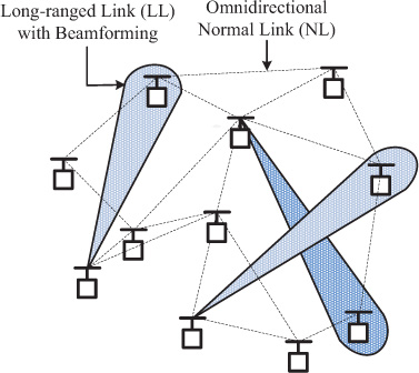
An illustration of the creation of Long-ranged link by directional beamforming.

Figure 6.6. Long-ranged link creation by directional beamforming

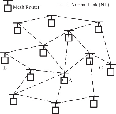
An illustration of a wireless flow betweenness is displayed.

Figure 6.7. An example of wireless flow betweenness [121]

The measure of WFB of the network can give a precise measure of flow betweenness centrality (FBC), which measures the packet transmission rate through the central node (e.g., node A in Figure 6.7). Hence, APL value can be greatly reduced when new LLs are connected with the central nodes with higher values of WFB.

Advantages and Disadvantages of Randomized Beamforming-Based SWWMNs

The major advantages of the randomized beamforming strategy are the following. (i) With the same power as the NLs, beamforming along with traffic flow information helps in long-distance communication in the network. (ii) With the introduction of WFB, identification of central nodes improves overall path length reduction in the context of data transmission between distant nodes.

The randomized beamforming strategy imposes some difficulties too. (i) The mechanism to reduce the interference in the network, with beamformers as LLs, is not clearly addressed. (ii) The randomized beamforming strategy does not consider the situation when a data packet has to be transmitted to a node which is outside the covered region of the major lobe.

6.6.3 LL Addition Based on Transmission Power and Beamforming

Directional beamforming along with transmission power control is another approach by which small-world properties can be realized in the context of WMNs [120]. In this strategy, power control of the antenna is implemented with zero-forcing beamforming (ZFB) to realize small-world wireless networks. The zero-forcing or null-steering is a spatial signal processing technique by which multiple transmitting antennas can mitigate the ill effect of interference in the wireless network environment.

It can be assumed in the directional beamforming strategy that the channel of signal transmission follows a power-law model based on the path-loss exponent η, expressed as P_r = P_t d^−η where P_t and P_r are the transmitted and received power, respectively, for distance d [120]. It is also assumed that each node has the same number of adjacent nodes which are positioned at the same distance from each other. Furthermore, the physical carrier sensing range of each wireless node in the multi-tier network is assumed to be twice the transmission range.

To implement the power control algorithm, the multi-tier network is divided into several large hexagons which are again partitioned into seven small hexagons. When the center node sends data packets for tier d, all the (d − 1) tiers (as all the tiers are assumed to be situated at unit distance from each other) avoid any communication by sensing the transmission of data packets for tier d. Hence, for longer sensing range (and the transmission range as well), more wireless nodes remain inactive by carrier sensing, and the transmission opportunity (TXOP) is reduced for the center node in the network lattice [120]. Therefore, in spite of reduced EHD, end-to-end throughput of the network lattice degrades.

To achieve higher end-to-end throughput, it can be assumed that the center nodes of the multi-tier lattice are equipped with multiple directional antennas. Moreover, it can be observed that when power control and ZFB are used together, the end-to-end throughput of the network is increased. Two-directional antennas are used for the center nodes, and the capacity of the center nodes is increased significantly due to the ZFB [120]. Furthermore, the center node may nullify the delay in the transmission by accepting the weighted average of the transmitted signals.

Advantage and Disadvantage of Transmission Power and Beamforming–Based SWWMNs

The advantage of LL creation based on both transmission power and beamforming is that the network discussed above can be implemented as a multi-tier relaying networks. However, the main disadvantages of the strategy are that (i) most of the traffic is concentrated in the center node, so load balancing becomes an issue in the network, and (ii) due to the TXOP setting, many nodes remain inactive, which in turn reduce the end-to-end throughput of the network.

6.7 Algorithmic Approaches to Create Small-World Wireless Mesh Networks

There exist a few LL creation strategies, in SWWMNs, based on the following algorithms: (i) contact-based [94], (ii) genetic algorithm-based [123], and (iii) cooperative routing–based [124] LL addition strategies. In the following, each of the LL addition strategies is discussed.

6.7.1 Contact-Based LL Creation

A contact-based approach can be used for the discovery of distant nodes to create an LL in wireless multi-hop network. Here, contact means that a node inquires its neighbors for resources to reach a distant DN by creating certain shortcuts in the network. Shortcuts can be created either by rewiring existing NLs with probability p or by adding new LLs in the wireless networks [94].

To create LLs in wireless medium, in general, either the transmission range or the receiver sensitivity of the existing omnidirectional antennas can be enhanced in the context of each wireless router node. In contact-based SWWMNs, each router node has two transmission radios: one radio with lower transmission range to communicate with the nearest one-hop router nodes, and the other transmission radio with higher transmission range, which can create an LL with a distant node in the network.

In the contact-based approach, an LL is created by rewiring a random NL with the probability p to other distant node, or an LL is randomly added between a node pair based on the end-to-end distance d, where d is varied from [2, r] hops. The maximum value of r can be the diameter (D) of the SWWMNs. It can be seen from the simulation observations, on various network topologies such as normal, random, grid, and skewed, that creation (by rewiring or addition) of small fractions of LLs (0.2% to 20%) with a specified diameter (r/D ∼ 25% to 40%) can reduce the APL of the network while the value of ACC remains almost same as the original network [94].

Advantage and Disadvantage of Contact-Based SWWMNs

The advantage of the contact-based LL creation approach is that the LL creation strategy, based on either rewiring or addition, reduces the network APL. However, the disadvantage of this approach is that the realization of rewiring-based LLs is very difficult in SWWMNs.

6.7.2 Genetic Algorithm–Based LL Addition

A genetic algorithm (GA)–based strategy can also be implemented to identify an LL connecting location and its optimal length to minimize the APL value. GA can be used to determine the probable locations of LLs in the network. An important factor in this approach is the set of random nodes, chosen from a grid network, to add LLs. The chosen random nodes are equipped with two transceivers having different radio transmission ranges. One transceiver is used as an NL for neighborhood communications, and the other is treated as the LL transceiver for transmission of data packets to the distant nodes. It can be seen, through simulation experiments, that when an LL is connected between two mesh nodes with an EHD of at least six hops, APL is reduced noticeably [123].

Advantage and Disadvantage of GA-Based SWWMNs

The advantage of GA-based LL creation is that the number as well as the length of LLs can be determined with this approach. However, the disadvantage is that the interference issue in creating LLs in the wireless medium is not considered.

6.7.3 Small-World Cooperative Routing–Based LL Addition

Cooperative routing protocol–based LL addition can also be used to get SWWMNs [124]. Cooperative communication, or cooperative diversity, is a data transmission mechanism in which the cooperative node relays the data packets to the nearest node of the DN.Hence, the relaying node must be equipped with multiple transmitters to transmit its own data and relay its neighbor’s data as well. In small-world-based cooperative routing (SWCR), cooperative nodes are used to create LLs between SNs and DNs to bring down APL in the ad hoc network, keeping ACC nearly unchanged. Figure 6.8 shows a schematic of the cooperative diversity scheme to realize small-world network character.

In SWCR, the EHD is measured by the greedy routing mechanism, which works on the basis of topological information of the DN. In Figure 6.8, i₁, j₁, and k₁ are the LL connecting nodes which relay the data packets of SN, u to the DN, through node i₂. As the cooperative link r₁ between SN and i₁ has the shortest Euclidean distance, the first LL is considered between u and i₁. Here, LL is created based on the relation given by Kleinberg’s model [79]. The link r₂ between i₁ and i₂ is the cooperative link which is created by i₁, based on availability of the topological information and greedy routing algorithm.

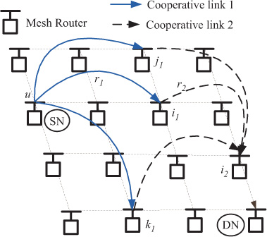
An illustration of a small-world based cooperative communications network.

Figure 6.8. Small-world based cooperative communications

The SWCR-based small-world WMN approach implements both physical as well as logical links. As a result of that, the value of APL is greatly reduced. It can be seen that the implementation of SWCR model brings the value of APL nearly $𝒪 [N$ $? [N$ log $N / (M q)]$ $N / (M q)]$ , where N is the number of nodes in the network, q is the parameter which has value in the range of 1 < q < log N, and M is the number of cooperative router nodes. The minimum APL is attained when the EHD between an SN-DN pair becomes $𝒪 [($ $? [($ log $N)^{2} / q]$ $N)^{2} / q]$ .

In WMN, the choice of cooperative nodes requires prior knowledge about the topology of the network and the location of the mesh routers that can be used as cooperative nodes in the WMN. Each node in SWCR-based routing stores the locations of all shortcut nodes in a routing table and then, based on that topological knowledge, nodes in the network execute routing. However, locations of the router nodes are mostly static in a WMN; therefore, cooperative routing may be implemented in a WMN to achieve lower APL.

Advantage and Disadvantage of SWCR-Based SWWMNs

The advantage of SWCR-based LL creation is that overall APL can be improved meaningfully by the introduction of logical and physical LLs. The disadvantage of this approach is its need for global knowledge to identify the cooperative nodes to create LLs.

6.8 Gateway-Router-Centric Small-World Network Formation

A typical WMN comprises mobile client nodes, mesh router nodes, and single or multiple gateway router nodes. Client nodes in a WMN communicate to each other through fixed mesh routers in a multi-hop fashion, whereas the mesh routers communicate to the Internet or infrastructure networks with the help of the gateway routers. In the gateway-router-centric approach, a small number of wireless routers are equipped with long-ranged radio interfaces to achieve small-world characteristics in WMNs. However, the LL addition strategies consider gateway-APL (G-APL) for deciding the positions of LLs in the network. Since all WMN routers in most WMN deployments communicate through the WMN gateway, a slightly different variant of APL, G-APL, which estimates the average hop length between the WMN routers and the gateway, is used for performance evaluation (see Section 2.4.3 for more details about G-APL). As the gateway routers are responsible for the connectivity with the Internet or other infrastructure-based wireless networks, the EHD between WMN routers and the WMN gateway can be reduced in the wireless network by introducing a few long-range connections between WMN routers. Note that the gateway router is excluded from the LL addition because LL addition at the gateway will transform the entire network to a collection of WLANs instead of an SWWMN. Therefore, the actual APL value from the client nodes to the Internet in an SWWMN is (G-APL + 1) hops.

Based on the number of gateway routers present in a WMN, LL addition strategies can be divided into the following: (i) single gateway-router-based and (ii) multi-gateway-routers-based LL addition strategies.

6.8.1 Single Gateway-Router-Based LL Addition

Single gateway-router-based LL addition strategy for WMNs [95] is employed through the constrained small-world architecture for wireless network (C-SWAWN) model. C-SWAWN architecture considers key constraints such as limited transmission ranges for NLs (R_S) and LLs (R_L), and limited number of LLs per node (K_LL), and can be represented as C-SWAWN(R_S, R_L, K_LL). Figure 6.9 shows an example of SWWMN where all LLs are added by the C-SWAWN approach.

The LLs in an SWWMN with a single gateway router can be added based on three strategies [95]: (i) random LL addition strategy (RAS), (ii) gateway-aware LL addition strategy (GAS), and (iii) gateway-aware greedy LL addition strategy (GAGS).

Random LL Addition Strategy-Based SWWMNs

In RAS, a pair of WMN router nodes, say p and q, are chosen randomly to add an LL in the network. However, RAS checks basic constraints such as R_S, R_L, and K_LL before adding an LL between p and q. Note that the Euclidean distance between nodes p and q should lie between R_S and R_L, and both the nodes should have at least one unassigned long-ranged radio to accommodate an LL. Algorithm 6.1 lists the LL addition approach with RAS.

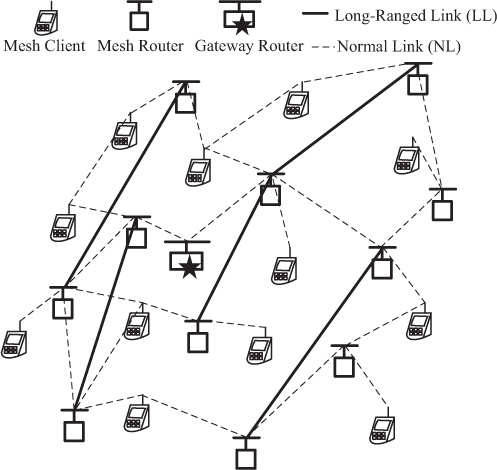
An illustration of a single gateway-router-based SWWMN creation.

Figure 6.9. Single gateway-router-based SWWMN creation

To add i^th LL in a WMN, Algorithm 6.1 randomly selects a router node pair and then checks for the required constraints (lines 2–3). If both router nodes satisfy the constraints, the i^th LL is added between them and K_LL values for both the nodes are decremented to one (lines 4–5). On the other hand, if creation of an LL is not possible between the selected router nodes, the algorithm again searches for another random router node pair to add the i^th LL (lines 6–8). This LL addition procedure continues until N_LL LLs are added in the WMN.

Time Complexity of RAS

The time complexity of RAS to add N_LL LLs in an SWWMN can be evaluated as follows. Consider that there are N number of fixed router nodes which can be used to add N_LL LLs in the SWWMN. To add an LL in the network, Algorithm 6.1 randomly searches for a node pair in $𝒪 (1)$ $? (1)$ time (Line 2). The rest of the algorithm (lines 3–9) can also be executed in $𝒪 (1)$ $? (1)$ time. Hence, to add N_LL LLs, RAS is $𝒪 (N_{L L})$ $? (N_{L L})$ time complex.

Gateway-Aware LL Addition Strategy–Based SWWMNs

In GAS, the G-APL of the SWWMN can be improved. GAS exploits the technique adopted in RAS (see Section 6.8.1) including an additional constraint |d(i) − d(j)| ≥ Δ_h. Here, d(i) represents the distance of node i from the gateway router in the WMN. Δ_h is a controllable parameter, with minimum value of 2, which captures the minimum shortest hop distance between the gateway router and the node pair that are selected for adding a new LL. In GAS, LLs are added in the SWWMN until either the limit of maximum number of LLs (N_LL) is reached or the network becomes saturated with N_sat number of LLs with respect to the network controlling parameters R_L, K_LL, and Δ_h. GAS-based single gateway-router-aware LL addition strategy is depicted in Algorithm 6.2.

Algorithm 6.1 Random LL Addition Strategy (RAS)

Require:

$𝒢 = (𝒱_{1}, 𝒱_{2}, G_{R}, ℰ)$ $? = (?_{1}, ?_{2}, G_{R}, ℰ)$ — Graphical representation of a wireless mesh network with $ℰ$ $ℰ$ links

$𝒱_{1}$ $?_{1}$ — Number of mesh routers in $𝒢$ $?$

$𝒱_{2}$ $?_{2}$ — Number of mesh clients in $𝒢$ $?$

G_R — Number of gateway mesh routers in $𝒢$ $?$

N_LL — Total number of long-ranged links (LLs) to be added in $𝒢$ $?$

R_S — Maximum range of short-ranged radios

R_L — Maximum range of long-ranged radios

K_LL — Maximum number of LLs that can be accommodated by each node in $𝒱_{1}$ $?_{1}$

K_LL_(i,j) — K_LL values for node i and j

ED_{(i, j)} — Euclidean distance between nodes i and j

Initialization: R_S, R_L, K_LL

1: for i = 1 → N_LL do

2: Randomly select two nodes p_i and q_i ∀ p_i, q_i ∈ $𝒱_{1}$ $?_{1}$

3: if R_S ≤ ED_{(p_i, q_i)} ≤ R_L & K_LL_{(p_i, q_i)} ≠ 0 then

4: Add i^th LL between p_i and q_i

5: Decrement K_LL values for p_i and q_i

6: else

7: go to 2

8: end if

9: Update network graph G

10: end for

LL addition in an SWWMN with Algorithm 6.2 executes as follows. First, two router nodes, say p and q, are randomly selected to add i^th LL (Line 2). However, nodes p and q should satisfy all required constraints (line 3). If all constraints are satisfied, then the i^th LL is added and corresponding K_LL values are updated for the nodes (lines 4–5). Note that after each LL addition, Algorithm 6.2 has to check whether the network has reached N_sat or not (line 10). N_sat is the number of LLs that saturates the network. Saturation refers to the situation when adding more LLs does not result in any significant reduction in APL. For example, with K_LL = 2, N_sat value becomes approximately 90 in a 20×20 grid. Therefore, if N_sat value is reached, the GAS algorithm terminates.

Algorithm 6.2 Gateway-Aware LL Addition Strategy (GAS)

Require:

$𝒢 = (𝒱_{1}, 𝒱_{2}, G_{R}, ℰ)$ $? = (?_{1}, ?_{2}, G_{R}, ℰ)$ — Graphical representation of a wireless mesh network with $ℰ$ $ℰ$ links

$𝒱_{1}$ $?_{1}$ — Number of mesh routers in $𝒢$ $?$

$𝒱_{2}$ $?_{2}$ — Number of mesh clients in $𝒢$ $?$

G_R — Number of gateway mesh routers in $𝒢$ $?$

N_LL — Total number of long-ranged links (LLs) to be added in $𝒢$ $?$

R_S — Maximum range of short-ranged radios

R_L — Maximum range of long-ranged radios

K_LL — Maximum number of LLs that can be accommodated by each node in $𝒱_{1}$ $?_{1}$

K_LL_{(i, j)} — K_LL values for node i and j

ED_{(i, j)} — Euclidean distance between nodes i and j

d(i) — Shortest path distance between node i and a gateway router in G_R

Δ_h — Minimum path difference between gateway router and LL connecting node pair

N_sat — When no more LL addition is possible in $𝒢$ $?$

Initialization: R_S, R_L, K_LL

1: for i = 1 → N_LL do

2: Randomly select two nodes p_i and q_i ∀ p_i, q_i ∈ $𝒱_{1}$ $?_{1}$

3: if R_S ≤ ED_{(p_i, q_i)} ≤ R_L & K_LL_{(p_i, q_i)} ≠ 0 & |d(p_i) − d(q_i)| ≥ Δ_h then // Min (Δ_h) = 2

4: Add i^th LL between p_i and q_i

5: Update K_LL values for p_i and q_i

6: else

7: go to 2

8: end if

9: Update network graph $𝒢$ $?$

10: if $𝒢$ $?$ reaches N_sat then // Saturation reaches w.r.t. R_L, K_LL, and Δ_h

11: go to 13

12: end if

13: end for

Time Complexity of GAS

The time complexity to add N_LL LLs with GAS, in an SWWMN can be evaluated as follows. In order to add an LL in a WMN with N fixed router nodes, Algorithm 6.2 randomly selects a router node pair in $𝒪 (1)$ $? (1)$ time (line 2). The rest of the algorithm (lines 3–12) can also be executed in $𝒪 (1)$ $? (1)$ time. Hence, N_LL LLs with GAS can be added in $𝒪 (N_{L L})$ $? (N_{L L})$ time.

Gateway-Aware Greedy LL Addition Strategy–Based SWWMNs

In the case of GAGS, Δ_h values are calculated between all possible node pairs where an LL can be added. Then, the node pair with the highest value of Δ_h is added first in order to reach the gateway router faster. However, if N_sat value is reached in GAGS, Δ_h is gradually reduced by 1 point until the minimum value of Δ_h (i.e., Δ_h value of 2) is attained. Therefore, N_LL number of LLs can be added in order to achieve minimum G-APL in the SWWMN. Note that the gateway-aware LL addition results in LLs added radially from the boundary of a WMN to the location closer, but not exactly, to the gateway. Algorithm 6.3 represents LL addition strategy with GAGS.

To add i^th LL, Algorithm 6.3 identifies all possible LL addition locations and calculates corresponding Δ_h values. Then, the i^th LL is added between the router node pair with the highest value of Δ_h and the corresponding K_LL values of the router nodes are updated (lines 2–5). After the LL addition, the algorithm also searches whether the SWWMN reaches its N_sat value. If the network attains N_sat, in order to continue with the LL additions up to N_LL, Algorithm 6.3 decreases the Δ_h value by 1 until it reaches the minimum value of 2 (lines 6–9). Otherwise, if Δ_h reaches 2, the algorithm halts.

Time Complexity of GAGS

To add an LL, with GAGS, in an N-router-node SWWMN requires (i) an exhaustive search of all possible LL adding node pairs with corresponding Δ_h values in $𝒪 (N^{2})$ $? (N^{2})$ time, and (ii) selection of the router node pair with the highest value of Δ_h in $𝒪 (1)$ $? (1)$ time. The rest of the algorithm can be executed in $𝒪 (1)$ $? (1)$ time. Hence, addition of N_LL LLs with GAGS in an SWWMN needs $𝒪 (N_{L L} \times N^{2})$ $? (N_{L L} \times N^{2})$ time.

Advantages and Disadvantages of Single Gateway-Router-Based SWWMNs

The advantages of single gateway-router-based LL creation are the following: (i) overall G-APL of an SWWMN can be reduced with the addition of a few LLs, and (ii) GAGS-based approach is the most efficient when improving network performance is concerned. The main disadvantage of single gateway-router-based LL creation is that (i) the LL creation strategies such as RAS, GAS, and GAGS rely only on a single gateway router which may not be sufficient to improve overall network performance of a large SWWMN. Also, (ii) theoretically optimized values for designing an SWWMN based on the single gateway-router-based LL addition approach is still not available.

Algorithm 6.3 Gateway-Aware Greedy LL Addition Strategy (GAGS)

Require:

$𝒢 = (𝒱_{1}, 𝒱_{2}, G_{R}, ℰ)$ $? = (?_{1}, ?_{2}, G_{R}, ℰ)$ — Graphical representation of a wireless mesh network with $ℰ$ $ℰ$ links

$𝒱_{1}$ $?_{1}$ — Number of mesh routers in $𝒢$ $?$

$𝒱_{2}$ $?_{2}$ — Number of mesh clients in $𝒢$ $?$

G_R — Number of gateway mesh routers in $𝒢$ $?$

N_LL — Total number of long-ranged links (LLs) to be added in $𝒢$ $?$

R_S — Maximum range of short-ranged radios

R_L — Maximum range of long-ranged radios

K_LL — Maximum number of LLs that can be accommodated by each node in $𝒱_{1}$ $?_{1}$

K_LL_{(i, j)} — K_LL values for node i and j

ED_{(i, j)} — Euclidean distance between nodes i and j

d(i) — Shortest path distance between node i and a gateway router in G_R

Δ_h — Minimum path difference between gateway router and LL connecting node pair

N_sat — When no more LL addition is possible in $𝒢$ $?$

Initialization: R_S, R_L, K_LL

1: for i = 1 → N_LL do

2: Calculate Δ_h values for all possible LL connection possibilities

3: Add i^th LL between the node pair with highest Δ_h value

4: Update K_LL values for the node pair

5: Update network graph $𝒢$ $?$

6: if G reaches N_sat then

7: Relax Δ_h value by 1

8: if Δ_h < 2 then

9: go to 12

10: end if

11: end if

12: end for

6.8.2 Multi-Gateway-Router-Based LL Addition

To overcome the main disadvantage of single gateway-router-based LL addition, multi-gateway-router-centric LL addition can be implemented in a WMN. In this model, a large WMN can be divided into intra-region and inter-region WMNs. An LL can be added between either intra-regional router nodes or inter-regional router nodes. In the first case, two router nodes should be in the same region, whereas in the case of inter-region LL creation, two router nodes should be in different regions [122].

The C-SWAWN model is used in designing the multi-gateway-router-based LL addition strategies. LLs in an SWWMN with multiple gateway routers can be added based on two strategies [122]: (i) multi-gateway-aware LL addition strategy (M-GAS) and (ii) load-balanced multi-gateway-aware LL addition strategy (LM-GAS).

Multi-Gateway Aware LL Addition Strategy–Based SWWMNs

In M-GAS, a WMN is divided into multiple regions that can perform network operations in stand-alone fashion. However, the network traffic of certain region in WMNs becomes heavily congested due to the high traffic to and from the gateway routers in those regions. M-GAS helps the load balancing by redirecting the traffic load from the regions under heavily loaded gateways to the regions under lightly loaded gateways. Some randomly selected mesh router nodes of the heavily loaded regions direct the data packets to randomly selected routers of the nearest lightly loaded regional gateway through inter-regional LLs. Therefore, the traffic load of the whole WMN is more evenly distributed across the network.

The inter-regional LL addition strategy of M-GAS is shown in Figure 6.10. The thick dotted lines in Figure 6.10 show the inter-regional LLs which are used to distribute the network load uniformly among the intra-region and inter-region gateway routers.

The execution of M-GAS is similar to GAS (see Section 6.8.1), an LL addition strategy in the context of single gateway-router-based SWWMNs. The only difference between GAS and M-GAS is the selection of intra-regional and inter-regional router nodes where an LL has to be added. In intra-region LL creation, the procedure of M-GAS is identical to GAS-based LL addition. However, a minor deviation in the evaluation of Δ_h takes place when inter-region LL addition is concerned. With M-GAS, while measuring Δ_h for inter-region LL creation, the shortest hop distance (i.e., d(i)) of node i is calculated from the nearest gateway router node in the network. Therefore, the time complexity to add N_LL LLs with the M-GAS-based LL addition strategy is $𝒪 (N_{L L})$ $? (N_{L L})$ .

An illustration of a Load-balanced Multi-gateway-aware LL addition strategy.

The components along with their symbols used in the network are listed above as follows: Mesh Client, Mesh Router, Gateway Router, a solid line for Intra-Regional Long-Ranged Link (LL), a light dotted line for Normal Link (NL), and a dark dotted line for Inter-Regional LL. There are two regions, Region number 1 and number 2, in the network. They are divided by a vertical line between the two. There are two Gateway Routers and 11 Mesh Routers in each of the regions. There are 12 Mesh Clients in the Region 1 and 7 in Region 2. They are all randomly interconnected, by the light dotted lines within their corresponding regions. The Gateway Router is not positioned at the top but is somewhere around the center of the network in both regions. The connections between the Mesh Routers within a region, are alone made with solid lines. All other connections, including those with the Gateway Router, are made by light dotted lines. Some Mesh Routers from one region are interconnected to some others in the other. These connections are made by the dark dotted lines.

Figure 6.10. Load-balanced multi-gateway-aware LL addition strategy [122]

Load-Balanced Multi-Gateway-Aware LL Addition Strategy–Based SWWMNs

In LM-GAS, traffic balance is particularly improved when multi-gateway-router-based LL addition is concerned. LM-GAS takes into account the traffic load of each gateway router while creating an inter-regional LL. Figure 6.11 shows an example where LLs are created by taking into account traffic load of gateway router nodes.

To incorporate gateway traffic of WMNs during LL creation, LM-GAS introduces an additional parameter Δ_n which calculates the minimum difference of traffic load between the nearest gateway routers of LL connecting router node pair. Hence, to add an LL between nodes i and j, an additional constraint |Tr[G(i)] − Tr[G(j)]| ≥ Δ_n has to be satisfied [122]. Note that Tr[G(i)] represents traffic load of the gateway router nearest to router node i. In LM-GAS, LLs are added in the SWWMN until either the limit of maximum number of LLs (N_LL) is reached or the network reaches saturation (N_sat) with respect to the network controlling parameters R_L, K_LL, and Δ_h. The LM-GAS-based multi-gateway-aware LL addition strategy is presented in Algorithm 6.4.

An illustration of a Load-balanced Multi-gateway-aware LL addition strategy with Non-Overloaded and Overloaded Gateway Routers.

The components along with their symbols used in the network are listed above as follows: Mesh Router, Non-Overloaded Gateway Router, Overloaded Gateway Router, and a solid line for Long-Ranged Link (LL). An abstract shaped area is shaded at the center and labeled Traffic Overloaded Region. There are two Non-Overloaded Gateway Router on the left of the Traffic Region and one on the right. Also, there are three Mesh Routers on the left of the Traffic Region and one on the right. Two Overloaded Gateway Routers are along the right margin of the Traffic Region. There are three Mesh Routers within the region to its left. There are connected to the three Mesh Routers just outside the margin. Similarly, there is one more Mesh Router within the region to its right that is connected to the router just outside the margin.

Figure 6.11. Load-balanced multi-gateway-aware LL addition strategy [122]

LM-GAS considers intra-region and inter-region LL addition. Intra-region LL addition is similar to GAS-based LL addition (see Section 6.8.1) where an LL is added between a randomly chosen router node pair based on the constraints (line 4 of Algorithm 6.4). On the other hand, to add an inter-regional LL, an additional parameter Δ_n is checked along with other required constraints as depicted in line 10 of the algorithm. Additionally, after each LL addition, the algorithm checks whether the network reaches N_sat value (line 16), and if it reaches saturation, the algorithm stops its execution.

Time Complexity of LM-GAS

The time complexity of LM-GAS can be measured as follows. The router node pair where an LL can be added is randomly chosen in $𝒪 (1)$ $? (1)$ time. To identify whether the LL is intra-regional or inter-regional requires $𝒪 (1)$ $? (1)$ time. Checking of all required parameters also can be executed in $𝒪 (1)$ $? (1)$ time. Therefore, adding N_LL LLs in an LM-GAS-based LL addition strategy requires $𝒪 (N_{L L})$ $? (N_{L L})$ time.

Advantages and Disadvantages of Multi-Gateway-Router-Based SWWMNs

The advantages of multi-gateway-router-based LL creation are the following. (i) Multi-gateway-based LL addition results in improved G-APL, and (ii) LM-GAS considers load balancing while introducing new LLs in the SWWMNs. However, the major disadvantage of the multi-gateway-router-based LL addition strategy is its difficulty to choose whether an LL is added between intra-regional routers or inter-regional router nodes.

Comparison of Gateway-Router-Based LL Addition Strategies

Table 6.1 compares RAS, GAS, GAGS, M-GAS, and LM-GAS LL addition strategies to transform a WMN to an efficient SWWMN. All strategies are implemented either on a single gateway-router (RAS, GAS, and GAGS) or on multi-gateway routers (M-GAS and LM-GAS) SWWMNs. The table compares all constrained LL addition strategies along with time complexity to add an LL in the network.

6.9 Creation of Deterministic Small-World Wireless Mesh Networks

It can be noted from the previous sections that some randomness is involved in all strategies while creating a few LLs in a regular network. Consequently, the above strategies cannot guarantee optimal network performance after creating a few LLs in the network. Hence, in order to optimize the network performance in the context of average network delay, end-to-end transmission delay, or network throughput, creation of random persistent LLs in SWWMNs is not sufficient. In deterministic LL creation strategy, an LL is created in a regular network to optimize a specific network characteristic which helps the network perform better. In the following sections, various deterministic LL creation strategies are discussed in detail.

Algorithm 6.4 Load-Balanced Multi-Gateway-Aware LL Addition Strategy (LM-GAS)

Require:

$𝒢 = (𝒱_{1}, 𝒱_{2}, G_{R}, ℰ)$ $? = (?_{1}, ?_{2}, G_{R}, ℰ)$ — Graphical representation of a wireless mesh network with $ℰ$ $ℰ$ links

$𝒱_{1}$ $?_{1}$ — Number of mesh routers in $𝒢$ $?$

$𝒱_{2}$ $?_{2}$ — Number of mesh clients in $𝒢$ $?$

G_R — Number of gateway mesh routers in $𝒢$ $?$

N_LL — Total number of long-ranged links (LLs) to be added in $𝒢$ $?$

R_S — Maximum range of short-ranged radios

R_L — Maximum range of long-ranged radios

K_LL — Maximum number of LLs that can be accommodated by each node in $𝒱_{1}$ $?_{1}$

K_LL_{(i, j)} — K_LL values for node i and j

ED_{(i, j)} — Euclidean distance between nodes i and j

d(i) — Shortest path distance between node i and a gateway router in G_R

Tr[G(i)] — Gateway traffic load of the gateway router associated with node i

Δ_h — Minimum path difference between gateway router and intra-region LL connecting nodes

Δ_n — Minimum difference in the traffic load of inter-region LL connecting node pair

N_sat — When no more LL addition is possible in $𝒢$ $?$

Initialization: R_S, R_L, K_LL, Δ_h, and Δ_n

1: for i = 1 → N_LL do

2: if Intra-region LL then

3: Randomly select two nodes p_i and q_i ∀ p_i, q_i ∈ V₁

4: if R_S ≤ ED_{(p_i, q_i)} ≤ R_L & K_LL_{(p_i, q_i)} ≠ 0& |d(p_i) − d(q_i)| ≥ Δ_h then // Min (Δ_h) = 2

5: Add i^th LL between p_i and q_i

6: Update K_LL values for p_i and q_i

7: end if

8: else if Inter-region LL then

9: Randomly select two nodes p_i and q_i ∀ p_i, q_i ∈ $𝒱_{1}$ $?_{1}$

10: if R_S ≤ ED_{(p_i, q_i)} ≤ R_L & K_LL_{(p_i, q_i)} = 0 & |d(p_i) − d(q_i)| ≥ Δ_h & |Tr[G(p_i)] − Tr[G(q_i)]| ≥ Δ_n then

11: Add i^th LL between p_i and q_i

12: Update K_LL values for p_i and q_i

13: end if

14: end if

15: Update network graph $𝒢$ $?$

16: if $𝒢$ $?$ reaches N_sat then // Saturation reaches w.r.t. R_L, K_LL, and Δ_h

17: go to 19

18: end if

19: end for

Table 6.1. The table compares random LL addition strategy (RAS), gateway-aware LL addition strategy (GAS), gateway-aware greedy LL addition strategy (GAGS), multi-gateway-aware LL addition strategy (M-GAS), and load-balanced multi-gateway-aware LL addition strategy (LM-GAS) for achieving single gateway or multi-gateway-router-based small-world wireless mesh networks (SWWMNs). Note that time complexity of each strategy shows total time taken to create N_LL LLs in a WMN consisting of N router nodes.

Strategies	Key Features	Time Complexity
RAS	LL is added randomly with R_S ≤ ED_{(p, q)} ≤ R_L and K_LL_{(p, q)} ≠ 0	$𝒪 (N_{L L})$ $? (N_{L L})$
GAS	LL is added randomly with R_S ≤ ED_{(p, q)} ≤ R_L, K_LL_{(p, q)} ≠ 0, and \|d(p) − d(q)\|≥ Δ_h	$𝒪 (N_{L L})$ $? (N_{L L})$
GAGS	LL is added greedily based on the highest value of Δ_h	$𝒪 (N_{L L} \times N^{2})$ $? (N_{L L} \times N^{2})$
M-GAS	LL is added similar to GAS with intra-regional and inter-regional links	$𝒪 (N_{L L})$ $? (N_{L L})$
LM-GAS	Load aware LL addition for inter-regional LLs with the lowest value of Δ_n	$𝒪 (N_{L L})$ $? (N_{L L})$

6.9.1 Exhaustive Search–Based Deterministic LL Addition

In exhaustive search–based persistent deterministic LL addition, an LL is added in a network to optimize certain network characteristics such as APL, average edge length (AEL), BC, and closeness centrality (CC). While identifying an LL connecting node pair in a network, deterministic strategies exhaustively search for all possible LL connecting node pairs in the network. Hence, the time complexity for searching an optimal node pair for an LL is high. A detailed discussion on exhaustive search–based deterministic LL addition can be found in Section 4.7.

6.9.2 Heuristic Approach-Based Deterministic LL Addition

Many of the deterministic LL addition strategies such as MinAPL, MaxBC, and MaxCC have very high time complexity (for details, see Section 4.7). Such time-consuming solutions cannot be used when quick deployment of networks is estimated. However, heuristic-based persistent deterministic LL addition strategies can potentially overcome this barrier of high time complexity and efficiently add a couple of LLs deterministically in a network. Mostly, heuristics are designed by observing the network architecture and LL addition pattern through some exhaustive search algorithms. Two heuristic-based approaches, MaxCCD and SDLA, can be applied to create deterministic SWWMNs. A detailed discussion on MaxCCD and SDLA can be found in Section 4.9.

6.10 Creation of Non-Persistent Small-World Wireless Mesh Networks

Unlike persistent LL creation strategy, no stable LLs are created in a non-persistent small-world wireless network for the duration of operation of the wireless network. Therefore, in the case of non-persistent wireless networks, LLs are created during the transfer of the data packets from the SN to the DN. However, the strategies require some prior information regarding the location of the DN and the location of the mobile node which will create the LL to reach to the DN. In this section, the following two strategies in the context of SWWMNs are discussed: (i) data-mule-based and (ii) load-aware-based non-persistent LL creation strategies.

6.10.1 Data-Mule-Based LL Creation

In data-mule-based or mobile router node–based LL creation strategy, mobile routers are used to carry the data packets from source to some distant destination [125]. Data packets are loaded in the mule if the direction of the mule is matched with the DN in the network.

In Figure 6.12, the data of the SN is loaded to the data mule A, as the direction of A is along the direction of the DN. The data mule A carries the data to mobile node T, which in turn delivers the data packets to the DN. However, the SN does not send data packets to the data mule B, as the direction of the data mule is not in the direction of the DN.

An illustration of a Data loading in data-mule-bases non-persistent new link addition.

The components along with their symbols used in the network are listed above as follows: Mobile Router (Data Mule), Mesh Router, Mobile Nodes, a dashed line for Normal Link (NL), and a dashed arrowhead for Direction of Mule. There are four Mesh Routers and 16 Mobile Nodes in the network, placed randomly. They are interconnected with the dashed lines. On the left, within the network is positioned a Mobile Router. It points to a Mobile Node on the left with a dashed arrowhead labeled B. On its right it is connected to another Mobile Node with a Normal Link that has an X-mark over it. This Mobile Node is labeled SN, and it is connected to another Mobile Router further to its right. This Mobile Router points to yet another Mobile Node, labeled T, by a dashed arrow labeled A. This Mobile Node is connected to another labeled DN, on its right, by a Normal Link.

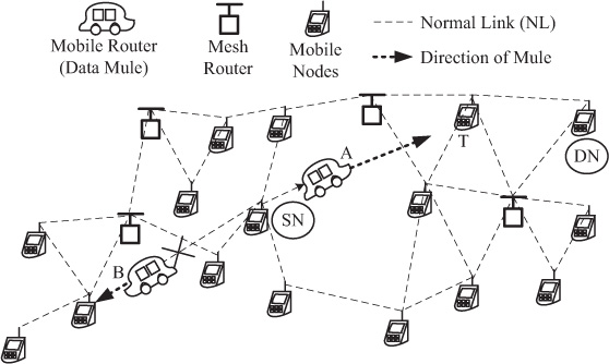
Figure 6.12. Data loading in data-mule-based non-persistent new link addition

Data packets can be forwarded to the mule either in the active mode or in the passive mode. In active forwarding, the DN is known in advance; therefore, the motion of the data mule can be controlled. On the contrary, passive forwarding deals with unknown DN. In passive forwarding mode, opportunistic transmission takes place. Opportunistic transmission is further subdivided into three categories: (i) no forwarding, (ii) all forwarding, and (iii) selective flooding. For no forwarding, the data mule just receives the data packet from the SN and buffers the data until it gets clearance from the DN. In the case of all forwarding, the mobile node exchanges the data packets with all the nodes to its contact. Therefore, data delivery rate is maximized for all forwarding scenarios with the expense of massive data packet flooding in the network. Selective flooding, on the other hand, is based on the greedy routing mechanism and geographical routing. The data mule forwards the data packets to the node nearer to the DN when selective flooding is concerned. The length of LL, based on the data mule approach, is the distance covered by the mules from the SN to the DN.

The strategy of using a data mule is not possible when a stationary SWWMN is concerned. However, the router nodes in WMNs are situated in fixed locations in the network. Therefore, mobile mesh routers are required to implement the data-mule-based LL addition strategy, which is challenging in WMNs.

Advantages and Disadvantages of Data-Mule-Based SWWMNs

The advantages of data-mule-based LL creation are the following. (i) Data-mule-based strategy can be applied in the context of delay-tolerant networking where data packets need to be transported to the distant storage device or another router node that is situated far away. (ii) No physical deployment of LLs is needed to transport data in the network.

However, the major disadvantage of implementing data mule in SWWMNs is its complexity in establishing a data-mule-based LL by identifying the actual direction of a DN.

6.10.2 Load-Aware Long-Ranged Link Creation

Load-aware non-persistent LL (NPLL) deploys a set of smart routers (SRs) to create LLs in a WMN, which may change their positions after a certain time period [126]. An SR is a wireless mesh router equipped with a smart antenna which is capable of forming a highly directional beam and then changing direction of the beam adaptively to make NPLLs in an SWWMN. NPLLs, for a specific time duration, can be created among SRs to exchange data packets among a set of SNs and DNs. For the creation of an NPLL, an SR node pair has to satisfy a cut-off distance, as shown in Figure 6.13. Note that cut-off distance between an SR node pair represents the EHD between two SR nodes in the network.

Figure 6.13 explains the NPLL creation strategy in an SWWMN where the cut-off distance of an NPLL is set to be 2 ≤ EHD ≤ 6. In the figure, SR₁ can create NPLLs either with SR₂ (NPLL₁ in Figure 6.13) or with SR₃ (NPLL₂) for a stipulated time interval, as the EHDs among SR₁–SR₂ and SR₁–SR₃ are three and four hops which satisfy the cut-off value for the network. However, NPLL₃ between SR₁ and SR₄ cannot be created as the EHD between the two nodes is 7, which does not reside within the range of the cut-off value to create an NPLL.

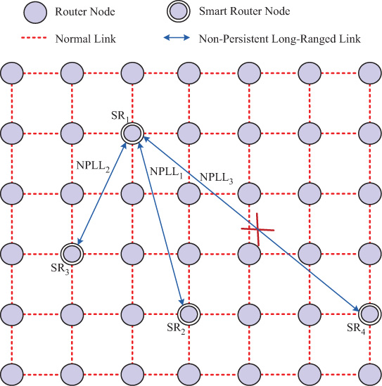
An illustration of Non-Persistent link creation by smart routers in an SWWMN.

Figure 6.13. Non-persistent link creation by smart routers in an SWWMN

NPLLs, which can only be established among SR node pairs, are used for data transmission among distant SNs and DNs. Since NPLLs are typically expensive, edge weights can be assigned in order to use the NPLLs in a limited manner. However, an NPLL can be used for data transmission until it reaches the maximum bearable load, after which it is disabled for further data transmission in the SWWMNs. Thereafter, data transmission has to be carried out through existing NLs and other NPLLs. Load balancing, which is implemented to better distribute the traffic load throughout the NPLLs, is depicted in Figure 6.14.

In Figure 6.14, it is assumed that the maximum load that an NPLL can handle is equal to 2 units. Now, NPLL₁ between SR₁ and SR₂ is used to carry out a data transmission session between SN₁ and DN₁. Hence, the NPLL is used first to make a shortest path in the SWWMN. Now, to have a data transmission between SN₂ and DN₂, NPLL₁ is deployed a second time as NPLL₁ resides in the shortest path between SN₂ and DN₂. For the data transmission from SN₃ to DN₃, the shortest path can again be created through NPLL₁. However, as the maximum load of an NPLL in the network is set to be 2, NPLL₁ already reaches its maximum limit of data transfer. Therefore, the NPLL cannot be used in the data transmission from SN₃ to DN₃ as can be seen in Figure 6.14.

An illustration of Load balancing strategy for non-persistent LLs in SWWMN.

The components along with their symbols used in the network are listed above as follows: a single circle for a Router Node, two concentric circles for a Smart Router Node, a red dashed line for a Normal link, a blue bi-directional arrowhead for Non-Persistent Long-Ranged Link, a dashed black arrow for Completed Data Session, and a dashed grey arrow for Uncompleted Session. A 6 cross 7 grid, with a Router Node, placed over the vertices of the grid is present. Each router is connected to every other router around it by dotted lines. The Router Nodes at the following positions are labeled thus: (1, 3) as SN1, (5, 5) as SN2, (3, 3) as SN3, (4, 4) as DN1, (2, 4) as DN2, and (6, 3) as DN3. The Router Nodes in the following positions are replaced by Smart Router Nodes labeled thus: (2, 3) as SR1, (5, 4) as SR2, (4, 2) as SR3, and (4, 7) as SR4. A Non-Persistent Long-Ranged Link represented by a blue bi-directional arrow runs between SR1 and SR2 and is labeled NPLL1. The following black dashed arrows representing Completed Data Sessions point from and to the following nodes: SN1 to SR1, SR1 to DN2, SR1 to SR2 labeled SN1 DN1, SN2 to SR2, SR2 to DN1, and SR2 to SR1 labeled SN2 DN2. An Uncompleted Data Session denoted by a dashed grey arrow runs from and to the following nodes: SR1 to SR2 labeled SN3 DN3, SR2 and the node at position (6, 4), this node and DN3, SN3 to SR1. An X-mark is placed over the link SN3 DN3. On the top of the grid, the Maximum load per non-persistent LL is said to supposedly equal 2.

Figure 6.14. Load balancing strategy for non-persistent LLs in SWWMN

Furthermore, during the creation of NPLLs, if multiple NPLLs are partially overlapped or assigned in the same orientation, it may result in interference. In such scenarios, the interfering NPLLs share the alloted NPLL bandwidth. For example, if two NPLLs are superimposed in an SWWMN, then the allotted spectrum for each of the overlapped NPLLs becomes halved.

Advantages and Disadvantages of NPLLs

The advantages of load-aware LL creation are the following. (i) Based on the requirement, NPLLs can change their directions so that efficient data transmission can take place. (ii) Load balancing in NPLLs results in overall traffic fairness in SWWMNs.

However, the main disadvantages in the context of NPLL creation are (i) interference between NPLLs and NLs, and (ii) beam steering of smart antennas in real-time applications.

6.11 Non-Persistent Routing in Small-World Wireless Mesh Networks

A load-aware non-persistent small-world LL routing (LNPR) algorithm, which finds the shortest path greedily to transfer data from an SN to a DN in an SWWMN without causing significant overloading of NPLLs, is described in this section. LNPR also incorporates load balancing, which results in better traffic distribution among NLs as well as NPLLs in the SWWMNs [126].

A small number of bidirectional NPLLs are deployed, before applying the LNPR algorithm, in an SWWMN. In order to use the NPLLs in a limited manner, each NPLL can be allotted an edge weight which can be determined as described in Algorithm 6.5. An NPLL is created if it satisfies the lower and upper limits of the EHDs between an SR node pair in an SWWMN (lines 4–6). Note that there cannot be unlimited NPLLs, as their number is bounded by NPLL_max, which is the maximum possible NPLLs, for an SWWMN. Now, the edge weight assignment for a certain NPLL is evaluated as follows:

Calculate APL for a network without adding i^th NPLL.
Add i^th NPLL and again calculate APL of the network.
Calculate $N P L L_{E d g e W e i g h t} (i) = (\frac{A P L}{A P L (i)}) \times S F$ $N P L L_{E d g e W e i g h t} (i) = (\frac{A P L}{A P L (i)}) \times S F$ and assign to i^th NPLL, where APL(i) is the APL with i^th NPLL and SF is the scaling factor which is greater than or equal to 1 unit (lines 7–8).

In Algorithm 6.5, NPLLs are deployed among SR node pairs based on the path differences through NLs in the network. The path traversed between an SN and a DN is denoted as the end-to-end hop distance through NLs (EHD_NL(SN, DN)) in an SWWMN. To determine the edge weight of an NPLL, the ratio of the APL of an SWWMN is calculated with only NLs to the APL of the network including the newly added NPLL. Hence, the edge weight of an NPLL in an SWWMN is the ratio of APLs of the network with and without the deployment of an NPLL, as depicted in line 7 in Algorithm 6.5. Therefore, an NPLL that results in a lower APL for the WMN is assigned higher edge weight in the network.

By calculating the metric NPLL_EdgeWeight, higher edge weight to the more important NPLLs is assigned in the SWWMN. Thus, the NPLLs can be used efficiently to create a path between the SN and DN in the SWWMN without severe overloading. However, the edge weight for each NPLL is very small. Therefore, a metric, scaling factor (SF) can be considered to enhance the edge weight uniformly for each NPLL in the network.

Algorithm 6.5 Determination of Edge Weight for NPLL

Require:

$𝒢 = (𝒩, ℰ)$ $? = (?, ℰ)$ — Graphical representation of a wireless mesh network with $𝒩$ $?$ nodes and $ℰ$ $ℰ$ links

SN — Source node in $𝒢$ $?$

DN — Destination node in $𝒢$ $?$

SR — Smart router node in $𝒢$ $?$

NL — Normal link in $𝒢$ $?$

NPLL — Non-persistent bidirectional long-ranged link (LL) in $𝒢$ $?$

NPLL_max — Maximum number of possible NPLLs in $𝒢$ $?$

EHD — End-to-end hop distance between SN and DN (including NLs and NPLLs)

EHD_NL(SN, DN) — EHD between SN and DN only through NLs

SR_total — Total number of SR nodes in $𝒢$ $?$

LowerLimit_NPLL — Lower boundary of EHD_NL(SN, DN)

U pperLimit_NPLL — Upper boundary of EHD_NL(SN, DN)

SF — Scaling factor ≥ 1

APL — Average path length of G without NPLL

APL(i) — APL of G with i^th NPLL

NPLL_EdgeWeight(i) — Edge weight of i^th NPLL in $𝒢$ $?$

Initialization: NPLL_max, LowerLimit_NPLL, and U pperLimit_NPLL

1: k ← 0

2: for i = 1 → (SR_total − 1) do

3: for j = i + 1 → SR_total do

4: if LowerLimit_NPLL ≤ EHD_NL(i, j) ≤ U pperLimit_NPLL then

5: k ← k + 1

6: Create k^th NPLL between i^th and j^th SR node pair

7: $N P L L_{E d g e W e i g h t} (k) = (\frac{A P L}{A P L (k)}) \times S F$ $N P L L_{E d g e W e i g h t} (k) = (\frac{A P L}{A P L (k)}) \times S F$

8: Assign NPLL_EdgeWeight(k) to k^th LL

9: if k > NPLL_max then

10: go to 14

11: end if

12: end if

13: end for

14: end for

6.11.1 Load-Aware Non-Persistent Small-World Routing

To evaluate end-to-end path distance among a few randomly chosen SN-DN pairs with LNPR, in Algorithm 6.6, shortest paths are measured with a greedy approach (line 6). To incorporate the strategy of load balancing, the following steps are deployed in the LNPR algorithm (lines 7–15) to evenly distribute the load in the network.

Algorithm 6.6 Load-Aware Non-Persistent Small-World Routing (LNPR)

Require:

$𝒢 = (𝒩, ℰ)$ $? = (?, ℰ)$ — Graphical representation of a wireless mesh network with $𝒩$ $?$ nodes and $ℰ$ $ℰ$ links

SN — Source node in $𝒢$ $?$

DN — Destination node in $𝒢$ $?$

SR — Smart-router node in $𝒢$ $?$

NL — Normal-link in $𝒢$ $?$

NPLL — Non-persistent bidirectional long-ranged link (LL) in $𝒢$ $?$

NPLL_EdgeWeight(i) — Edge weight of i^th NPLL in $𝒢$ $?$

ConnectionLink(i) — i^th link (NL or NPLL) between a node pair in $𝒢$ $?$

RecursiveCall_max — Maximum number of possible recursive calls to find a shortest path in $𝒢$ $?$

MaxLoad_NL — Maximum traffic load that an NL can handle

MaxLoad_NPLL — Maximum traffic load that an NPLL can handle

Initialization: RecursiveCall_max, MaxLoad_NL, and MaxLoad_NPLL

1: Assign NPLL_EdgeWeight to all NPLLs in $𝒢$ $?$ (see Algorithm 6.5)

2: Random_SN−DN ← Number of randomly chosen SN-DN pairs in $𝒢$ $?$

3: for i = 1 → Random_SN−DN do

4: Count ← 0 // To track RecursiveCall_max

5: while Count ≤ RecursiveCall_max do

6: Path_Shortest ← Shortest path between SN_i and DN_i in $𝒢$ $?$

7: for j = 1 → (Path_Shortest − 1) do // Implementation of load-balancing

8: if ConnectionLink(j) ← (MaxLoad_NL || MaxLoad_NPLL) then

9: Disable j^th link for rest of the data transfer session

10: Count ← Count + 1

11: if Count > RecursiveCall_max then

12: go to 16 // No more shortest path possibilities exist

13: end if

14: end if

15: end for

16: end while

17: if Path found in $𝒢$ $?$ between SN_i and DN_i then

18: Transfer data packets between SN_i and DN_i through Path_Shortest

19: end if

20: end for

Check for each connection link (both NLs and NPLLs) in a shortest path between an SN-DN pair to identify whether it reaches its maximum possible load.
If the link reaches its maximum load, disable the link for the rest of the data transmission sessions.
Search for another shortest path between the SN-DN pair if the shortest path searching does not reach the maximum value (RecursiveCall_max in Algorithm 6.6).

If a shortest path between an SN-DN pair is found after implementing load balancing with LNPR, a data transfer session is carried out in the network (lines 17–19). The performance of the LNPR-based approach is discussed in the following.

6.11.2 Performance Evaluation of LNPR Algorithm

The performance of the LNPR algorithm is experimented in a grid network of 100 mesh router nodes positioned in a 10 × 10 square-grid topology [126]. SR nodes are deployed randomly in the network (5% of the total number of nodes in the WMN) to create NPLLs. SN and DN pairs are randomly chosen from the grid WMN. Performance of the LNPR algorithm is briefly discussed here.

Observations on Call Blocking Probability

Call blocking probability (CBP) is a metric which determines the probability of blocked call averaged over a data transmission session in the network. If NLs exceed weighted MaxLoad_NL or NPLLs exceed weighted MaxLoad_NPLL after a few attempts, it can be concluded that the call is dropped in the SWWMN (Algorithm 6.6). Hence, CBP is calculated as the ratio of total blocked calls to the total number of calls for data transfer sessions in the SWWMNs. Figure 6.15 shows that reduction in CBP with LNPR as compared to CBP without LNPR for different sets of SN-DN pair ranging from 58% (50 SN-DN pairs) to 95% (30 SN-DN pairs) with SF is equal to 3. Here, SF denotes the edge weight that is assigned to a link based on its impact in the SWWMN.

A vertical bar graph showing the relationship between Number of SN-DN Pairs and the Call Blocking Probability with and without LNPR.

The horizontal axis is marked with the Number of SN-DN Pairs from 0 to 50 in the increments of 10. The vertical axis is marked with the Call Blocking Probability (CBP) from 0 to 0.14 in the increments of 0.02. A legend on the top shows that the blue and red bars denote CBP without and with LNPR, respectively. At 20 along the horizontal axis, the blue bar ranges to 0.035 and its I-bar ranges from 0.01 to 0.06; while the red bar reaches 0.005 and its I-bar ranges from 0 to 0.02. When there are 30 pairs of SN-DN, the blue bar reaches 0.08 with an I-bar ranging from 0.039 to 0.121; while the red bar reaches 0.004 with its I-bar ranging from 0 to 0.057. At 40 along the horizontal axis, the blue bar ranges to 0.073 and its I-bar ranges from 0.039 to 0.105; while the red bar reaches 0.019 and its I-bar ranges from 0.005 to 0.03. When there are 50 pairs of SN-DN, the blue bar reaches 0.079 with an I-bar ranging from 0.033 to 0.107; while the red bar ranges up to 0.036 with its I-bar ranging from 0.1 to 0.57. All values are approximate.

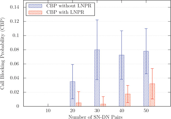
Figure 6.15. Call block probability with and without LNPR (SF = 3)

Observations on Load Balancing

Figure 6.16 depicts the variation of the maximum load with and without LNPR with SF = 3, as it is the optimum value of SF under the conditions used for simulations. Furthermore, maximum load is the same for NPLLs with and without LNPR, whereas when the SN-DN pairs increase from 20 to 50, decrement of the maximum load with LNPR for different sets of SN-DN pair ranges from 23% (20 SN-DN pairs) to 70% (50 SN-DN pairs) as compared to maximum load without LNPR in the SWWMN. With SF = 3, it can be seen that the maximum load for LNPR is much lower than without LNPR.

Observations on Average Transmission Path Length

Average transmission path length (ATPL) is the EHD between SN and DN averaged over a set of data transmission sessions for a stipulated time in the WMN. ATPL gives a measure of reduced path length with the help of NPLLs in the SWWMN. ATPL gives the measure of transmission path length for a set of data sessions, whereas APL is defined as average path length of the whole network. Figure 6.17 shows the ATPL observations for various cases.

Figure 6.17 shows the ATPL values with NLs (normal ATPL), small-world ATPL without LNPR (SW-ATPL without LNPR), and small-world ATPL with LNPR algorithm (SW-ATPL with LNPR) for 10 SN-DN pairs to 50 SN-DN pairs of data transmission. From the figure, it is clear that after implementing NPLLs in the network, ATPL is decreased significantly compared to normal ATPL. From Figure 6.17, to determine ATPL with NPLLs with different sets of SN-DN pairs, reduction achieved in ATPL is from 15% (30 SN-DN pairs) to 20% (10 SN-DN pairs) with respect to ATPL with only NLs in the network. However, it can be observed that the value of ATPL is slightly increased when LNPR is used. From Figure 6.17, it can be seen that the set of SN-DN pairs increase from 10 to 50, only a small increment from 0.7% (20 SN-DN pairs) to 9% (50 SN-DN pairs) is observed in the ATPL value for LNPR algorithm compared to SWWMN with NPLLs.

A vertical bar graph showing the relationship between Number of SN-DN Pairs and the Maximum Load of NPLLs with and without LNPR.

The horizontal axis is marked with the Number of SN-DN Pairs from 0 to 50 in the increments of 10. The vertical axis is marked with the Maximum Load of NPLLs from 0 to 12 in the increments of 2. A legend on the top shows that the blue and red bars denote the Maximum Load without and with LNPR, respectively. At 10 along the horizontal axis, both the blue and red bars range to 2.2 and their I-bars range from 1.6 to 3.1. When there are 20 pairs of SN-DN, the blue bar reaches 3.9 with an I-bar ranging from 3.4 to 4.9; while the red bar reaches 3. At 30 along the horizontal axis, the blue bar ranges to 5.8 and its I-bar ranges from 4.2 to 5.2; while the red bar reaches 3. When there are 40 pairs of SN-DN, the blue bar reaches 9 with an I-bar ranging from 7.2 to 11; while the red bar ranges up to 3. At 50 along the horizontal axis, the blue bar ranges to 10.8 and its I-bar ranges from 8.2 to 12.2; while the red bar reaches 3. The red bars from 20 to 50 do not have I-bars. All values are approximate.

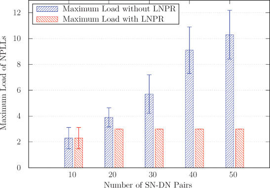
Figure 6.16. Maximum load of NPLLs with and without LNPR (SF = 3)

A vertical bar graph showing the relationship between Number of SN-DN Pairs and the Average Transmission Path Length with NLs, and with and without LNPR.

The horizontal axis is marked with the Number of SN-DN Pairs from 0 to 50 in the increments of 10. The vertical axis is marked with Average Transmission Path Length (ATPL) values from 0 to 10 in the increments of 2. A legend on the top shows that the blue, red, and green bars denote the ATPL with NLs, SW-ATPL without LNPR, and SW-ATPL with LNPR, respectively. At 10 along the horizontal axis, both the blue bar ranges up to 6.3 with its I-bar from 5.8 to 7; the red and green bars range up to 5 and their I-bars range from 4.3 to 5.6. When there are 20 pairs of SN-DN, the blue bar reaches 6.9 with an I-bar ranging from 6.4 to 7.4; the red bar reaches 5.6 with I-bar from 5.4 to 5.8; and the green bar reaches 5.7 with its I-bar ranging from 5.5 to 5.9. At 30 along the horizontal axis, the blue bar ranges to 6.8 and its I-bar ranges from 6 to 7.7; the red bar reaches 5.7 with its I-bar ranging from 5.6 to 6.1; and the green bar ranges up to 5.9 with its I-bar from 5.6 to 6.8. When there are 40 pairs of SN-DN, the blue bar reaches 6.7 with an I-bar ranging from 6 to 7; while the red bar ranges up to 5.6 and has an I-bar that reaches from 5 to 5.9; and the green bar ranges up to 5.8 with an I-bar from 5.8 to 6.2. At 50 along the horizontal axis, the blue bar ranges to 6.9 and its I-bar ranges from 6.5 to 7; while the red bar reaches 5.7 with an I-bar ranging from 5.5 to 5.8; and the green bar reached 6.1 and had an I-bar ranging from 5.8 to 6.4. All the values are approximate.

Figure 6.17. ATPL with NLs, SW-ATPL without LNPR, and SW-ATPL with LNPR

Therefore, the application of LNPR algorithm results in substantial distribution of the traffic load, which reflects in the maximum load distribution among the NPLLs and the minimization of the network call block probability.

Advantages and Disadvantages of LNPR-Based SWWMNs

The advantages of LNPR-based LL creation are the following. (i) The LNPR-based approach takes into account the maximum load carrying capability for each existing link in an SWWMN. (ii) LNPR also improves the call blocking probability for the network.

However, the main challenge of implementing the LNPR-based approach is (i) the deployment of NPLLs, which requires a precision beam steerer for directional antenna to create an NPLL in the network.

6.12 Qualitative Comparison of Existing Solutions

The existing approaches on the creation of SWWMNs are summarized in Table 6.2. Moreover, the basis of LL creation along with the reason of implementation of the small-world concept are provided in Table 6.2.

Table 6.2. Qualitative comparison of existing models on small-world networks

Nature of LLs	Creation Strategy	Basis of Small-World Creation	Main Objective	Applicability to WMNs
Persistent LL	Random Creation	Random Rewiring [6]	Reduction in APL	Most Complex
		Pure Random Addition [68]	Calculate the scaling forms and single critical exponent of critical region of the network	Moderate
		Euclidean Distance [69]	Shortest path between SN and DN	Moderate
		Based on [2,r] Hops [94]	Contact-based distributive algorithm	Moderate
		Genetic Algorithm [123]	To find minimum number of LL required	Moderate
		Uneven Probabilistic Flooding [119]	Shorter path	Easy
		Power Control and Beamforming [120]	Enhancement of end-to-end throughput	Easy
		Single-Gateway Router Based [95]	To lower G-APL	Moderate
		Multi-Gateway Router Based [122]	To achieve load balancing	Moderate
		Randomized Beamforming [121]	Distributive algorithm design	Moderate
		Cooperative Communication Based [124]	Shorter path length	Complex
	Deterministic Creation	Based on MinAPL [72]	Minimize average path length	Moderate
		Based on MinAEL [72]	Minimize average edge length	Easy
		Based on MaxBC [72]	Maximize network betweenness centrality	Moderate
		Based on MaxCC [72]	Maximize network closeness centrality	Moderate
		Based on MaxCCD [72]	Minimize average network delay	Easy
		Sequential Deterministic LL Addition (SDLA) [77]	Shortest path	Easy
Non-persistent LL	Random Creation	Data Mule Based [125]	Shorter path	Complex
	Random Creation	Load-Aware Link Addition [126]	Shorter path	Complex
	Routing Algorithm	LNPR [126]	Shorter path	Complex

It can be observed from Table 6.2 that most of the existing LL creation strategies (i.e., rewiring or addition of LLs) are based on the deployment of persistent LLs. As the mesh clients in a WMN are mobile in nature, it is very challenging to implement data-mule-based non-persistent LLs. Moreover, the data-mule-based strategy requires additional information regarding the location of the DN and the position of the mobile data mules in the wireless network [125]. On the other hand, non-persistent LLs can also be created based on the beam steering technique. One of the non-persistent LL creation discussed in this chapter based on the LNPR strategy, which also takes care of load balancing in the SWWMNs [126]. Furthermore, it can also be observed that the CBP is improved when LNPR-based LL addition is concerned. However, implementing the strategy in an SWWMN is still a challenging task.

The rewiring of existing NLs is also difficult to realize in the context of WMNs. To implement the rewiring concept in a WMN, the direction of the antenna beam in the existing network has to steer in order to connect to another distant node. Therefore, the antenna element has to perform two consecutive operations to successfully rewire an NL to an LL in a WMN. First, the direction of the antenna beam has to change in the existing network, and then the power of the transmission has to increase to make connection with some distant node. This operation requires prior information about the network, and some adaptive control also has to be applied to rotate the antenna in certain specified direction. Therefore, rewiring of existing NLs in a WMN is complex to realize [6], [94].

Most of the existing small-world creation models attempt to reduce the APL value by creating shortcuts in order to minimize the EHDs between node pairs in a network. In pure random link addition strategy, small-world characteristics bring down the finite-sized scaling metric and the critical exponent for the critical region of the network [68]. End-to-end throughput can also be enhanced by means of improving the transmission power and deploying directional beam-former to enhance the per-hop throughput in the SWWMNs [121], [119], [120]. On the other hand, GA-based LL addition strategy minimizes the number of added LLs based on the genetic algorithm approach [123]. Cooperative router nodes can also be deployed to minimize the EHDs of the SWWMNs [124]. Furthermore, C-SWAWN-based protocol can also be beneficial while designing efficient SWWMNs in the context of single and multi-gateway router scenarios [122], [95]. The LL deployment with LM-GAS strategy addresses the critical issue of load balancing in the context of WMNs.

Small-world characteristics can also be incorporated by adding new LLs with deterministic decisions [72], [77]. LLs can be added deterministically based on various strategies such as MinAPL, MinAEL, MaxBC, and MaxCC. All of these strategies are exhaustive search–based approaches and thus take a long time to determine the LL connecting locations in the network. However, heuristic approaches such as MaxCCD and SDLA can also be used where time complexity of LL addition reduces without affecting overall network performance. Table 6.2 provides a comparative study of the existing small-world creation approaches and their applicability in the context of SWWMNs.

6.13 Open Research Issues

There exist many open research issues in the context of SWWMNs. In the following, a set of such open research issues are discussed.

Lower End-to-End Delay: In the case of WMNs, end-to-end delay in transmission is a very critical parameter as WMNs support multi-hop relaying of data packets from SN to DN. By implementing a small number of LLs in the existing WMN, the EHD can be minimized. Therefore, end-to-end delay in transmission remains a critical design objective for WMNs. Moreover, network throughput of a WMN is affected by the delayed transmission of the data packets from a source to its destination. Therefore, the rate of data packet transmission is decreased with increasing end-to-end delay in the wireless network. Hence, optimization of the end-to-end delay in the SWWMN is an open research issue. Further, the design of SWWMNs for minimizing end-to-end delay in the presence of heterogeneous physical transmission link is another open problem.
In-band Operation for NL and LL: In a SWWMN, LLs are created by the highly directional antennas operating in different frequency bands with respect to the NLs in WMNs. Therefore, LLs use out-of-band frequency to create a SWWMN. However, this out-of-band operation to implement small-world characteristics in a WMN results in inefficient utilization of bandwidth, which is a scarce resource. Moreover, availability of additional bandwidth to implement LLs is difficult. Therefore, out-of-band operation of the SWWMN is not fulfilling the ultimate goal of capacity enhancement of the network.

One solution is to incorporate LLs and NLs in the same frequency band. However, the simultaneous in-band operation of NLs and LLs may introduce severe interference in the transmission of data packets, which will affect signal to interference and noise ratio (SINR). Hence, the network capacity of a WMN will be affected as SINR is directly proportional to the network throughput. Therefore, some trade-off is required to fulfill the desired goal of maximization of the throughput in SWWMN. Therefore, design of in-band LL-based SWWMN remains an open research area.
Routing Protocol for SWWMNs: Routing of data packets among the mesh nodes is another critical design issue of SWWMNs. The existing routing protocols are only concerned about the routing through NLs. However, the cooperative routing concept to implement SWWMN can be one of the solutions where the cooperative links can be used for routing [124]. Furthermore, load-aware non-persistent LL creation via smart router nodes can be considered as another possible solution [126]. Presently, the routing protocols of MANETs with some modifications are typically used in the WMNs. However, many of those protocols do not give optimized performance in the context of SWWMNs. Therefore, design of optimized routing algorithm for SWWMNs is another open research issue.
Cognitive Radio–based SWWMNs: Cognitive radio (CR) is an open research area in the context of SWWMNs. A WMN operates in the ISM (Industrial, Scientific and Medical) band, which is very crowded. Therefore, it is difficult to allocate more bandwidth in the ISM band for the creation of LLs to get a SWWMN. CR is one of the choices which can be incorporated to make use of the licensed unused band whenever possible without impairing any operational difficulties for the licensed users.

The main aim of CR is to find the white space (unused space) in the licensed frequency band, and borrow that band for the unlicensed users. Therefore, CR-based SWWMN may use the borrowed frequency band to create LLs in the network.
Adaptive Beam Steering in LNPR: LNPR is a load-balanced routing protocol that can be deployed in the SWWMNs. However, in LNPR, beam steering of the SRs to other reachable SRs are mostly based on the traffic demand and a scheduling strategy. However, no such technique yet exists for steering the beam toward certain SR nodes based on the practical requirement. Therefore, development of an adaptive beam steering technique in the context of LNPR strategy is another open research issue.
Load Balancing in SWWMNs: In SWWMNs, LLs act as transmission highways. Therefore, a huge amount of traffic has to be carried out by most of the LLs. Moreover, due to their multi-hop relaying nature, mesh router nodes which are situated near the central region of the network face severe traffic. Hence, to avoid the traffic imbalance in LLs as well as central router nodes, optimal load-balancing strategies need to be developed for the SWWMNs. Development of optimal load-balancing strategies is an open research problem.

6.14 Summary

This chapter discussed SWWMNs to improve the performance of traditional WMNs. A typical WMN consists of mesh clients, mesh routers, and gateway mesh routers. Mesh clients can be any mobile devices which are connected to the mesh routers, which are mostly fixed in a WMN, and the mesh routers are connected to the Internet or any infrastructure networks through the gateway routers in a multi-hop fashion. Adding a few LLs among static mesh routers can drastically improve overall network operation by minimizing the end-to-end hop distances in the network. In this chapter, various LL creation strategies in an SWWMN are classified into two major categories: persistent LL creation and non-persistent LL creation. The persistent LL creation strategy, which does not change location of an LL with time, is further divided into random creation of a few LLs to create SWWMNs and small-world network creation by deterministic approaches. It can also be observed that the method of new LL addition is practically deployable in the context of WMNs compared to rewiring. In the non-persistent LL creation strategy, where an LL may change its location with time, prior information regarding the position of the network nodes is required to deploy LLs in the network. The main objectives of the existing approaches to implement LLs and their applicability in the context of WMNs were thoroughly discussed. The chapter also presented a qualitative comparison of the existing strategies and their implementation complexities when SWWMNs were concerned. Finally, some of the open research issues in SWWMNs were also highlighted.

Exercises

1. Survey the literature on wireless mesh networks and identify the reasons that can degrade the performance of wireless mesh networks.

2. Write a program to simulate a wireless mesh network with N nodes and M links where M > N. Each node is associated with an (x, y) coordinate on a 2-D plane. Add k LLs randomly and estimate the reduction in APL, ACC, and AND. Consider a slightly different method of link addition where k links are added between a randomly selected node and a central node in the network. The central node can be chosen as the node with the highest closeness centrality in the network. What are your observations on the APL values for these two cases?

3. Rewiring is a small-world network creation strategy where one end of an already existing link of a network is removed and connected to another distant node in the network. However, rewiring strategy imposes some challenges in the context of wireless multi-hop relaying networks. Identify and list the challenges faced in link rewiring in a WMN which is a type of multi-hop relying networks.

4. Consider a ring topology network with 20 nodes. Each node in the network has neighbor degree 4. Apply the Watts-Strogatz rewiring strategy with rewiring probability p ∈ {0.02, 0.05, 0.1, 0.5, 1}. Calculate APL, ACC, and AND for each case. What are your observations on the resultant network structures with different p values?

5. Write a program to simulate Kleinberg’s 2-D grid model (with sufficiently large size, e.g., 10,000 nodes) where you need to add five LLs based on Euclidean distance between the nodes. The experiment should be performed for the following cases: (i) α = 1, (ii) α = 2, and (iii) α = 3, where α is the clustering coefficient. Comment on the observations.

6. The existing Euclidean distance–based LL addition strategy (i.e., Kleinberg’s model) does not consider mobile nodes while creating an LL. Develop a Euclidean distance–based LL addition algorithm to accommodate mobile mesh nodes for an SWWMN.

7. Consider an unweighted and undirected wireless network, as shown in Figure 6.18. Identify the nodes with the highest wireless flow betweenness. What are the impacts on the resources of the nodes with high WFB?

An unweighted and undirected wireless network with six nodes is displayed.

Figure 6.18. An example network for Problem 7

8. Write a computer program to create a small-world network topology with one gateway router. Add k LLs, where k ≥ 5, by varying the Δ parameter. Find out the impact of different values of Δ in the G-APL obtained. Plot a graph for the G-APL and Δ.

9. How could you modify the GAGS algorithm such that the optimal value of Δ_h can be achieved?

10. Consider a string topology wireless mesh network which is deployed along a highway. However, due to the sparseness, end-to-end hop distance of the mesh network is high. As a result, delay incurred in the network is too high, which in turn degrades overall network performance. However, a few LLs can improve the scenario. Simulate such a situation by taking 20 mesh router nodes deployed as a string topology network. Add three deterministic LLs, which can optimize network APL (i.e., MinAPL-based LL addition strategy). Comment on the time consumed by your program to add the LLs. Now, add the same number of LLs with the SDLA algorithm and the compare the APL with the MinAPL. Also comment on the time consumed to execute SDLA.

11. Identify some real-world situations in social networks, biological networks, or technological networks where data mules can be observed.

12. Can the LNPR algorithm be used for all types of networks? Consider a network with certain edges that act as bridge nodes where removal of those edges can result in network partitioning. Suggest a mechanism to improve LNPR to work in networks with bridge links.

13. Estimate the time complexity for the following algorithms: data-mule-based LL addition, SWCR-based LL addition, and SWCR-based LL addition algorithms.

14. What are the implications of load balancing with LNPR? Develop a computer program to add k LLs (where k ≥ 1) in a 10 × 10 grid network. Note that the LL addition should not consider load balancing. Make observations on the performance of the algorithm when CBP and ATPL values are concerned. Compare the results when load balancing is incorporated. Make suitable assumptions.

15. Modify the LNPR algorithm such that it can be implemented when a set of bridge links is present in the network. Here, a bridge link means that one end of the link must be connected to a pendant node.

16. Consider a five-node string topology WMN, as shown in Figure 6.19. Note that each node is a mesh router, and there is no possibility that, apart from the path as can be seen in the figure, an alternative route exists in the network. Now estimate the network throughput for the following scenarios: the bidirectional link between two mesh routers is unweighted, the range of wireless transmission of each of the mesh router is approximately 100 meters, and the data transmission rate can be assumed to be 0.1Mbps.

Figure 6.19. An example network for Problem 16

1. In the physical world, phase transition happens when an object changes its state from solid to liquid, then to gaseous state, and so on. In a network with rewiring, similarly, a regular network gradually transforms to a small-world network and then to an arbitrary random network with increasing rewiring probability p.

..................Content has been hidden....................

You can't read the all page of ebook, please click here login for view all page.

Table of Contents for 6 Small-World Wireless Mesh Networks

Create new playlist

Sign In

Sign Up

Chapter 6Small-World Wireless Mesh Networks

6.1 Introduction

6.1.1 The Small-World Characteristics

6.1.2 Small-World Wireless Mesh Networks

6.2 Classification of Small-World Wireless Mesh Networks

6.3 Creation of Random Long-Ranged Links

6.3.1 Random LL Creation by Rewiring the Normal Links

Advantages and Disadvantages of Rewiring-Based SWWMNs

6.3.2 Random LL Creation by Addition of New Links

6.4 Small-World Based on Pure Random Link Addition

Advantage and Disadvantage of Pure Random Link Addition–Based SWWMNs

6.5 Small-World Based on Euclidean Distance

Advantages and Disadvantages of Euclidean Distance–Based SWWMNs

6.6 Realization of Small-World Networks Based on Antenna Metrics

6.6.1 LL Addition Based on Transmission Power

Advantages and Disadvantages of Transmission Power–Based SWWMNs

6.6.2 LL Addition Based on Randomized Beamforming

Advantages and Disadvantages of Randomized Beamforming-Based SWWMNs

6.6.3 LL Addition Based on Transmission Power and Beamforming

Advantage and Disadvantage of Transmission Power and Beamforming–Based SWWMNs

6.7 Algorithmic Approaches to Create Small-World Wireless Mesh Networks

6.7.1 Contact-Based LL Creation

Advantage and Disadvantage of Contact-Based SWWMNs

6.7.2 Genetic Algorithm–Based LL Addition

Advantage and Disadvantage of GA-Based SWWMNs

6.7.3 Small-World Cooperative Routing–Based LL Addition

Advantage and Disadvantage of SWCR-Based SWWMNs

6.8 Gateway-Router-Centric Small-World Network Formation

6.8.1 Single Gateway-Router-Based LL Addition

Random LL Addition Strategy-Based SWWMNs

Time Complexity of RAS

Gateway-Aware LL Addition Strategy–Based SWWMNs

Time Complexity of GAS

Gateway-Aware Greedy LL Addition Strategy–Based SWWMNs

Time Complexity of GAGS

Advantages and Disadvantages of Single Gateway-Router-Based SWWMNs

6.8.2 Multi-Gateway-Router-Based LL Addition

Multi-Gateway Aware LL Addition Strategy–Based SWWMNs

Load-Balanced Multi-Gateway-Aware LL Addition Strategy–Based SWWMNs

Time Complexity of LM-GAS

Advantages and Disadvantages of Multi-Gateway-Router-Based SWWMNs

Comparison of Gateway-Router-Based LL Addition Strategies

6.9 Creation of Deterministic Small-World Wireless Mesh Networks

6.9.1 Exhaustive Search–Based Deterministic LL Addition

6.9.2 Heuristic Approach-Based Deterministic LL Addition

6.10 Creation of Non-Persistent Small-World Wireless Mesh Networks

6.10.1 Data-Mule-Based LL Creation

Advantages and Disadvantages of Data-Mule-Based SWWMNs

6.10.2 Load-Aware Long-Ranged Link Creation

Advantages and Disadvantages of NPLLs

6.11 Non-Persistent Routing in Small-World Wireless Mesh Networks

6.11.1 Load-Aware Non-Persistent Small-World Routing

6.11.2 Performance Evaluation of LNPR Algorithm

Observations on Call Blocking Probability

Observations on Load Balancing

Observations on Average Transmission Path Length

Advantages and Disadvantages of LNPR-Based SWWMNs

6.12 Qualitative Comparison of Existing Solutions

6.13 Open Research Issues

6.14 Summary

Exercises

Table of Contents for
6 Small-World Wireless Mesh Networks

Chapter 6
Small-World Wireless Mesh Networks