9 Signal Processing on Complex Networks

Search in book...
Toggle Font Controls
Create new playlist

Name your new playlist

Playlist description (optional)
Sign In

Email address

Password

Forgot Password?

or

Continue with Facebook

Continue with Google
Sign Up

Full Name

Email address

Confirm Email Address

Password

or

Continue with Facebook

Continue with Google

Chapter 9
Signal Processing on Complex Networks

Previous chapters discussed various complex network models and different methods to explore the structure of complex networks. This chapter discusses analysis and processing of data defined on complex networks. A huge amount of data is generated by each individual node in a large complex network. Data defined on a complex network can be visualized as a set of scalar values, known as a graph signal, supported by the structure of the network. Graph signals can arise from various scenarios such as information diffusion in social networks, functional activities in the brain, vehicular traffic in road networks, and temperature or pressure in sensor networks. In addition, in computer graphics, data defined on any geometrical shape described by polygon meshes can be formulated as a graph signal. Unlike time series or images, these signals have complex and irregular structure that requires novel processing techniques leading to the emerging field of graph signal processing.

The complex and irregular structures of the underlying graphs, as opposed to the regular structures in case of time series and image signals dealt with in classical signal processing, impose a great challenge in analysis and processing of graph signals. Fortunately, recent work toward the development of important concepts and tools extending classical signal processing theory, including sampling and interpolation on graphs, graph-based transforms, and graph filters, have enriched the field of graph signal processing. These tools have been utilized in solving a variety of problems such as signal recovery on graphs, clustering and community detection, graph signal denoising, and semi-supervised classification on graphs. This chapter gives an overview of concepts and tools that have been developed in the field of graph signal processing. The chapter concludes with a brief list of open research problem in the graph signal processing area.

9.1 Introduction to Graph Signal Processing

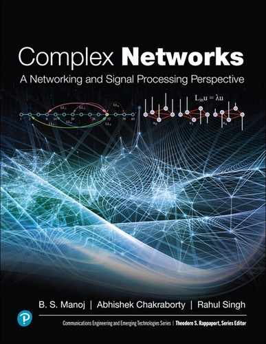
Graph signals are data values lying on the vertices of arbitrary graphs. An example graph signal is shown in Figure 9.1, where the vertical black lines going upward represent positive values and the black line going downward represents a negative value. Vertices of a graph represent entities, and the pairwise relationship between any two vertices is represented as an edge. A graph signal assigns a scalar value to each vertex based on some observations associated with the entities. For example, graph signals can be defined for temperatures within a geographical area, traffic capacities at hubs in a transportation network, or human behaviors in a social network. Graph signal processing (GSP) is concerned with modeling, representation, and processing of signals defined on graphs. Graph signal processing extends the concepts and tools that have been well developed in classical signal processing.

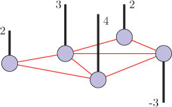
Figure 9.1. An example graph signal

In classical signal processing [159][160], we deal with discrete-time signals or image signals. An example of a discrete-time signal is shown in Figure 9.2(a). The vertical black lines represent corresponding strength of the signal samples at regular time instants t₁, t₂,... , t_N. A discrete-time signal can also be viewed as a signal lying on a regular structure that is a 1-D line graph, as shown in Figure 9.2(b). In this line graph, the nodes correspond to the time instants, and edges represent the time adjacency. In other words, the support of discrete-time signals is a regular line graph. Another class of signals that is considered in classical signal processing is image signals. A digital image contains rows and columns of pixels. Each pixel is assigned an intensity value to form an image signal. The image pixel lattice can be represented as an undirected graph that is a rectangular grid. Figure 9.3(a) shows an example image signal whose support is a 2-D rectangular grid, as shown in Figure 9.3(b). In this rectangular grid nodes correspond to the image pixels and the edges correspond to the pixel adjacency; that is, the pixels that are adjacent in space are connected by an edge. All the edge weights are assumed to be unity. Therefore, an image signal can be viewed as intensity values lying on a rectangular grid.

Two figures illustrating a discrete-time signal and its support.

Figure 9.2. A discrete-time signal and its support

An example of an image signal and its support is shown.

Figure 9.3. An example image signal and its support. Source: hannamariah/123RF.com

The support of discrete-time signals or image signals is unique and regular in nature: 1-D line graph for discrete-time signals and 2-D rectangular grid for image signals. Imagine signals supported on the structures shown in Figure 9.4, which are highly irregular in nature. For such signals, the classical signal processing techniques such as Fourier transform and wavelets cannot be applied because of the irregular nature of the underlying structure. Signals supported by these irregular structures, or graphs, are known as graph signals. The irregular support of graph signals is the main challenge for developing graph signal processing concepts. Many simple yet fundamental operations become extremely challenging when dealing with graph signals. The following difficulties may arise in the graph settings:

Illustrations of two examples of how graph signals are supported.

Figure 9.4. Example of supports of graph signals

The difficulty can be visualized from a very simple operation of translation. Translation operation is quite simple in classical settings. For example, to translate a signal left by 5 units, all the samples of the signal need to be advanced by 5 units. This operation is illustrated in Figure 9.5(a). In the figure, the solid curve represents the original signal, and the dashed curve represents the translated signal. However, if one wants to translate the graph signal shown in Figure 9.5(b) by, say, 1 unit, it is not straightforward. Since a node is connected to multiple nodes, it is not clear in which direction the sample value at the node should be moved. For example, node 5 is connected to nodes 2 and 4. To translate the sample value at node 5, should one move toward node 2 or node 4?

The graphs are placed one below the other and labeled alphabetically. Figure a shows the Time Shift in a graph plotted with values ranging from 0 to 20 the horizontal axis, and 0 to 12 along the vertical axis, both in increments of 2. The initial path in the graph is shown in blue. It begins at (0, 2) and proceeds as a line parallel to the horizontal axis until (6, 2). It is then traced through the following points, to resemble the outline of a house: (6, 2), (6, 4), (10, 12), (14, 4), and (14, 1). It ends in another parallel line from (14, 1) to (20, 1). The path of the graph after the time shift is shown in red dashes. A similar path is traced through the following points: (0, 2), (2, 2), (2, 4), (6, 16), (10, 4), (10, 1), (14, 1), and (20, 1). The parts of the graphs that run parallel to the horizontal axis overlap each other. Figure b pertains to the Translation of a graph signal that is not straight-forward. Five numbered nodes are present in the graph. Node 1 at the bottom-left is connected to node 2 and 3 diagonally above and below it to the right. Node 2 is connected to node 3 and to node 4, which is further to its right. Node 3 is connected to node 4. Node 5 is at the top and in-between nodes 2 and 4 and is connected to both. All connections are bi-directional. Vertical straight lines with varying magnitudes are drawn upward from the following nodes in the ascending order: 1, 5, 2, and 3. A vertical node is drawn downward from node 4 with a greater magnitude than the above four.

Figure 9.5. Illustration of translation
To downsample a discrete-time signal, alternate samples of the signal are discarded. However, to downsample the graph signal shown in Figure 9.1, which samples should be discarded?

Graph signal processing addresses these challenges by merging spectral graph theoretical concepts with computational harmonic analysis. The basic analogy between classical and graph signal processing is established through the eigenvalues and eigenvectors of graph Laplacian matrix, which carries a notion of frequency for graph signals and leads to the generalization of traditional signal processing techniques to the graph settings. For frequency analysis of graph signal analogous to classical Fourier transform, graph Fourier transform has been defined. Graph Fourier transform is not only useful in frequency analysis of graph signals, but has also been proved to be central in developing multiple concepts. For example, graph Fourier transform is used in constructing spectral graph wavelets that allow multiscale analysis of graph signals. Also, various operators such as convolution, translation, and modulation have been defined through graph Fourier transform. Throughout this chapter, we assume that the underlying graphs are undirected and have positive edge weights. The directed graphs will be considered in Chapter 10.

9.1.1 Mathematical Representation of Graph Signals

A graph is represented as G=(V,W) $? = (?, ?)$ , where V={v0,v1,…,vN−1} $? = {v_{0}, v_{1}, \dots, v_{N - 1}}$ is the set of vertices (or nodes) and W is the weight matrix of the graph in which an element w_ij represents the weight of the edge between nodes i and j (w_ij = 0, if there is no edge between nodes i and j). The size of the graph, N=|V| $N = | ? |$ , is the total number of nodes in the graph. A graph signal is a set of values defined on the vertices of the graph and it is represented as an N-dimensional vector f=[f(1),f(2),…,f(N)]T∈RN $? = [f (1), f (2), \dots, f (N)]^{T} \in ℝ^{N}$ , where f (i) is the value of the graph signal at node i. To store a graph signal in a computer, we need the weight matrix of the underlying structure and the signal vector.

9.2 Comparison between Classical and Graph Signal Processing

Classical signal processing is well equipped with a number of powerful tools and concepts that have been developed over several decades. Some of them include Fourier transform, filtering, convolution, translation, modulation, dilation, and windowed Fourier transform. Graph signal processing aims to extend these powerful concepts to data residing on general graphs.

The important tools and operators for classical and graph signal processing are summarized in Table 9.1. The concept of frequency analysis of the classical case is extended to the graph setting using eigendecomposition of the graph Laplacian matrix. Complex exponentials are used as expansion basis in classical Fourier transform, whereas in graph settings, eigenvectors of the graph Laplacian are used as expansion basis for graph signals. This equivalent transform in graph settings is termed as graph Fourier transform (GFT).

Table 9.1. Classical vs. graph signal processing

Operator/Transform	Classical Signal Processing	Graph Signal Processing
Fourier Transform	∙ $•$ xˆ(ω)=∫∞−∞x(t)e−jωtdt $\hat{x} (ω) = \int_{- \infty}^{\infty} x (t) e^{- j ω t} d t$ • Frequency: ω can take any real value • Fourier basis: Complex exponentials e^jωt	∙ $•$ fˆ(λℓ)=∑Nn=1f(n)u∗ℓ(n) $\hat{?} (λ_{ℓ}) = \sum_{n = 1}^{N} ? (n) ?_{ℓ}^{} (n)$ • Frequency: Eigenvalues of the graph Laplacian (λ_ℓ*) • Fourier basis: Eigenvectors of the graph Laplacian (u_ℓ)
Convolution	• In time domain: x(t)y(t)=∫∞−∞x(τ)y(t−τ)dτ $x (t) y (t) = \int_{- \infty}^{\infty} x (τ) y (t - τ) d τ$ • In frequency domain: x(t)y(t)ˆ=xˆ(ω)yˆ(ω) $\hat{x (t) y (t)} = \hat{x} (ω) \hat{y} (ω)$	• Defined through graph Fourier transform ∙ $•$ fgˆ=(fˆ⊙gˆ) $\hat{? ?} = (\hat{?} ⊙ \hat{?})$
Translation	• Can be defined using convolution • T_τ x(t) = x(t − τ) = x(t) ∗ δ_τ(t)	• Defined through graph convolution ∙ $•$ (Tif)(n)=N−−√(fδi)(n)=N−−√∑N−1ℓ=0fˆ(λℓ)u∗ℓ(i)uℓ(n) $(T_{i} ?) (n) = \sqrt{N} ({f δ}_{i}) (n) = \sqrt{N} \sum_{ℓ = 0}^{N - 1} \hat{f} (λ_{ℓ}) u_{ℓ}^{*} (i) u_{ℓ} (n)$
Modulation	• Multiplication with the complex exponential • M_ω x(t) = e^jωt x(t)	• Multiplication with the eigenvector of the graph Laplacian ∙ $•$ (Mkf)(n)=N−−√uk(n)f(n) $(M_{k} ?) (n) = \sqrt{N} u_{k} (n) f (n)$
Windowed Fourier Transform	• Defined through translation and modulation of a window	• Generalized translation and modulation operators are used

The convolution product of two graph signals is defined through GFT. This analogy is drawn from the well-known classical convolution theorem according to which convolution in the time domain is equivalent to multiplication in the frequency domain.

Translating a classical signal is equivalent to convoluting the signal with an impulse. Similarly, a translation operator in graph settings has been defined through convolution product with an impulse.

In classical signal processing, modulation of a signal to a certain frequency is nothing but multiplication of the signal with the complex exponential at that frequency. Similarly, the modulation operator in a graph setting is achieved through multiplication of the eigenvector of the graph Laplacian.

9.2.1 Relationship between GFT and Classical DFT

Discrete Fourier transform (DFT) of a discrete-time signal x∈CN $? \in ℂ^{N}$ can be calculated as xˆ=Tx $\hat{?} = ? ?$ is the transformation DFT matrix. The DFT matrix is

(9.2.1) T=DFTN=⎡⎣⎢⎢⎢⎢⎢⎢⎢⎢⎢⎢⎢⎢⎢⎢⎢⎢1111⋮11e−2πjNe−2πjN2e−2πjN3⋮e−2πjN(N−1)1e−2πjN2e−2πjN4e−2πjN6e−2πjN2(N−1)1e−2πjN3e−2πjN6e−2πjN9e−2πjN3(N−1)……⋱…1e−2πjN(N−1)e−2πjN2(N−1)e−2πjN3(N−1)⋮e−2πjN(N−1)(N−1)⎤⎦⎥⎥⎥⎥⎥⎥⎥⎥⎥⎥⎥⎥⎥⎥⎥⎥. $? = {? ? ?}_{N} = [\begin{matrix} 1 & 1 & 1 & 1 & \dots & 1 \\ 1 & e^{- \frac{2 π j}{N}} & e^{- \frac{2 π j}{N} 2} & e^{- \frac{2 π j}{N} 3} & \dots & e^{- \frac{2 π j}{N} (N - 1)} \\ 1 & e^{- \frac{2 π j}{N} 2} & e^{- \frac{2 π j}{N} 4} & e^{- \frac{2 π j}{N} 6} & e^{- \frac{2 π j}{N} 2 (N - 1)} \\ 1 & e^{- \frac{2 π j}{N} 3} & e^{- \frac{2 π j}{N} 6} & e^{- \frac{2 π j}{N} 9} & e^{- \frac{2 π j}{N} 3 (N - 1)} \\ ⋮ & ⋮ & ⋱ & ⋮ \\ 1 & e^{- \frac{2 π j}{N} (N - 1)} & e^{- \frac{2 π j}{N} 2 (N - 1)} & e^{- \frac{2 π j}{N} 3 (N - 1)} & \dots & e^{- \frac{2 π j}{N} (N - 1) (N - 1)} \end{matrix}] .$

A classical discrete-time periodic signal can be viewed as a graph signal living on a ring graph, as shown in Figure 9.6. The Laplacian matrix of a ring graph is a circulant matrix (see Appendix A.2.4 for details) and can be written as and one possible choice of the corresponding (complex) eigenvectors is¹

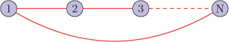
Figure 9.6. A ring graph: support of a discrete-time signal

(9.2.2) L=⎡⎣⎢⎢⎢⎢⎢⎢⎢⎢⎢⎢2−10⋮0−1−12−1000−1200…⋱0002−1−100⋮−12⎤⎦⎥⎥⎥⎥⎥⎥⎥⎥⎥⎥. $? = [\begin{matrix} 2 & - 1 & 0 & \dots & 0 & - 1 \\ - 1 & 2 & - 1 & 0 & 0 \\ 0 & - 1 & 2 & 0 & 0 \\ ⋮ & ⋱ & ⋮ \\ 0 & 0 & 0 & 2 & - 1 \\ - 1 & 0 & 0 & - 1 & 2 \end{matrix}] .$

The eigenvalues of the graph Laplacian of an N-node ring graph are

λℓ=2−2cos(2πℓN),∀ℓ={0,1,…,N−1} $λ_{ℓ} = 2 - 2 c o s (\frac{2 π ℓ}{N}), \forall ℓ = {0, 1, \dots, N - 1}$

uℓ=1N√⎡⎣⎢⎢⎢⎢⎢⎢⎢⎢⎢1e2πjNℓe2πjN2ℓ⋮e2πjN(N−1)ℓ⎤⎦⎥⎥⎥⎥⎥⎥⎥⎥⎥,∀ℓ={0,1,…,N−1}. $?_{ℓ} = \frac{1}{\sqrt{N}} [\begin{matrix} 1 \\ e^{\frac{2 π j}{N} ℓ} \\ e^{\frac{2 π j}{N} 2 ℓ} \\ ⋮ \\ e^{\frac{2 π j}{N} (N - 1) ℓ} \end{matrix}], \forall ℓ = {0, 1, \dots, N - 1} .$

These eigenvectors are nothing but the columns of the DFT matrix given by Equation 9.2.1. Therefore, classical discrete-time Fourier basis are eigenvectors of the Laplacian of the undirected ring graph.

9.3 The Graph Laplacian as an Operator

As discussed in Chapter 2, the Laplacian matrix of a graph is defined as

(9.3.1) L=D−W, $? = ? - ?,$

where D is the degree matrix and W is the weight matrix of the graph. For a graph signal f∈RN $? \in ℝ^{N}$ , the Laplacian operator satisfies

(9.3.2) (Lf)(i)=∑j∈Viwji[f(i)−f(j)], $(??) (i) = \sum_{j \in ?_{i}} w_{j i} [f (i) - f (j)],$

where Vi $?_{i}$ is the set of vertices connected to node i via an edge. Therefore, when operated on by the Laplacian operator, the value of a graph signal at node i is replaced by the weighted sum of the differences between the value at node i and the values at the adjacent nodes.

9.3.1 Properties of the Graph Laplacian

The graph Laplacian constitutes some importantpropertiesthatmakeitextremely useful in the analysis of graph signals. Properties of the Laplacian matrix that are utilized in graph signal processing are listed below. Note that the underlying graph is assumed to be undirected with positive edge weights.

The Laplacian matrix is symmetric.
The eigenvalues and eigenvectors of the Laplacian matrix are real. The symmetric nature of the Laplacian results in this property.
The Laplacian matrix is positive semidefinite; that is, all the eigenvalues of the Laplacian are greater than or equal to zero. It holds true only for graphs with positive edge weights.
The Laplacian matrix always has at least one zero eigenvalue. Moreover, for connected graphs it has only one zero eigenvalue. This property results from the fact that all the rows of the Laplacian matrix sum to zero, thereby ensuring at least one zero eigenvalue.
It has a complete set of orthonormal eigenvectors; that is, it forms a complete orthonormal basis.

The eigenvalues and eigenvectors of the graph Laplacian provide means for analyzing graph signals in the frequency domain, and thus make the graph Laplacian the basic building block of graph signal processing. Although the properties of eigenvalues and eigenvectors of the graph Laplacian have been extensively studied for the analysis of graph structure [161], [162], graph signal processing utilizes the oscillations of eigenvectors of the Laplacian matrix for analyzing signals defined on graphs.

Use of the graph Laplacian for frequency analysis of graph signals is limited to signals residing on undirected graphs. The primary advantage of using graph Laplacian for frequency analysis is that it results in simple analysis and gives precise analogy to classical signal processing. Another framework that uses directed Laplacian for analyzing data residing on directed graphs is discussed in Chapter 10.

9.3.2 Graph Spectrum

The set of eigenvalues of the graph Laplacian matrix is known as graph spectrum or Laplacian spectrum (of graphs). Graph Laplacian L is a real symmetric matrix, and it has a complete set of orthonormal eigenvectors [163]. L is also a positive semidefinite matrix; therefore, it has nonnegative eigenvalues. Moreover, for connected graphs, the multiplicity of zero eigenvalue is one. We denote the system of eigenvalues and eigenvectors of L as L as ${λ_{ℓ}, ?_{ℓ}}_{ℓ = 0}^{N - 1}$ , where λ_ℓ is the eigenvalue of L and u_ℓ is the corresponding eigenvector. The graph spectrum of an N-node graph $?$ is represented as $σ (?) = {λ_{0}, λ_{1}, \dots, λ_{N - 1}}$ , where 0 = λ₀ ≤ λ₁ ≤ λ₂ ··· ≤ λ_N₋₁.

9.4 Quantifying Variations in Graph Signals

In classical signal processing, smoothness means adjacent signal coefficients have similar values. The concept of smoothness is useful in numerous applications. A widely used application is denoising; to eliminate noise from a corrupted a signal, the noisy signal is smoothened by using an averaging filter to remove noise. Gradient measures and total variation are some of the popular measures of smoothness (or variation) in classical signal processing. These concepts can easily be extended to graph settings.

Smoothness of a graph signal is defined with respect to the intrinsic structure of the weighted graph on which signal values lie. Smoothness of a graph signal with respect to the structure of the underlying graph is quantified using some discrete differential operators such as edge derivative and gradient.

The edge derivative of a graph signal f with respect to edge e_ij (which connects the vertices i and j) at vertex i is defined as

(9.4.1) ${\frac{\partial ?}{\partial e_{i j}} |}_{i} = \sqrt{w_{i j}} [f (j) - f (i)]$

and the graph gradient of the signal f at vertex i is the N-dimensional vector containing all the edge derivatives at vertex i:

(9.4.2) $\nabla_{i} ? = {{\frac{\partial ?}{\partial e_{i j}} |}_{i}}_{j \in ?} .$

Note that the number of non-zero entries in the gradient vector at node i is the number of nodes connected to the node i.

The local variation of the signal f at vertex i is expressed as the ℓ₂-norm of the gradient vector at node i:

(9.4.3) $\begin{matrix} ∥ \nabla_{i} f ∥_{2} & = {[\underset{j \in ν_{i}}{Σ} {(\frac{\partial f}{\partial e_{i j}})}^{2}]}^{\frac{1}{2}} \\ = {[\underset{j \in ν_{i}}{Σ} w_{i j} {[f (j) - f (i)]}^{2}]}^{\frac{1}{2}} . \end{matrix}$

where $?_{i}$ is the set of vertices that are connected to the vertex i. Local variation provides a measure of local smoothness of f around vertex i, as it is small when the function f has similar values at i and all neighboring vertices of i.

For measuring global smoothness, the discrete p-Dirichlet form (S_p(f)) of f can be used, which is defined as

(9.4.4) $S_{p} (f) = \frac{1}{p} \underset{i \in ν}{Σ} ∥ \nabla_{i} f ∥_{2}^{p} = \frac{1}{p} \underset{i \in ν}{Σ} {[\underset{i \in ν_{i}}{Σ} w_{i j} {[f (j) - f (i)]}^{2}]}^{\frac{p}{2}}$

For p = 1, S₁(f) is known as total variation of the graph signal with respect to the graph. Therefore, total variation can be written as

(9.4.5) $T V (f) = S_{1} (f) = \underset{i \in ν}{Σ} ∥ \nabla_{i} f ∥_{2} = \underset{i \in ν}{Σ} {[\underset{i \in ν_{i}}{Σ} w_{i j} {[f (j) - f (i)]}^{2}]}^{\frac{1}{2}}$

For p = 2, we have

(9.4.6) $\begin{matrix} S_{2} (f) & = \frac{1}{2} \underset{i \in ν}{Σ} \underset{i \in ν_{i}}{Σ} w_{i j} {[f (j) - f (i)]}^{2} \\ = \underset{i, j \in ϵ}{Σ} w_{i j} {[f (j) - f (i)]}^{2} = f^{T} L f . \end{matrix}$

Therefore, S₂(f) is also known as the graph Laplacian quadratic form. When the signal f has similar values at neighboring vertices connected by an edge with a large weight—that is, when it is smooth—then S₂(f) has a small value. Thus, the smoothness not only depends on the signal values but also depends on the underlying graph structure. The Laplacian quadratic form or 2-Dirichlet form can be used to order the graph frequencies (Section 9.5.1), interpolation on graphs,² and denoising of noisy graphs signals. The values of graph Laplacian quadratic form of the Laplacian eigenvectors associated with lower eigenvalues are small as compared to the Laplacian eigenvectors associated with higher eigenvalues.

9.5 Graph Fourier Transform

Consider a graph signal f = [2, 3, 2, −3, 4]^T shown in Figure 9.1. This signal can be alternatively represented as a linear combination of certain graph signals as

$\begin{matrix} ? = & [\begin{matrix} 2 \\ 3 \\ 2 \\ - 3 \\ 4 \end{matrix}] = (?.??) [\begin{matrix} 0.45 \\ 0.45 \\ 0.45 \\ 0.45 \\ 0.45 \end{matrix}] + (?.??) [\begin{matrix} 0.60 \\ 0.37 \\ 0 \\ - 0.37 \\ - 0.60 \end{matrix}] + (?.??) [\begin{matrix} 0.51 \\ - 0.20 \\ - 0.63 \\ - 0.20 \\ 0.51 \end{matrix}] \\ + (-?.??) [\begin{matrix} 0.37 \\ - 0.60 \\ 0 \\ 0.60 \\ - 0.37 \end{matrix}] + (?.??) [\begin{matrix} 0.20 \\ - 0.51 \\ 0.63 \\ - 0.51 \\ 0.20 \end{matrix}] . \end{matrix}$

The constituent graph signals in the above sum are nothing but the eigenvectors of the graph Laplacian. These graph signals are known as the graph harmonics. What are the advantages in such a representation? What interesting information do we get from the coefficients of the graph harmonics in the sum? The eigenvectors of the graph Laplacian have a notion of frequency, and the coefficients in the above sum are known as GFT coefficients. The GFT is analogous to the classical Fourier transform and is extremely useful in analyzing graph signals.

The classical Fourier transform allows frequency analysis of discrete-time and image signals, and it lies at the heart of classical signal processing. It decomposes a signal as a linear combination of complex exponentials, which provides notion of frequency. Analogous to the classical Fourier transform, the GFT extends the notion of frequency to irregular graph settings. It provides us a means to extract the structural properties of a graph signal that are not visible in the vertex domain and become evident in the transform (frequency) domain. In graph settings, the notion of frequency is derived from the eigendecomposition of the graph Laplacian matrix. The eigenvalues of the graph Laplacian act as graph frequencies, and the eigenvectors of the graph Laplacian act as graph Fourier basis. It is important to note that the classical Fourier bases are fixed, however, graph Fourier bases depend on the network topology and change with the network structure.

Classical Fourier transform decomposes a signal as a linear combination of complex exponentials known as the Fourier basis. The classical Fourier transform of a function x(t) is given by

(9.5.1) $\hat{x} (ω) = \int_{- \infty}^{\infty} x (t) e^{- j ω t} d t,$

where ω is the angular frequency (in radians per second). For large values of ω, the oscillations of complex exponentials e^jωt with respect to time t are rapid, and vice versa. Therefore, large values of ω correspond to high frequencies and small values of ω correspond to low frequencies. Furthermore, these complex oscillations are also the eigenfunctions of 1-D Laplace operator Δ, because

(9.5.2) $- Δ (e^{j ω t}) = - \frac{\partial^{2}}{\partial t^{2}} e^{j ω t} = (ω)^{2} e^{j ω t} .$

Drawing the analogy from the fact that the complex exponentials are the eigenfunctions of the 1-D Laplace operator, the eigenvectors of the graph Laplacian can be used as a graph Fourier basis. Therefore, the GFT $\hat{?}$ of a graph signal f can be defined as the expansion of f in terms of the eigenvectors of the graph Laplacian:

(9.5.3) $\hat{f} (λ_{ℓ}) = ⟨ f, u_{ℓ} ⟩ = Σ_{n = 1}^{N} f (n) u_{ℓ}^{*} (n),$

where $\hat{f} (λ_{ℓ})$ is the GFT coefficient corresponding to eigenvalue λ_ℓ and $u_{ℓ}^{*} (n)$ is the complex conjugate of u_ℓ(n). 〈f₁, f₂〉 denotes the inner product of vectors f₁ and f₂. The eigenvectors of the graph Laplacian act as graph harmonics similar to complex exponentials in the classical Fourier transform. The inverse graph Fourier transform (IGFT) is given by

(9.5.4) $f (n) = Σ_{ℓ = 0}^{N - 1} \hat{f} (λ_{ℓ}) u_{ℓ} (n) .$

The set of GFT coefficients of a graph signal is called the spectrum of the graph signal. By using GFT in Equation (9.5.3) and IGFT in Equation (9.5.4) a graph signal is represented equivalently in two different domains: the vertex domain and the graph spectral domain. GFT is an energy preserving transform, and a signal can be considered as low-pass (or high-pass) if the energy of the GFT coefficients of that signal are mostly concentrated on the low-pass (or high-pass) eigenvectors.

To define GFT and IGFT in matrix form, consider U = [u₀|u₁| ... |u_N₋₁] to be the matrix whose columns are the eigenvectors of L. Then the GFT of a graph signal f can be expressed as

(9.5.5) $\hat{?} = ?^{T} ? .$

In the transformed vector $\hat{?} = [\hat{f} (λ_{0}) \hat{f} (λ_{1}) \dots \hat{f} (λ_{N - 1})]^{T}$ , $\hat{f} (λ_{ℓ}) = ⟨ ?, ?_{ℓ} ⟩$ is the GFT coefficient corresponding to eigenvalue λ_ℓ. Moreover, IGFT can be calculated as

(9.5.6) $? = ? \hat{?} .$

As an example to illustrate GFT, consider the graph signal shown in Figure 9.7(a). The corresponding GFT coefficients with respect to the graph frequencies are plotted in Figure 9.7(b), where the horizontal axis represents the graph frequencies (the eigenvalues of the graph Laplacian) and the vertical axis represents the magnitude of the GFT coefficients. As another example, consider a heat kernel defined on the Minnesota road network. In the graph spectral domain, the heat kernel is represented as $\hat{g} (λ_{ℓ}) = e^{- 2 λ_{ℓ}}$ , as shown in Figure 9.8(a). The vertex domain representation of the heat kernel is depicted in Figure 9.8(b).

Two figures showing a graph Fourier transform.

The two figures are placed side-by-side and labeled alphabetically. Figure a pertains to a graph signal f. There are five nodes in the graph, such that four nodes form a rhombus and the fifth node is positioned centrally above them. The nodes forming the rhombus are connected in a ring and the top-left and bottom-right nodes are connected diagonally. The fifth node above is connected to the two nodes diagonally below it to the left and right. The color of the nodes vary in shades of brown, and a gradient scale beside reads that the lightest corresponds to -2, followed by 0, 2, and the darkest at 4. Figure b is a graph marked with lambda subscript l values from 0 to 4 in increments of 1 along the horizontal axis and f circumflex (lambda subscript l) values from -4 to 2 in increments of 2 along the vertical axis. A straight line runs parallel to the horizontal axis from the point 0 along the vertical axis. The following vertical lines are drawn from this line: (0, 0) to (0, 6), (0.5, 0) to (0.5, 1), (1.3, 0) to (1.3, 2), (2.6, 0) to (2.6, -4), and (3.6, 0) to (3.6, 2.4).

Figure 9.7. Example of graph Fourier transform: a graph signal in vertex and frequency domains

The different representations of the kernel in spectral and vertex domains.

The first figure is labeled a and pertains to the Heat kernel g circumflex (lambda subscript l) equals e to the power of (-2 times lambda subscript l) in graph spectral domain. It is a graph with lambda subscript l values on the horizontal axis from 0 to 7 in increments of 1 and g circumflex (lambda subscript l) values ranging from 0.2 to 1 in increments of 0.2 along the vertical axis. A straight line is drawn from (0, 0) to (0, 1). From (0, 1), a curve drops gradually and approaches the horizontal axis. It then travels parallel to the horizontal axis until (7, 0). The area bounded by the first straight line, the curve and the horizontal axis is shaded. The second figure b shows the kernel in the vertex domain. Here a number of nodes are present along with their magnitude lines extended either from above or below it. The nodes are interconnected densely. The third figure c shows another representation of the kernel in the vertex domain. Here also there are several nodes interconnected. The nodes at the bottom are more densely connected. The nodes vary in shades of grey and a scale to the right read that the lightest shade pertains to 0, followed by 2, and the darkest at 4.

Figure 9.8. Representation of the kernel in spectral and vertex domains

GFT gives frequency content present in a signal defined on a graph. However, it does not reveal local properties of a graph signal. It tells us what frequency components are present in a graph signal, but it does not tell us where in space these frequency components are present. To find out where in space the frequency content are present, one can use windowed graph Fourier transform (WGFT), discussed in Section 9.8. Moreover, to localize graph signal content in the vertex and spectral domains simultaneously, spectral graph wavelet transform (SGWT), discussed in Chapter 11, can be used.

The GFT defined above is applicable to an undirected graph with nonnegative edge weights. There exist other definitions of GFT that are applicable to directed graphs with negative or complex weights as well. These approaches are described in Chapter 10.

9.5.1 Notion of Frequency and Frequency Ordering

The eigenvalues and eigenvectors of the graph Laplacian provide a notion of frequency. The eigenvectors act as natural vibration modes of the graph, and the corresponding eigenvalues act as associated graph frequencies. Eigenvalue 0 corresponds to zero frequency, and the associated eigenvector u₀ is constant and has a value of $1 / \sqrt{N}$ at each node [163]. The eigenvalues of the graph shown in Figure 9.7(a) are {0, 0.38, 1.38, 2.62, 3.62} and the corresponding eigenvector matrix is

(9.5.7) $? = [?_{0} \dots ?_{4}] = [\begin{matrix} 0.45 & 0.60 & - 0.51 & 0.37 & 0.20 \\ 0.45 & 0.37 & - 0.20 & - 0.60 & - 0.51 \\ 0.45 & 0 & - 0.63 & 0 & 0.63 \\ 0.45 & - 0.37 & - 0.20 & 0.60 & - 0.51 \\ 0.45 & - 0.60 & 0.51 & - 0.37 & 0.20 \end{matrix}] .$

The notion of frequency in the eigenvectors of the graph Laplacian can be visualized through the relation between zero crossings and frequency. Consider the discrete-time signals shown in Figure 9.9. What can be concluded about the frequency content of each of these signals? The first signal does not change with time, or in other words, it has no zero crossings. There is one zero crossing if adjacent signal sample values change their sign, that is, if the signal values go positive from negative or negative from positive. The signal shown in Figure 9.9(b) is a slowly varying signal. There are a few zero crossings; that is, the signal has dominating low frequencies. However, the signal shown in Figure 9.9(c) changes rapidly and has a large number of zero crossings. It suggests that the signal contains significant high frequencies. Therefore, it can be argued that more zero crossings correspond to high frequencies. This relation between zero crossings and frequency can be extended to graph signals too. The eigenvectors of the Laplacian matrix of the graph are plotted in Figure 9.10. Figure 9.10(a) shows the eigenvector corresponding to zero eigenvalue. It has a constant value at each node of the graph, suggesting zero frequency. With the increase in eigenvalue, the zero crossings in the corresponding eigenvector increase, which indicates increase in frequency too. However, by observing zero crossings in a graph signal, only a vague idea regarding its frequency contents can be made. Therefore, some parameter is needed to quantify the oscillations in graph signals and subsequently to order the graph frequencies accurately. Various parameters, such as total variation and p-Dirichlet defined in the previous section, can be used to quantify the oscillations or variations in the graph Fourier basis for the purpose of frequency ordering.

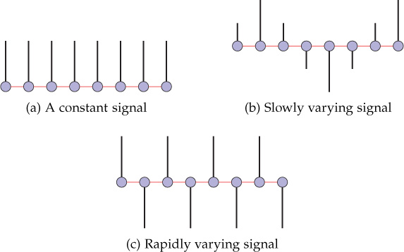
The diagrammatic illustrations of discrete-time signals with various frequencies.

Figure 9.9. Discrete-time signals with various frequencies

The Eigenvectors of a Laplacian graph are displayed.

There are five figures labeled alphabetically. The described graph is present in all the figures. Five nodes are present in the graph such that the leftmost node 1, is connected to two nodes to its top and bottom right, namely 2 and 3. These two nodes are connected to each other. Two other nodes 4 and 5, are present further on the right of nodes 2 and 3. The following nodes are connected: 2 to 4 and 5, 3 to 5, and 4 to 5. Figure a corresponds to u subscript 0, wherein all nodes have vertical lines extended from their top with an equal magnitude. The value written beside node 1 is 0.45. Figure b corresponds to u subscript 1, wherein vertical lines are extended from the top of nodes 1, 2, and 3, and from the bottom of nodes 4 and 5, with varying magnitudes. The value written beside node 1 is 0.60. Figure c corresponds to u subscript 2, wherein vertical lines are extended from the top of nodes 1, 3, and 5, and from the bottom of nodes 2 and 4, with varying magnitudes. The value written beside node 1 is 0.51. Figure d corresponds to u subscript 3, wherein vertical lines are extended from the top of nodes 1, 3, and 4, and from the bottom of nodes 2 and 5, with varying magnitudes. The value written beside node 1 is 0.37. Figure e corresponds to u subscript 4, wherein vertical lines extended from the top of nodes 1, 3, and 5, and from the bottom of nodes 2 and 4, with varying magnitudes. The value written beside node 1 is 0.20.

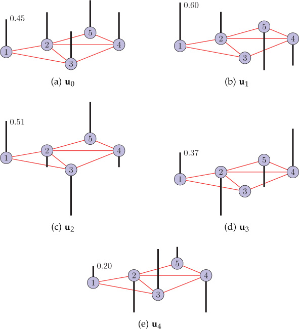
Figure 9.10. Eigenvectors of the graph Laplacian

Generally, 2-Dirichlet form or graph Laplacian quadratic form is used for the purpose of frequency ordering. The graph Laplacian quadratic form of the Laplacian eigenvectors is shown in Table 9.2. The graph Laplacian quadratic form of an eigenvector is equal to the corresponding eigenvalue, since $?_{ℓ}^{T} {? ?}_{ℓ} = ?_{ℓ}^{T} λ_{ℓ} ?_{ℓ} = λ_{ℓ}$ . Therefore, the eigenvector corresponding to a small eigenvalue has low value of graph Laplacian quadratic form, and vice versa, and thus results in the natural order of frequency–small eigenvalues correspond to low frequency, and vice versa. Frequency ordering is visualized in Figure 9.11.

Table 9.2. Laplacian quadratic forms of the Laplacian eigenvectors of the graph shown in Figure 9.7

Eigenvectors	Eigenvalues	Graph Laplacian Quadratic Form
u₀ = [0.45 0.45 0.45 0.45 0.45]^T	0	0
u₁ = [0.60 0.37 0 − 0.37 − 0.60]^T	0.38	0.38
u₂ = [−0.51 − 0.20 − 0.63 − 0.20 0.51]^T	1.38	1.38
u₃ = [0.37 − 0.60 0 0.60 − 0.37]^T	2.62	2.62
u₄ = [0.20 − 0.51 0.63 − 0.51 0.20]^T	3.62	3.62

Figure 9.11. Frequency ordering from low frequencies to high frequencies. As one moves away from the zero eigenvalue to higher eigenvalues, the eigenvalues correspond to higher frequencies.

From the above discussion, it can be concluded that the eigenvectors of the Laplacian matrix corresponding to low frequencies are smooth with respect to the graph—they vary slowly across the graph. That is, if an edge with a large weight connects two vertices, the values of the eigenvector at those nodes are likely to be similar. The eigenvectors corresponding to larger eigenvalues vary more rapidly as we move from one node to other adjacent node connected by an edge with large weight. Therefore, the eigenvalues of graph Laplacian matrix carry the notion of frequency, where smaller eigenvalues correspond to low frequencies and larger eigenvalues correspond to high frequencies. It should be noted that the graph frequencies are specific to a particular graph. The frequency values cannot be compared between different graphs. For example, consider a graph $?_{1}$ having frequencies 0, 0.1, 0.2, 0.3, and 1.2, and a graph $?_{2}$ having frequencies 0, 1.2, 2.6, 2.8, and 3. Here, the frequency value of 1.2 corresponds to high frequency for $?_{1}$ but corresponds to low frequency for $?_{2}$ . Indeed, a small change in the topology of a network, resulting from perturbations such as removal or addition of a few edges, changes the graph spectrum completely.

Example

This example illustrates the GFT of an impulse defined on a graph. An impulse δ_i is a graph signal having all zero values except unit value at node i. In other words,

(9.5.8) $?_{i} (n) = {\begin{matrix} 1 & if n = i \\ 0 & otherwise . \end{matrix}$

A graph signal can be represented as a linear combination of impulses. Let ${?'}_{i} = ?^{T} (:, i)$ :

(9.5.9) ${?'}_{i} = [\begin{matrix} ?_{0} (i) \\ ?_{1} (i) \\ ?_{2} (i) \\ ⋮ \\ ?_{N - 1} (i) \end{matrix}] .$

Therefore, GFT of an impulse at node i is

(9.5.10) ${\hat{?}}_{i} = ?^{T} ?_{i} = {?'}_{i} .$

Figure 9.12 shows an impulse at node 3 of the graph. The eigenvector matrix of the graph is

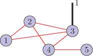
A diagrammatic representation of an impulse on a graph.

Figure 9.12. Impulse on a graph (δ₃)

$? = [?_{0} ?_{1} ?_{2} ?_{3}] = [\begin{matrix} 0.4472 & 0.4375 & 0.7031 & 0 & 0.3380 \\ 0.4472 & 0.2560 & - 0.2422 & 0.7071 & - 0.4193 \\ 0.4472 & 0.2560 & - 0.2422 & - 0.7071 & - 0.4193 \\ 0.4472 & - 0.1380 & - 0.5362 & 0 & 0.7024 \\ 0.4472 & - 0.8115 & 0.3175 & 0 & - 0.2018 \end{matrix}] .$

The GFT of the impulse δ₃ is

(9.5.11) ${\hat{?}}_{3} = {?'}_{3} = [\begin{matrix} 0.4472 \\ 0.2560 \\ - 0.2422 \\ - 0.7071 \\ - 0.4193 \end{matrix}] .$

9.5.2 Bandlimited Graph Signals

A graph signal is said to be bandlimited to a graph frequency $ω \in ℝ$ , if the GFT coefficients of the signal are zero outside the graph frequency band [0, ω]. The graph frequency ω is known as bandwidth of the signal. Therefore, for an ω-bandlimited signal f,

(9.5.12) $\hat{f} (λ_{ℓ}) = 0 \forall λ_{ℓ} > ω .$

The space of ω-bandlimited signals is known as Paley-Wiener space [164]. The Paley-Wiener space is a subspace of $ℝ^{N}$ and is denoted by $P V_{ω} (?)$ .

9.5.3 Effect of Vertex Indexing

Suppose we are given the values of a graph signal attached to every vertex of the graph. What will happen if only vertex indexing is changed (while keeping all other parameters unchanged)? Figure 9.13(a) shows a weighted graph, and Figure 9.13(b) shows a graph signal defined on the graph of 9.13(a). If only the vertex indexing is changed, as in Figure 9.13(c), how will the signal representation change in the vertex and frequency domains?

Four graphs with different vertex indexing are displayed.

The figures are placed two in a row and labeled alphabetically. Figure a shows an example graph G1. Four nodes are present at the four vertices of an imaginary kite. The nodes are labeled 1, 2, 3, and 4 in a clockwise manner, such that the leftmost node is 1. The following nodes are connected with the corresponding values written across each connection: 1 and 2 with 0.3, 1 and 3 with 0.1, 2 and 3 with 0.2, 2 and 4 with 0.5, and 3 and 4 with 0.7. Figure b shows a graph signal defined on G1: f1 = [5, 2, 6, 9] superscript T. The graph in figure a is shown tilted to its right, such that the kite now seems to be resting flat. Vertical lines are extended from the top of every node with the following magnitude values written beside each respectively: 5, 2, 6, and 9. The length of each vertical line corresponds to that of its magnitude. Figure c shows a graph G2 with a different vertex indexing. The graph is similar to figure a, except that the nodes shift position to the right. Hence node 1 is the now the topmost node. The connections and values corresponding to each connection are the same. Figure d is labeled to be a graph signal defined on G2: f2 = [2, 6, 9, 5] superscript T. The graph in figure c is shown tilted to its right, such that the kite now seems to be resting flat. Vertical lines are extended from the top of every node with the following magnitude values written beside each respectively: 2, 6, 9, and 5.

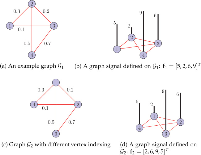
Figure 9.13. Graphs with different vertex indexing

First consider the graph $?_{1}$ shown in Figure 9.13(a). Its Laplacian and the corresponding eigenvector matrix are

(9.5.13) $?_{1} = [\begin{matrix} 0.4 & - 0.3 & - 0.1 & 0 \\ - 0.3 & 1 & - 0.2 & - 0.5 \\ - 0.1 & - 0.2 & 1 & - 0.7 \\ 0 & - 0.5 & - 0.7 & 1.2 \end{matrix}] ?_{1} = [\begin{matrix} 0.5 & 0.8316 & 0.2185 & 0.1034 \\ 0.5 & - 0.0494 & - 0.7942 & - 0.3417 \\ 0.5 & - 0.3837 & 0.5669 & - 0.5305 \\ 0.5 & - 0.3985 & 0.0088 & 0.7689 \end{matrix}] .$

The graph signal f₁ = [5, 2, 6, 9]^T (Figure 9.13(b)) can be represented as the linear combination of eigenvectors of the graph Laplacian:

$\begin{matrix} ?_{1} & = [\begin{matrix} 5 \\ 2 \\ 6 \\ 9 \end{matrix}] \\ = (11) [\begin{matrix} 0.5 \\ 0.5 \\ 0.5 \\ 0.5 \end{matrix}] + (- 1.83) [\begin{matrix} 0.8316 \\ - 0.0494 \\ - 0.3837 \\ - 0.3985 \end{matrix}] + (2.98) [\begin{matrix} 0.2185 \\ - 0.7942 \\ 0.5669 \\ 0.0088 \end{matrix}] + (3.57) [\begin{matrix} 0.1034 \\ - 0.3417 \\ - 0.5305 \\ 0.7689 \end{matrix}] . \end{matrix}$

Therefore, ${\hat{?}}_{1} = [11, - 1.83, 2.98, 3.57]^{T}$ .

Now consider the graph $?_{2}$ in Figure 9.13(c), which is the same as the original graph (Figure 9.13(a)) except for a different vertex indexing. The Laplacian and the eigenvector matrix of this graph are

(9.5.14) $?_{2} = [\begin{matrix} 1 & - 0.2 & - 0.5 & - 0.3 \\ - 0.2 & 1 & - 0.7 & - 0.1 \\ - 0.5 & - 0.7 & 1.2 & 0 \\ - 0.3 & - 0.1 & 0 & 0.4 \end{matrix}] ?_{2} = [\begin{matrix} 0.5 & - 0.0494 & - 0.7942 & - 0.3417 \\ 0.5 & - 0.3837 & 0.5669 & - 0.5305 \\ 0.5 & - 0.3985 & 0.0088 & 0.7689 \\ 0.5 & 0.8316 & 0.2185 & 0.1034 \end{matrix}]$

Altering just the vertex indexing in the graph signal f₁ results in a corresponding indexing change in the signal. The resulting graph signal in the vertex domain is represented as f₂ = [2, 6, 9, 5]^T which is shown in Figure 9.13(d). It can be written as the linear combination of eigenvectors of the graph Laplacian:

$\begin{matrix} ?_{2} & = [\begin{matrix} 2 \\ 6 \\ 9 \\ 5 \end{matrix}] \\ = (11) [\begin{matrix} 0.5 \\ 0.5 \\ 0.5 \\ 0.5 \end{matrix}] + (- 1.83) [\begin{matrix} - 0.0494 \\ - 0.3837 \\ - 0.3985 \\ 0.8316 \end{matrix}] + (2.98) [\begin{matrix} - 0.7942 \\ 0.5669 \\ 0.0088 \\ 0.2185 \end{matrix}] + (3.57) [\begin{matrix} - 0.3417 \\ - 0.5305 \\ 0.7689 \\ 0.1034 \end{matrix}] . \end{matrix}$

Therefore, ${\hat{?}}_{2} = [11, - 1.83, 2.98, 3.57]^{T}$ . Note that ${\hat{?}}_{1} = {\hat{?}}_{2}$ , that is, the signal representation does not change in the frequency domain even if vertex indexing is altered. Thus, we can conclude that vertex indexing in a graph does not affect the representation of a graph signal in the frequency domain; it only results in a corresponding change in the vertex domain representation of the signal.

The eigenvectors of the graphs with different vertex labeling are plotted in Figures 9.14 and 9.15. Observe that values of an eigenvector remain unchanged with respect to the graph topology, although the order of indexing changes according to vertex labeling.

The Eigenvectors for the graph G1 are displayed.

There are four figures labeled alphabetically. All four figures have the following network with four nodes labeled from 1 to 4. The nodes are placed clockwise such that node 1 becomes the leftmost node. The followings nodes are connected: 1 and 2, 1 and 3, 2 and 3, 2 and 4, and 3 and 4. Figure a that shows u subscript 0 Eigenvector, vertical lines are drawn from the top of all the nodes with equal magnitudes. Figure b pertains to u subscript 1 and has vertical lines extended up from node 1 with the value 0.8316, and down from nodes 2, 3 with value -0.3837, and 4 with value 0.3985. The lengths of the lines correspond to the magnitude values written beside them. Figure c corresponds to u subscript 2 with vertical lines extended up from nodes 1, 4, and 3, and down from node 2. The lengths of the lines vary depending on their magnitudes. Figure d corresponds to u subscript 3 with vertical lines extended up from nodes 1 and 4, and down from nodes 2 and 3. The lengths of the lines vary depending on their magnitudes.

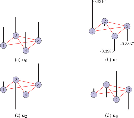
Figure 9.14. Eigenvectors of the graph shown in Figure 9.13(a)

The Eigenvectors for the graph G2 are displayed.

There are four figures labeled alphabetically. All four figures have the following network with four nodes labeled from 1 to 4. The nodes are placed clockwise such that node 1 becomes the topmost node. The followings nodes are connected: 1 and 2, 1 and 3, 1 and 4, 2 and 3, and 2 and 4. Figure a that shows u subscript 0 Eigenvector, vertical lines are drawn from the top of all the nodes with equal magnitudes. Figure b pertains to u subscript 1 and has vertical lines extended up from node 4, and down from nodes 1, 2, and 3. The lengths of the lines correspond to their magnitude values. Figure c corresponds to u subscript 2 with vertical lines extended up from nodes 2, 3, and 4, and down from node 1. The lengths of the lines vary depending on their magnitudes. Figure d corresponds to u subscript 3 with vertical lines extended up from nodes 3 and 4, and down from nodes 1 and 2. The lengths of the lines vary depending on their magnitudes.

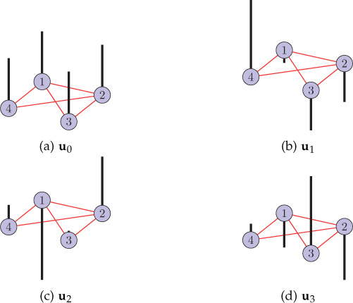
Figure 9.15. Eigenvectors of the graph shown in Figure 9.13(c)

9.6 Generalized Operators for Graph Signals

In classical signal processing, operators such as filtering, convolution, translation, and modulation are frequently utilized in various signal processing tasks. These fundamental operators have also been extended to graph settings [165] through GFT. In this section, we discuss the definitions of these fundamental operators in graph settings. For each of the operators, first its classical definition is presented and subsequently analogy is made to extend the definitions to graph settings.

9.6.1 Filtering

Filtering operation, when viewed in the frequency domain, refers to amplifying some frequencies or attenuating some frequencies to get a new signal. A graph filter can be represented as a matrix, as shown in Figure 9.16, where signal f is the input to the filter H and f_out = Hf is the output of the filter.

Figure 9.16. A graph filter

Spectral Domain Filters

Consider a graph signal f that can be written in terms of the graph harmonics as

(9.6.1) $? = \hat{f} (λ_{0}) ?_{0} + \hat{f} (λ_{1}) ?_{1} + \dots + \hat{f} (λ_{N - 1}) ?_{N - 1},$

where $\hat{f} (λ_{0}), \hat{f} (λ_{1}), \dots, \hat{f} (λ_{N - 1})$ are GFT coefficients. A graph filter modifies (attenuates or amplifies) these GFT coefficients and results an output graph signal f_out.

(9.6.2) $?_{o u t} = \hat{h} (λ_{0}) \hat{f} (λ_{0}) ?_{0} + \hat{h} (λ_{1}) \hat{f} (λ_{1}) ?_{1} + \dots + \hat{h} (λ_{N - 1}) \hat{f} (λ_{N - 1}) ?_{N - 1} .$

Here, $\hat{h} (λ_{0}), \hat{h} (λ_{1}), \dots, \hat{h} (λ_{N - 1})$ are filter coefficients in the frequency domain and are also known as the frequency response of the filter. Thus, each frequency component of the output signal is modified according to the filter coefficient corresponding to that frequency:

(9.6.3) ${\hat{f}}_{o u t} (λ_{ℓ}) = \hat{f} (λ_{ℓ}) \hat{h} (λ_{ℓ}) .$

Equivalently, the above equation can be written in the vertex domain as

(9.6.4) $f_{o u t} (n) = Σ_{ℓ = 0}^{N - 1} \hat{f} (λ_{ℓ}) \hat{h} (λ_{ℓ}) u_{ℓ} (n) .$

In matrix form, the filtering operation provided by Equation (9.6.2) can be expressed as f_out = Hf where

(9.6.5) $? = ? [\begin{matrix} \hat{h} (λ_{0}) & 0 \\ ⋱ \\ 0 & \hat{h} (λ_{N - 1}) \end{matrix}] ?^{T} .$

From Equation (9.6.5), it is clear that the eigenvectors of H are the same as of L. However, the eigenvalues of H change to $\hat{h} (λ_{ℓ})$ . The filter H has N number of parameters: $\hat{h} (λ_{0}), \hat{h} (λ_{1}), \dots, \hat{h} (λ_{N - 1})$ . Using the spectral domain approach to filtering, one can design a filter with an arbitrary frequency response by choosing the N filter parameters accordingly. One important point to note here is that the filter H designed in the spectral domain is not localized; that is, to compute the filtered output at node i (in the spatial domain), one may need the signal values that are not within a fixed number of hops from node i. However, with polynomial filters in the spatial domain, one can design localized filters.

Polynomial Filters in the Spatial Domain

A filter H, given by Equation 9.6.5, is designed in the spectral domain, has N number of parameters, and is not localized in space. However, if we use a filter which is a polynomial in the Laplacian matrix L, localization in space can be achieved; that is to compute the filtered output at node i, we will require the signal values that are within K-hops from node i, where K is the order of the polynomial. Consider a polynomial filter of order K (< N):

(9.6.6) $H = h (L) = Σ_{k = 0}^{K} h_{k} L^{k} = h_{0} I + h_{1} L + \dots + h_{K} L^{K},$

where $h_{0}, h_{1}, \dots, h_{K} \in ℝ$ are called filter taps or filter parameters. Since (L^K)_ij = 0 for $d_{?} (i, j) > K$ (see Problem 16), where $d_{?} (i, j)$ is the hop distance between nodes i and j, the filter H given by Equation 9.6.6 is K-localized at every node.

We can also represent the polynomial filter in the spectral domain. Since the eigendecomposition of K^th power of matrix L is given by L^K = UΛ^KU^T, the filter H given by Equation 9.6.6 can be written as

(9.6.7) $\begin{matrix} H & = Σ_{k = 0}^{K} h_{k} U Λ^{k} U^{T} \\ = U (Σ_{k = 0}^{K} h_{k} Λ^{k}) U^{T} \\ = U h (Λ) U^{T}, \end{matrix}$

where

(9.6.8) $h (?) = [\begin{matrix} h (λ_{0}) & 0 \\ h (λ_{1}) \\ ⋱ \\ 0 & h (λ_{N - 1}) \end{matrix}]$

and

(9.6.9) $h (λ_{ℓ}) = Σ_{k = 0}^{K} h_{k} λ_{ℓ}^{k} = h_{0} + h_{1} λ_{ℓ} + h_{2} λ_{ℓ}^{2} + \dots + h_{K} λ_{ℓ}^{K}$

is a polynomial of order K in eigenvalue λ_ℓ.

9.6.2 Convolution

The classical convolution product of two signals x(t) and h(t) is defined as

(9.6.10) $y (t) = x (t) * h (t) = \int_{ℝ} x (τ) h (t - τ) d τ .$

The above definition of convolution product requires translation of one of the signals. If one tries to extend the above definition to graph signals, it will require translating the graph signal, which is difficult to define in the vertex domain. In such a case, one can utilize frequency domain representation.

The classical convolution theorem states that the convolution product in the time domain is equivalent to multiplication in the frequency domain. Therefore, the convolution product of two signals is equivalent to the inverse Fourier transform of the multiplication of the Fourier transforms of the two signals, that is,

(9.6.11) $y (t) = \int_{ℝ} \hat{x} (ω) \hat{h} (ω) e^{j ω t} d ω .$

In the same way, by utilizing GFT, one can define convolution of two graph signals. Analogous to Equation (9.6.11), the convolution of two graph signals f, g ∈ ℝ^N is defined as

(9.6.12) $(f * g) (n) = Σ_{ℓ = 0}^{N - 1} \hat{f} (λ_{ℓ}) \hat{g} (λ_{ℓ}) u_{ℓ} (n),$

where $\hat{?}$ and $\hat{?}$ are GFTs of f and g, respectively. It is easy to note that the graph convolution also follows classical convolution theorem; that is, the convolution in the vertex domain is equivalent to element-wise multiplication in the graph spectral domain. In matrix form, the convolution product of two graph signal can be written as

(9.6.13) $? = ? * ? = ? (\hat{?} ⊙ \hat{?}),$

where U is the matrix whose columns are the eigenvectors of the graph Laplacian and represents element-wise Hadamard product. As an example, consider two graph signals f and g shown in Figures 9.17(a) and (b). Their convolution product is plotted in Figure 9.17(c), which can be calculated as

Three figures exemplifying graph convolution.

The three figures are labeled alphabetically. All three have the following network with five nodes labeled from 1 to 5. The first four nodes are placed clockwise such that node 1 becomes the leftmost node. The fifth node is positioned to the right of node 4. The followings nodes are connected: 1 and 2, 1 and 3, 2 and 3, 2 and 4, 3 and 4, and 4 and 5. Vertical lines are extended up from all nodes in all three graphs. The lengths of these lines vary according to their magnitude values. Figure a shows the graph signal f with the following written below it: f equals [3, 4, 6, 3, 1] superscript T. The value 3 is written beside the vertical line from node 1. Figure b shows the graph signal g with the following written below it: g equals [4, 2, 4, 2, 2] superscript T. The value 4 is written beside the vertical line from node 1. Figure c shows the Convolution product h equals f star g. The following is written below the graph: h equals [21.92, 23.92, 21.08, 21.72, 17.80] superscript T. The value 21.92 is written beside the vertical line from node 1.

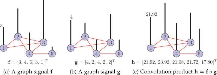
Figure 9.17. Example of graph convolution

$\begin{matrix} ? & = ? (\hat{?} ⊙ \hat{?}) = ? ((?^{T} ?) ⊙ (?^{T} ?)) \\ = ? [\begin{matrix} 7.60 \\ 2.65 \\ - 1.60 \\ - 1.41 \\ - 1.27 \end{matrix}] ⊙ [\begin{matrix} 6.26 \\ 1.39 \\ 0.92 \\ - 1.41 \\ - 0.16 \end{matrix}] = ? [\begin{matrix} 47.60 \\ 3.67 \\ - 1.48 \\ 2.00 \\ 0.21 \end{matrix}] = [\begin{matrix} 21.92 \\ 23.92 \\ 21.08 \\ 21.72 \\ 17.80 \end{matrix}] . \end{matrix}$

The convolution of two graph signals follows the properties of commutativity, distributivity, and associativity (see Exercise Problem 15). The definition graph convolution is utilized in defining graph translation operator.

9.6.3 Translation

In Section 9.1, we saw that translating a graph signal is not as straightforward as translating a 1-D time series. However, the translation operator for graph settings can be defined using the convolution operator defined above.

Classical translation of a signal x(t) by some time τ can be represented using impulse at τ:

(9.6.14) $x (t - τ) = x (t) * δ_{τ} (t) = \int_{ℝ} \hat{x} (ω) \hat{δ_{τ}} (ω) e^{j ω t} d ω = \int_{ℝ} \hat{x} (ω) e^{- j ω τ} e^{j ω t} d ω,$

where δ_τ(t) is an impulse at τ and, using Equation (9.5.1), its Fourier transform is $\hat{δ_{τ}} (ω) = e^{- j ω τ}$ .

Analogously, the generalized translation operator T_i can be defined via generalized convolution with an impulse centered at vertex i:

(9.6.15) $(T_{i} f) (n) = \sqrt{N} (f * δ_{i}) (n) = \sqrt{N} Σ_{ℓ = 0}^{N - 1} \hat{f} (λ_{ℓ}) u_{ℓ}^{*} (i) u_{ℓ} (n),$

where

$δ_{i} (n) = {\begin{matrix} 1 & if n = i \\ 0 & otherwise. \end{matrix}$

In Equation 9.6.15, $\sqrt{N}$ is a normalizing constant to ensure that the translation operator preserves the mean of a graph signal. In matrix form, the translated vector (to node i) can be written as

(9.6.16) $T_{i} ? = \sqrt{N} (? * ?_{i}) = \sqrt{N} ? (\hat{?} ⊙ \hat{?_{i}}) = \sqrt{N} ? (\hat{?} ⊙ {?'}_{i}),$

where ${?'}_{i} = ?^{T} (:, i)$ is the i^th column of U^T and the operator ℓ represents element-wise Hadamard operation.

An example of translation is shown in Figure 9.18. Figure 9.18(a) shows a graph signal f, and Figures 9.18(b) and 9.18(c) show the translated version of f to nodes 1 and 4, respectively. Another example of the translation operation is shown in Figure 9.19. A graph signal on a sensor network is shown in Figure 9.19(a), and the graph signal when translated to the circled node is shown in Figure 9.19(b).

Three figures exemplifying graph translation.

The three figures are labeled alphabetically. All three have the following network with five nodes labeled from 1 to 5. The first four nodes are placed clockwise such that node 1 becomes the leftmost node. The fifth node is positioned to the right of node 4. The followings nodes are connected: 1 and 2, 1 and 3, 2 and 3, 2 and 4, 3 and 4, and 4 and 5. Vertical lines are extended up from all nodes in all three graphs. The lengths of these lines vary according to their magnitude values. Figure a shows the graph signal f with the following written below it: f equals [3, 4, 6, 3, 1] superscript T. The value 3 is written beside the vertical line from node 1. Figure b shows the signal f translated to node 1. The following is written below it: T subscript 1 f equals [2.44, 5.08, 5.08, 3.72, 0.69] superscript T. The value2.44 is written beside the vertical line from node 1. Figure c shows the signal f translated to node 4. The following is written below the graph: T subscript 4 f equals [3.72, 3.56, 3.56, 1.08, 5.08] superscript T. The value 3.72 is written beside the vertical line from node 1.

Figure 9.18. Example of graph translation

The original graph signal and the translated signal are displayed.

The first figure on the left shows the original graph signal. Several nodes are present and are interconnected. The nodes seem to form a U-shape if viewed from the top. The nodes to the right are more densely connected. On the left portion of the graph, several nodes are present in a circle, forming a ring network. All these nodes are connected to a single node at the center of the ring. Vertical lines depending on the magnitude values of the nodes are extended from the top of the nodes. The number of vertical lines and their magnitudes is greater on the right portion of the graph. The second figure on the right shows the signal translated to the circled node. Here the overall network remains the same. The node at the center of the ring of nodes is encircled to look bigger. Now, the number of vertical lines and their magnitudes is greater on the left portion of the graph.

Figure 9.19. Example of translation operator

The translation operator is usually viewed as a kernelized operator acting in the graph spectral domain. The kernel $\hat{f} (.)$ can be used to define the translation of a graph signal f around the graph. Translation of a graph signal to vertex i can be achieved by multiplying the ℓth component of the kernel by $u_{ℓ}^{*} (i)$ , and then taking the IGFT.

The generalized translation operator is utilized to define the WGFT discussed in Section 9.8.

9.6.4 Modulation

Classical modulation of a signal x(t) by a frequency ω is just multiplication of the signal and the complex exponential at frequency ω; that is, the modulated signal is e^jωtx(t). Analogously, in graph settings, the generalized modulation operator M_k is defined as

(9.6.17) $(M_{k} ?) = \sqrt{N} ?_{k} ⊙ ?,$

where the operator ℓ represents element-wise Hadamard operation.

The classical modulation in the time domain is equivalent to translation in the frequency domain, that is, $\hat{M_{ω_{0}} x} (ω) = \hat{x} (ω - ω_{0}), \forall ω \in ℝ$ . On the other hand, because of the irregular nature of the underlying graphs, the generalized modulation defined by Equation 9.6.17 does not represent translation in the graph spectral domain. However, if $\hat{?}$ is localized around zero frequency, then $\hat{M_{k} ?}$ is localized around λ_k. Localization around zero frequency means that most of the non-zero elements are in the vicinity of λ₀ = 0.

9.7 Applications

The ability of the GFT to capture the changes in a graph signal makes it very useful for a number of applications. A few applications are discussed here. First, we present how GFT can be used to explore the structure of various complex network models via performing spectral analysis of node centralities [166]. As a second example, we discuss graph Fourier transform centrality (GFT-C) [167] that utilizes GFT to quantify the importance of a node in a complex network. Finally, we discuss application of GFT in detecting a corrupted sensor in a sensor network just from observing the spectrum of the data.

9.7.1 Spectral Analysis of Node Centralities

Studying the spectral properties of different node centralities allows one to understand the centrality patterns for various networks. The centrality patterns become very informative in the spectral domain. For illustration, different network models such as regular, Erdös-Rényi (ER), small-world, and scale-free networks are considered here. The networks considered here are undirected and unweighted. Different centralities such as degree centrality (DC), closeness centrality (CC), and betweenness centrality (BC) are defined as signals on the networks and subsequently the GFT coefficients (spectrum) of each signal can be observed.

Regular Network

Consider a 4-regular graph generated by taking 100 nodes randomly. The detailed discussion on r-regular graphs can be found in Chapter 2. The DC signal on the graph is plotted in Figure 9.20(a). The vertical bars indicate the signal values at the nodes. DC signal is constant with a value of 4 at all of the nodes. The spectrum of DC signal has only one non-zero frequency component, which is at zero frequency, as shown in Figure 9.20(b).

The centralities as signals on a 4-regular graph and their corresponding spectra are displayed.

There are six figures labeled alphabetically, placed two in a row. The first figure in each row is a network of nodes representing a signal and the second figure is its corresponding spectrum. The signal is a network of numerous nodes that are interconnected. The color of the nodes vary and a gradient scale is marked with values to describe each node. The spectrum is represented by a graph with lambda subscript l values ranging from 0 to 8 in increments of 1 along the horizontal axis, and f circumflex (lambda subscript l) along the vertical axis. Figure a shows a DC signal with all nodes in the network having a darker shade of blue. The gradient scale is marked with the following values from the bottom: 3, 3.5, 4, 4.5, and 5. Figure b shows the Spectrum of DC signal which has the vertical axis marked with values from 0 to 40 in increments of 10. A series of small peaks runs along the horizontal axis from (0.8, 0) to (7.3, 0). In addition to this, a straight vertical line is drawn from (0, 0) to (0, 40). Figure c shows a CC signal with the nodes in the network having both lighter and darker shades of blue. The gradient scale is marked with the following values from the bottom: 0.265, 0.27, 0.275, 0.28, 0.285, 0.29, and 0.295. Figure d shows the Spectrum of CC signal which has the vertical axis marked with values from 0 to 3 in increments of 1. A series of small peaks runs along the horizontal axis from (0.8, 0) to (7.3, 0). In addition to this, a straight vertical line is drawn from (0, 0) to (0, 2.9). Figure e shows a BC signal with the nodes in the network having both darker and lighter shades of blue. The gradient scale is marked with the following values from the bottom: 0.015, 0.02, 0.025, 0.03, and 0.035. Figure f shows the Spectrum of BC signal which has the vertical axis marked with values from 0 to 0.25 in increments of 0.05. A line parallel to the horizontal axis is drawn from the coordinate 0 on the vertical axis. A series of small peaks runs along the horizontal axis from (0.8, 0) to (7.3, 0). The magnitudes of the peaks are a little greater than those in the previous two spectra. In addition to this, a straight vertical line is drawn from (0, 0) to (0, 0.26). The gradient scale in the three figures showing the signals obviously have a lighter shade of blue at the bottom and becomes darker toward the top. All coordinate plots in the spectrum are only approximate.

Figure 9.20. Centralities as signals on a 4-regular graph and their spectra © [2016] IEEE. Reprinted, with permission, from R. Singh, A. Chakraborty, and B. S. Manoj, “On Spectral Analysis of Node Centralities,” in Proceedings of IEEE ANTS 2016, December 2016.

The CC signal on the graph is plotted in Figure 9.20(c) and corresponding spectrum is shown in Figure 9.20(d). The CC signal varies in the range [0.2626, 0.2964]; however, the variations in the CC signal are very small as we go from one node to an adjacent node connected by an edge. CC values of the two adjacent nodes do not differ by a large amount because the closeness of the two adjacent nodes to the rest of the network is almost same. This similarity in closeness is the reason for the absence of significant high-frequency components in the spectrum of CC signal.

The BC signal is plotted in Figure 9.20(e) and has a range in the interval [0.0142, 0.0358]. The BC signal on the regular graph undergoes a very small change as we move from one node to an adjacent node connected by an edge. Observe from Figure 9.20(f) that the spectrum of BC signal also has only a zero frequency component except for a few very small high-frequency components.

ER Network

Consider an ER random graph³ [62] with the probability of 0.06. DC, CC, and BC signals defined on the ER graph are plotted in Figures 9.21(a), (c), and (e), respectively. DC signal values lie in the interval [1, 13] and are randomly distributed over the graph because in an ER graph, an edge exists between every pair of the graph nodes with certain probability (here the probability is 0.06), which contributes to DC signal value at both the corresponding nodes.

The centralities as signals on an ER graph and their corresponding spectra are displayed.

There are six figures labeled alphabetically, placed two in a row. The first figure in each row is a network of nodes representing a signal and the second figure is its corresponding spectrum. The signal is a network of numerous nodes that are interconnected. The color of the nodes vary and a gradient scale is marked with values to describe each node. The spectrum is represented by a graph with lambda subscript l values ranging from 0 to 16 in increments of 2 along the horizontal axis, and f circumflex (lambda subscript l) along the vertical axis. Figure a shows a DC signal with the nodes in the network having both darker and lighter shades of blue. There are more nodes shaded in dark blue. The gradient scale is marked with the following values from the bottom: 2, 4, 6, 8, 10, and 12. Figure b shows the Spectrum of DC signal which has the vertical axis marked with values from 0 to 60 in increments of 20. A line parallel to the horizontal axis is drawn from the coordinate 0 on the vertical axis. A series of small peaks runs along the horizontal axis from (1, 0) to (15, 0). In addition to this, a straight vertical line is drawn from (0, 0) to (0, 60). Figure c shows a CC signal with the nodes in the network having both lighter and darker shades of blue. There are more nodes shaded in the darker shades. The gradient scale is marked with the following values from the bottom: 0.28, 0.3, 0.32, 0.34, 0.36, 0.38, 0.4, and 0.42. Figure d shows the Spectrum of CC signal which has the vertical axis marked with values from 0 to 3 in increments of 1. A line parallel to the horizontal axis is drawn from the coordinate 0 on the vertical axis. A series of small peaks runs along the horizontal axis from (1, 0) to (15, 0). The magnitudes of these peaks are lesser than those in the spectrum in figure b. In addition to this, a straight vertical line is drawn from (0, 0) to (0, 3.7). Figure e shows a BC signal with the nodes in the network having both a darker and lighter shades of blue. There are more nodes shaded in the lighter shades. The gradient scale is marked with the following values from the bottom: 0.01, 0.02, 0.03, 0.04, 0.05, 0.06, and 0.07. Figure f shows the Spectrum of BC signal which has the vertical axis marked with values from 0 to 0.2 in increments of 0.05. A line parallel to the horizontal axis is drawn from the coordinate 0 on the vertical axis. A series of small peaks runs along the horizontal axis from (1, 0) to (15, 0). The magnitudes of the peaks are greater than those in the previous two spectra. In addition to this, a straight vertical line is drawn from (0, 0) to (0, 0.135). The gradient scale in the three figures showing the signals obviously have a lighter shade of blue at the bottom and becomes darker toward the top. All coordinate plots in the spectrum are only approximate.

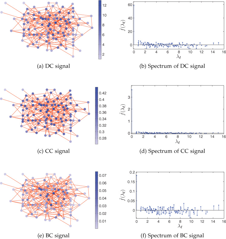
Figure 9.21. Centralities as signals on an ER graph and their spectra © [2016] IEEE. Reprinted, with permission, from R. Singh, A. Chakraborty, and B. S. Manoj, “On Spectral Analysis of Node Centralities,” in Proceedings of IEEE ANTS 2016, December 2016.

The CC signal varies in the interval [0.2612, 0.4381] which is plotted in Figure 9.21(c). It has low value at distant nodes and has high value at the nodes that are central to the network. CC signal variations are small when we move from one node to the adjacent nodes. The BC signal takes a value in the interval [0, 0.0749] and is plotted in Figure 9.21(e). It has more spectral variations as compared to the DC signal.

The spectra of DC, CC, and BC signals are shown in Figures 9.21(b), (d), and (f), respectively. It can be observed from Figure 9.21(b) that the spectrum of DC signal on the ER graph has significant GFT coefficients at low as well as high frequencies. The spectrum of CC signal does not contain high-frequency components, as shown in Figure 9.21(d). The BC signal has stronger frequency components than those of the DC signal, as shown in Figure 9.21(f).

ER Graph with Varying Edge Probability

The above discussion was for an ER graph with a certain fixed edge probability. What about the spectra of DC signal with varying edge probability? Figure 9.22 shows the energy content, except zero frequency, in the spectrum of DC signal with respect to the varying probabilities of edge connection. Observe that the energy increases with increasing probability and becomes maximum for p = 0.5, and then it starts decreasing. For p = 0, the energy is zero because the graph has no edges present in this case; that is, DC signal is a zero vector. Also for p = 1, the energy is zero because the graph becomes regular, where each node is connected to every other nodes in the network. Because the plot is symmetric about p = 0.5, one can also argue that the amount of randomness for probability p is same as for probability (1 − p), and it is maximum for p = 0.5.

A graph with the Edge probability for ER networks plotted against the Energy in DC spectrum.

Figure 9.22. Energy in DC spectrum Versus edge probability for ER networks. Each value is averaged over 1000 experiments. © [2016] IEEE. Reprinted, with permission, from R. Singh, A. Chakraborty, and B. S. Manoj, “On Spectral Analysis of Node Centralities,” in Proceedings of IEEE ANTS 2016, December 2016.

Small-World Network

Consider a small-world network⁴ generated by adding a few LLs (5%–8% of the total nodes) in a regular rectangular grid network. DC, CC, and BC signals on a 100 node network are plotted in Figures 9.23(a), (c), and (e), respectively. DC signal lies in the interval [2, 6] as shown in Figure 9.23(a). The CC signal varies in the range of [0.1343, 0.2878], which is shown in Figure 9.23(c). The CC signal has minimal variation as one moves from one node to the other connected by an edge because closeness of any two adjacent nodes, to the rest of the network, does not have a large difference. The CC signal has peaks at the nodes, which are the extremes of LLs; however, the signal value decreases slowly as we move away from these nodes. The range of BC signal is in the interval [0, 0.3148] as shown in Figure 9.23(e). The LLs in a small-world network are present in most of the shortest paths between any two distant nodes; therefore, the nodes corresponding to LLs have high BC value.

Spectra of DC, CC, and BC signals are plotted in Figures 9.23(b), (d), and (f), respectively. The spectrum of DC signal has small values of GFT coefficients at low frequencies, as shown in Figure 9.23(b). High-frequency components are very small in the spectrum. The spectrum of CC signal on the small-world graph is also localized around zero frequency; that is, it has only mild low frequency components (see Figure 9.23(d)). However, one can observe from Figure 9.23(f) that the BC signal on the small-world graph contains some strong low-frequency as well as high-frequency components. As we move from the nodes which have high BC value to any other adjacent node except the node connected via LLs, the BC value changes significantly. These changes in BC value results in the presence of significant high-frequency components in the spectrum of BC signal. Comparing Figures 9.23(f) and 9.23(b), it can be observed that there are relatively stronger high-frequency components present in the spectrum of BC signal than in that of the DC signal, because the BC value at the nodes corresponding to LLs has relatively larger value than the DC value at the corresponding nodes.

The centralities as signals on a small-world network and their corresponding spectra are displayed.

There are six figures labeled alphabetically, placed two in a row. The first figure in each row is a network of nodes representing a signal and the second figure is its corresponding spectrum. The signal is a 10 cross 10 grid network with nodes at the vertices of the grid. The nodes are obviously connected to those around it. Some nodes are randomly connected also. The color of the nodes vary and a gradient scale is marked with values to describe each node. The spectrum is represented by a graph with lambda subscript l values ranging from 0 to 9 in increments of 1 along the horizontal axis, and f circumflex (lambda subscript l) along the vertical axis. Figure a shows a DC signal with the nodes in the network having both darker and lighter shades of blue. There are more nodes shaded in dark blue. The nodes at the center of the grid appear darker and the shade lightens as we go away from the center. The gradient scale is marked with the following values from the bottom: 2, 3, 4, 5, and 6. Figure b shows the Spectrum of DC signal which has the vertical axis marked with values from 0 to 40 in increments of 10. A line parallel to the horizontal axis is drawn from the coordinate 0 on the vertical axis. A series of small peaks runs along the horizontal axis from (0.1, 0) to (8.7, 0). In addition to this, a straight vertical line is drawn from (0, 0) to (0, 48). Figure c shows a CC signal with the nodes in the network having both lighter and darker shades of blue. There is almost an equal number of nodes in both shades. The nodes at the center of the grid appear darker and the shade lightens as we go away from the center. The gradient scale is marked with the following values from the bottom: 0.14, 0.16, 0.18, 0.2, 0.22, 0.24, 0.26, and 0.28. Figure d shows the Spectrum of CC signal which has the vertical axis marked with values from 0 to 2 in increments of 0.5. A line parallel to the horizontal axis is drawn from the coordinate 0 on the vertical axis. A series of small peaks runs along the horizontal axis from (0.1, 0) to (8.7, 0). The magnitudes of these peaks are lesser than those in the spectrum in figure b. In addition to this, a straight vertical line is drawn from (0, 0) to (0, 2). Figure e shows a BC signal with the nodes in the network having both a darker and lighter shades of blue. There are more nodes shaded in the lighter shades and only countable nodes in the darker shades scattered in the network. The gradient scale is marked with the following values from the bottom: 0.05, 0.1, 0.15, 0.2, 0.25, and 0.3. Figure f shows the Spectrum of BC signal which has the vertical axis marked with values from 0 to 0.4 in increments of 0.1. A line parallel to the horizontal axis is drawn from the coordinate 0 on the vertical axis. A series of small peaks runs along the horizontal axis from (0.1, 0) to (8.7, 0). The magnitudes of the peaks are greater than those in the previous two spectra. In addition to this, a straight vertical line is drawn from (0, 0) to (0, 0.42). The gradient scale in the three figures showing the signals obviously have a lighter shade of blue at the bottom and becomes darker toward the top. All coordinate plots in the spectrum are only approximate.

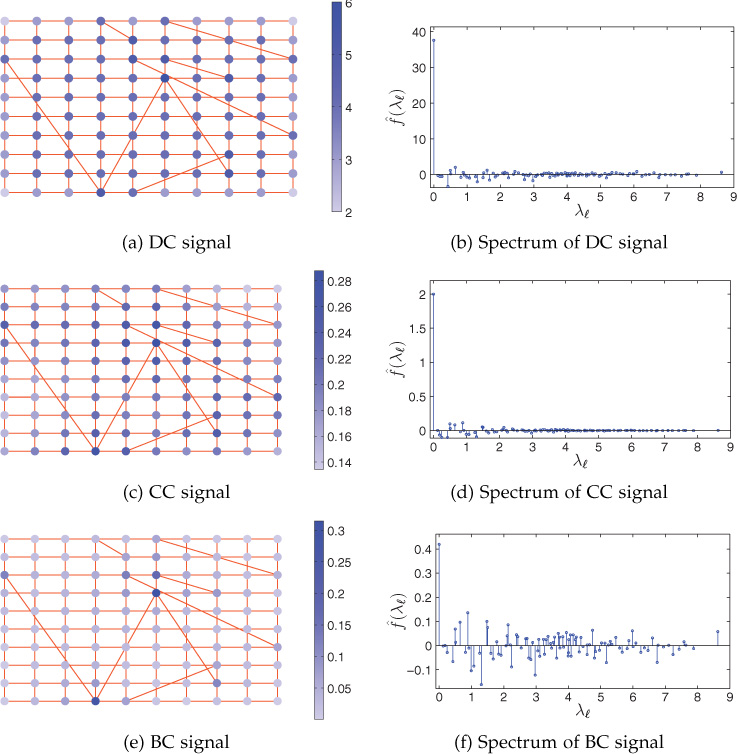
Figure 9.23. Centralities as signals on a small-world network and their spectra © [2016] IEEE. Reprinted, with permission, from R. Singh, A. Chakraborty, and B. S. Manoj, “On Spectral Analysis of Node Centralities,” in Proceedings of IEEE ANTS 2016, December 2016.

Watts-Strogatz Network Model with Varying Rewiring Probability

Consider a small-word network generated by the Watts-Strogatz model [6] and then compute the energy of the DC signal lying in non-zero frequency components of the spectrum. Repeat the experiment with varying rewiring probability and compute the corresponding energies, the plot of which is shown in Figure 9.24. Observe the increase in energy with the rewiring probability, which shows the increase in randomness of the network with increasing rewiring probability.

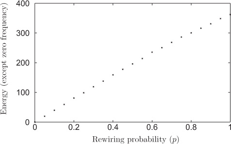
A graph with the Rewiring probability for Watts-Strogatz small-world networks plotted against the Energy in DC spectrum.

Figure 9.24. Energy in DC spectrum versus rewiring probability for Watts-Strogatz small-world networks. Each value is averaged over 1000 experiments. © [2016] IEEE. Reprinted, with permission, from R. Singh, A. Chakraborty, and B. S. Manoj, “On Spectral Analysis of Node Centralities,” in Proceedings of IEEE ANTS 2016, December 2016.

Scale-Free Network

Consider the Barabási-Albert model [39] for the creation of a scale-free network⁵ with γ = 3. DC, CC, and BC signals on a 100-node scale-free network are shown in Figures 9.25(a), (c), and (e), respectively. The DC signal on the network varies in the interval [1, 14], as shown in Figure 9.25(a). It can be observed that only a few nodes (known as hub nodes) in the graph have large DC values, and a large number of nodes have small DC values. As we move from the hub node to any other adjacent node, the DC signal value changes drastically. The range of the BC signal is [0, 0.6778], as plotted in Figure 9.25(e). The value of the BC signal is also very large at the hub nodes, and it undergoes large variations when we move to other adjacent nodes. The large value of BC at hub nodes is because the hub nodes are present in most of the shortest paths in the graph. The CC signal varies in the interval [0.1292, 0.3438], which is plotted in Figure 9.25(c). It has small values at distant nodes and large values at the nodes that are more central to the network. Although the CC signal has peaks at hub nodes too, it does not change rapidly as we move from a hub node to any other adjacent node, because the closeness of the node to the entire graph does not change significantly.

There are six figures labeled alphabetically, placed two in a row. The first figure in each row is a network of nodes representing a signal and the second figure, its corresponding spectrum. The signal is depicted as a network of nodes. The network appears to have about nine clusters, with each cluster having a central node that branches out to connect multiple nodes. The center nodes of two clusters are connected with or without an intermediate node to being the network together. The color of the nodes vary and a gradient scale is marked with values to describe each node. The spectrum is represented by a graph with lambda subscript l values ranging from 0 to 16 in increments of 2 along the horizontal axis, and f circumflex (lambda subscript l) along the vertical axis. Figure a shows a DC signal with the nodes in the network having both darker and lighter shades of blue. The center nodes are shaded in dark blue. The gradient scale is marked with the following values from the bottom: 2, 4, 6, 8, 10, 12, and 14. Figure b shows the Spectrum of DC signal which has the vertical axis marked with values from -10 to 20 in increments of 10. A line parallel to the horizontal axis is drawn from the coordinate 0 on the vertical axis. Vertical lines of different magnitudes are drawn along this line from (0, 0) to (15, 0). The vertical lines are either extended above or below the horizontal line at the 0th coordinate. Figure c shows a CC signal with the nodes in the network having both lighter and darker shades of blue. There is almost an equal number of nodes in both shades. The center nodes are a dark blue while the shade lightens as the outermost node of each cluster is reached. The gradient scale is marked with the following values from the bottom: 0.15, 0.2, 0.25, and 0.3. Figure d shows the Spectrum of CC signal which has the vertical axis marked with values from 0 to 2 in increments of 0.5. A line parallel to the horizontal axis is drawn from the coordinate 0 on the vertical axis. Vertical lines of different magnitudes are drawn along this line from (0, 0) to (15, 0). The vertical lines are either extended above or below the horizontal line at the 0th coordinate. The magnitudes of these peaks are lesser than those in the spectrum in figure b, except the first line from (0, 0) to (0, 2.2). Figure e shows a BC signal with the nodes in the network having both a darker and lighter shades of blue. There are more nodes shaded in the lighter shades and only the center nodes are in the darker shades. The gradient scale is marked with the following values from the bottom: 0, 0.1, 0.2, 0.3, 0.4, 0.5, and 0.6. Figure f shows the Spectrum of BC signal which has the vertical axis marked with values from -0.4 to 0.8 in increments of 0.2. A line parallel to the horizontal axis is drawn from the coordinate 0 on the vertical axis. Vertical lines of different magnitudes are drawn along this line from (0, 0) to (15, 0). The vertical lines are either extended above or below the horizontal line at the 0th coordinate. The magnitudes of the peaks are greater than those in the previous two spectra. The gradient scale in the three figures showing the signals obviously have a lighter shade of blue at the bottom and becomes darker toward the top. All coordinate plots in the spectrum are only approximate.

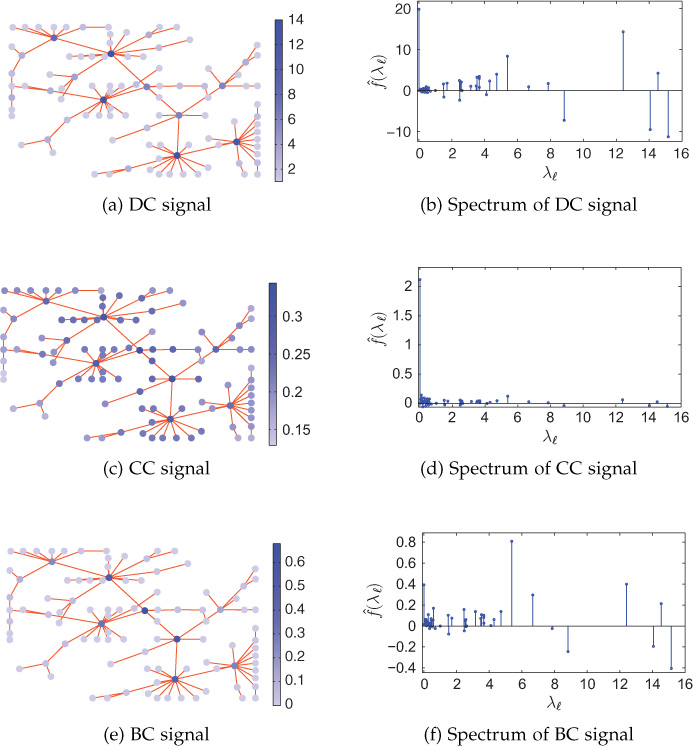
Figure 9.25. Centralities as signals on a scale-free network and their spectra © [2016] IEEE. Reprinted, with permission, from R. Singh, A. Chakraborty, and B. S. Manoj, “On Spectral Analysis of Node Centralities,” in Proceedings of IEEE ANTS 2016, December 2016.

The spectra of the DC, CC, and BC signals on the scale-free network are plotted in Figures 9.25(b), (d), and (f), respectively. One can observe from Figure 9.25(b) that the DC signal on scale-free graph has very strong high-frequency components, as there is a drastic change in signal value from hub node to neighbor nodes. The BC signal also contains very strong high-frequency components, as shown in Figure 9.25(f). However, the CC signal has very small high-frequency components, as shown in Figure 9.25(d), because of minimal variation of the signal as one moves from one node to another. Compared to all other graphs, the spectra of DC and BC signals on scale-free graphs have much stronger high-frequency components, which shows the presence of hub nodes in scale-free networks.

Network Classification from the Spectra of Centrality Signals

We have seen the spectral patterns of centrality measures on various networks. Given the spectra of node centralities as signals on a network, the type of the network can be identified. If the spectrum of DC signal on a network has only non-zero GFT coefficient at zero frequency, then the underlying network is an r-regular network with $r = \frac{\hat{f} (λ_{0})}{\sqrt{N}}$ where $\hat{?}$ is GFT of DC signal f and N is the total number of nodes in the network.

Presence of stronger high-frequency components than low-frequency components in the spectrum of DC or BC signal on the network indicates that the underlying network is scale-free. The identification of scale-free network and regular network from the spectrum of DC signal can be done accurately.

If the spectrum of DC signal has significant frequency components over all the frequencies, then the underlying network can be a small-world or an ER network. Picking one of these two networks accurately is difficult. However, from analysis done previously, it can be argued that as the small-worldness of the network increases, more and more high-frequency components exist in the spectrum of DC. Also, even for a random network with a high degree of randomness (edge probability of 0.5 in ER model), high-frequency content in the spectrum of the network is not as strong as in case of scale-free networks.

9.7.2 Graph Fourier Transform Centrality

GFT-C is a spectral approach for assessing the importance of each node in a complex network [167]. GFT-C uses GFT coefficients of an importance signal corresponding to the reference node. This method relies on the global smoothness (or variations) of the carefully defined importance signal corresponding to a reference node. The importance signal for a reference node is the indicator of how remaining nodes in a network are seeing the reference node individually. The importance signal is defined in such a way that the importance information is captured in the global smoothness (or variations) of the signal. Further, GFT coefficients of the importance signal are used to obtain the global view of the reference node.

GFT-C of i^th node is the weighted sum of the GFT coefficients of importance signal corresponding to node i. The importance signal for a reference node i is a graph signal which gives the individual view of the rest of the nodes about reference node i in terms of the minimum cost to reach i. Smoothness of this importance signal is the key in quantifying the importance of the corresponding node. GFT is used to capture the variations in the importance signal globally, which in turn is utilized to define GFT-C. Thus, GFT-C utilizes not only the local properties, but also the global properties of a network topology.

The Importance Signal

The importance signal describes the relation of a reference node to the rest of the nodes individually. It is characterized by the inverse of the cost to reach from an individual node to the reference node. The higher the cost to reach the reference node, the lower is the importance of the reference node, and vice versa.

Let the importance signal corresponding to reference node n on a connected weighted network be f_n = [ f_n(1) f_n(2) ... f_n(N)]^T, where f_n(i) is the inverse of the sum of weights in the shortest path from node i to node n. Normalize the signal such that the sum of signal values, except at the reference node, is unity, that is ∑_i≠_n f_n(i) = 1. Also, consider the signal value at the reference node as unity (f_n(n) = 1).

Figure 9.26 shows a sample weighted graph having 10 nodes. The importance signal along with the intermediate parameters corresponding to node 1 of Figure 9.26 are listed in Table 9.3. It is evident that as the cost to reach the reference node decreases, the value of the importance signal increases.

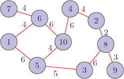
An example weighted graph with 10 nodes.

Figure 9.26. An example weighted graph

Table 9.3. Importance signal for node 1 of graph shown in Figure 9.26 as reference. Reprinted from Elsevier Physica A: Statistical Mechanics and Its Applications, Vol. 487, R. Singh, A. Chakraborty, and B. S. Manoj, GFT centrality: A new node importance measure for complex networks, Pages 185–195, December 2017, Copyright (2017), with permission from Elsevier.

Node	Shortest Path	Cost	(Cost)⁻1	Importance Signal
1	-	0	-	1
2	2-8-3-5-1	19	1/19	0.0550
3	3-5-1	11	1/11	0.0950
4	4-10-6-1	16	1/16	0.0653
5	5-1	6	1/6	0.1742
6	6-1	4	1/4	0.2614
7	7-6-1	8	1/8	0.1307
8	8-3-5-1	17	1/17	0.0615
9	9-8-3-5-1	20	1/20	0.0523
10	10-5-1	10	1/10	0.1045

The variations in the importance signal defined above are utilized to score the importance of a reference node. Also note that for a reference node with high global importance, the importance signal values in the neighborhood of the node will be smaller as compared to a reference node with low global importance but having the same value of DC. The reason behind this is that the sum of the importance signal values, except at the reference node, is unity and the importance signal value is inversely related to the cost to reach the reference node. Therefore, for a reference node with high global importance, from which the rest of the nodes are not very distant, the distribution of importance signal values is such that the neighboring nodes of the reference node receive small values. On the other hand, when the reference node is of low global importance, the neighboring nodes receive high importance signal values because there will be some nodes in the network that are very far from the reference node. These variations in the importance signal, which are captured using GFT, are utilized to quantify the importance of the reference node.

Graph Fourier Transform Centrality

GFT-C measures the importance of a reference node for rest of the network nodes collectively. To define GFT-C for a reference node, GFT coefficients of importance signal are used.

GFT of importance signal is known as importance spectrum. In Figure 9.27, the importance spectra for a few nodes in the network shown in Figure 9.26 are presented. The importance spectra corresponding to node 7 has nominal high-frequency components (Figure 9.27(a)), whereas large high-frequency components are present in the importance spectra of node 10 (Figure 9.27(b)). The importance spectra corresponding to node 3 has moderate GFT coefficients corresponding to high-frequencies (Figure 9.27(c)). From these observations, it can be argued that the importance information is encoded in the high-frequency components of the importance spectrum. The observations from Figure 9.27 are quite intuitive and follow from the fact that if a node is central to the network, then the importance signal is non-smooth, that is, variations in the importance signal are high. Based on these observations, the importance of a reference node can be quantified using the importance spectrum.

Three illustrations of the Importance spectrum for a weighted graph with 10 nodes.

The illustrations are labeled alphabetically, and pertain to the Importance spectra of nodes 7, 10, and 3, respectively. The horizontal axis is marked with lambda subscript l values from 0 to 6 in unit increments. The vertical axis is labeled with f circumflex (lambda subscript l) values. A line is drawn parallel to the horizontal axis from the point (0, 0). Vertical lines are drawn either above or below this line for every half-unit along the horizontal line. The magnitude of the lines vary. Figure a shows the importance spectrum of node 7. The vertical axis is marked from -0.4 to 0.6 in increments of 0.2. The vertical lines are drawn with the following magnitudes that are graded against the vertical axis: 0.6, 0.6, -0.4, -0.3, -0.2, 0, 0.1, -0.05, 0.5, and 0.5. Figure b corresponds to the importance spectrum of node 10. The vertical axis is marked from -0.5 to 0.5 in increments of 0.5. The vertical lines are drawn with the following magnitudes that are graded against the vertical axis: 0.7, 0.2, 0.3, 0.05, 0.25, -0.45, -0.4, -0.3, 0.2, and 0.4. Figure c corresponds to the importance spectrum of node 3. The vertical axis is marked from -0.5 to 0.5 in increments of 0.5. The vertical lines are drawn with the following magnitudes that are graded against the vertical axis: 0.7, -0.2, 0.05, 0.4, -0.6, -0.2, 0.1, 0.2, -0.25, and 0.15. The values mentioned are approximate.

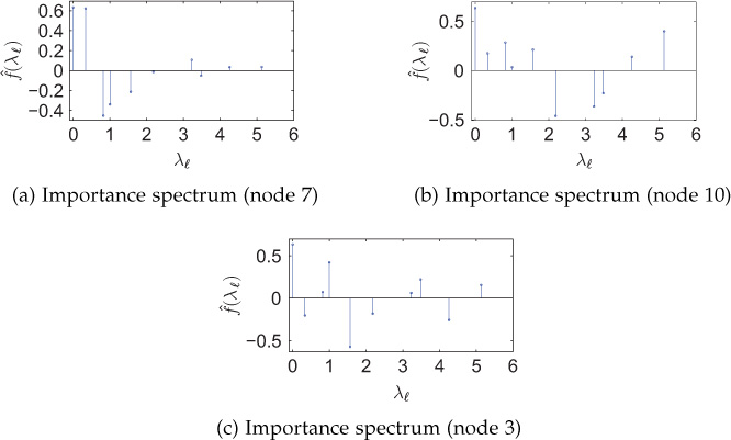
Figure 9.27. Importance spectra for the network topology shown in Figure 9.26. Reprinted from Elsevier Physica A: Statistical Mechanics and Its Applications, Vol. 487, R. Singh, A. Chakraborty, and B. S. Manoj, GFT centrality: A new node importance measure for complex networks, Pages 185–195, December 2017, Copyright (2017), with permission from Elsevier.

Let the GFT of importance signal corresponding to reference node n be ${\hat{?}}_{n} = [{\hat{f}}_{n} (λ_{0}) {\hat{f}}_{n} (λ_{1}) \dots {\hat{f}}_{n} (λ_{N - 1})]^{T}$ , which can be calculated as

(9.7.1) ${\hat{f}}_{n} (λ_{ℓ}) = Σ_{i = 1}^{N} f_{n} (i) u_{ℓ}^{*} (i),$

where f_n(i) is the importance of the reference node n with respect to node i and u_ℓ is the eigenvector of the graph Laplacian at the node corresponding to the eigenvalue λ_ℓ. Let the GFT-C of node n be I_n, then

(9.7.2) $I_{n} = Σ_{ℓ = 0}^{N - 1} w (λ_{ℓ}) | {\hat{f}}_{n} (λ_{ℓ}) |,$

where w(λ_ℓ) is the weight assigned to the GFT coefficient corresponding to frequency λ_ℓ. The choice of weights is made by a function which increases exponentially with the frequency (eigenvalues of L), that is w(λ_ℓ) = e^(kλ_ℓ) − 1, where k > 0. Choosing such weights ensures that (i) larger weights are assigned to high-frequency components of the importance spectrum and smaller weights for the frequency components corresponding to lower frequencies and (ii) zero weight is assigned to zero frequency component. It is found experimentally that k = 0.1 shows good results. Table 9.4 shows GFT-C of the nodes, as found by using Equation (9.7.2), in the network shown in Figure 9.26. It can be observed that node 10 has the highest score and node 9 has the lowest score.

Table 9.4. GFT-C for nodes in the network shown in Figure 9.26. Reprinted from Elsevier Physica A: Statistical Mechanics and Its Applications, Vol. 487, R. Singh, A. Chakraborty, and B. S. Manoj, GFT centrality: A new node importance measure for complex networks, Pages 185–195, December 2017, Copyright (2017), with permission from Elsevier.

Node	1	2	3	4	5	6	7	8	9	10
GFT-C	0.099	0.093	0.103	0.106	0.121	0.135	0.044	0.118	0.040	0.141

GFT-C Behavior on a String Topology Network

First, consider a network with string topology (path graph) which is shown in Figure 9.28. Various centrality scores are listed in Table 9.5, from which we observe that GFT-C scores for end nodes are low, and as we go toward middle nodes, the value of GFT-C increases. It shows superiority over DC as all the nodes except two end nodes have same DC scores of 2, which is not desirable. BC, CC, and eigenvector centrality (EC) also follow the same pattern as GFT-C.

Figure 9.28. A path graph

Table 9.5. Various centrality scores for nodes in the network shown in Figure 9.28. Reprinted from Elsevier Physica A: Statistical Mechanics and Its Applications, Vol. 487, R. Singh, A. Chakraborty, and B. S. Manoj, GFT centrality: A new node importance measure for complex networks, Pages 185–195, December 2017, Copyright (2017), with permission from Elsevier.

Node	A	B	C	D	E	F
DC	1	2	2	2	2	1
BC	0	0.4	0.6	0.6	0.4	0
CC	0.333	0.454	0.555	0.555	0.454	0.333
EC	0.099	0.178	0.223	0.223	0.178	0.099
GFT-C	0.0936	0.1979	0.2085	0.2085	0.1979	0.0936

GFT-C Behavior on an Unweighted Arbitrary Network

Consider an unweighted graph which contains more than just one neighborhood of nodes with high influence, as in Figure 9.29. Since CC and BC measure global importance, they find nodes t and s as the most important nodes, which can be found from Figures 9.29(a) and 9.29(b). On the other hand, though the nodes p, q, and u are influential in their respective neighborhoods, their CC and BC scores are small, implying the inability of CC and BC to capture local influence. Figure 9.29(c) shows the EC scores of nodes in the network. We observe that EC scores are high in the neighborhood of nodes p and q, while the rest of the network nodes receive very small EC scores. This is due to the nature of EC, which tends to focus on a set of influential nodes that are all within the same region (or community) of a graph and particularly focuses on the largest community [168]. DC scores of nodes are shown in Figure 9.29(d), from which we observe that nodes t and υ receive the same DC score of 3. However, this may not be desirable, as node t is more influential than node υ globally. The difference between DC and GFT-C can also be observed in other nodes of the network with the same DC scores. In comparison to DC, CC, BC, and EC, GFT-C takes local as well as global properties of the network into account and results in high importance for the nodes p, q, t, and u, as can be found in Figure 9.29(e).

Five illustrations of the different centrality measures for an unweighted graph.

The five illustrations are labeled alphabetically and pertain to CC, BC, EC, DC, and GFT-C. The network comprises of 20 nodes of which 7 are labeled from p to v. Node p is connected to q below it, r to its left, and two other nodes on its right. Node q is connected to two nodes, one on either side of it and node s to its bottom-left. Node s is connected to node t further to its left. Node t is connected to one node on its left which is connected to a node forming the bottom vertex of a triangle. The other two vertices of this triangle also have nodes. Node t is then connected to a node below it, which is connected to a node on its bottom-left and node u on its bottom-right. These two nodes are connected to a single node below them. Node u is further connected to node v that forms the vertex of a triangle. The other two vertices of this triangle also have nodes. Each of the nodes is shaded in different shades of brown, and the gradient scale is present to the right in every figure. Figure a pertains to CC and the gradient scale is marked with the following values from the bottom: 0.2, 0.25, 0.3, and 0.35. Figure b pertains to BC and the gradient scale is marked with the following values from the bottom: 0, 0.1, 0.2, 0.3, 0.4, 0.5, and 0.6. Figure c pertains to EC and the gradient scale is marked with the following values from the bottom: 0.05, 0.1, and 0.15. Figure d pertains to DC and the gradient scale is marked with values from 1 to 6 in unit increments, bottom-up. Figure a pertains to CC and the gradient scale is marked with values from 0.02 to 0.07 in increments of 0.02 from the bottom. The gradient scale obviously has a lighter shade of brown at the bottom and becomes darker toward the top. The shades of the nodes vary from figure to figure.

Figure 9.29. Various centrality measures for an unweighted graph. Reprinted from Elsevier Physica A: Statistical Mechanics and Its Applications, Vol. 487, R. Singh, A. Chakraborty, and B. S. Manoj, GFT centrality: A new node importance measure for complex networks, Pages 185–195, December 2017, Copyright (2017), with permission from Elsevier.

9.7.3 Malfunction Detection in Sensor Networks

Another example application of GFT and graph filtering can be found in sensor networks where any malfunctions of sensors can be detected from the data generated by the sensors in the network. Consider a temperature sensor network in which nodes represent the weather stations collecting the temperature. Assume that the cities (weather stations) are located close to each other and, therefore, have almost similar temperatures. The temperature measurements can be treated as a graph signal, and observing the GFT coefficients of this graph signal, any sensor malfunction can be detected. If one observes the spectrum of the temperature snapshot (temperature graph signal), most of the energy will be concentrated in the low frequencies given that all the sensor measurements are correct. However, the measurements from a defected sensor may differ from the adjacent sensors drastically, and this drastic change will appear as significant high-frequency components in the spectrum of the temperature snapshot. Thus, if the spectrum of the temperature graph signal constitutes significant high-frequency components, one can conclude that there is at least one sensor with corrupted measurement. Note that, however, the locations of the corrupted sensors by observing the spectrum cannot be found.

9.8 Windowed Graph Fourier Transform

The windowed Fourier transform (WFT), or short-time Fourier transform, is another important tool for time-frequency analysis in classical signal processing. It is particularly useful in extracting information from signals with frequencies that are localized in time. For example, consider a continuous-time signal x(t), shown in Figure 9.30, which contains sinusoids of three different frequencies: 3 Hz from 0 to 1 second, 8 Hz from 1 to 2 seconds, and 4 Hz from 2 to 3 seconds. The frequency information in this signal is local. If we use Fourier transform of this signal, we will not get any information of this time localization of frequencies. Such signals appear frequently in applications such as audio and speech processing, vibration analysis, and radar detection. Localization in time is achieved using an appropriate window function centered around a location of interest. Now consider a rectangular window g(t) of duration 1 second, as shown in Figure 9.30(b). The figure also shows translated versions of window g(t). Multiplying signal x(t) with window g(t), results in a part of signal x(t) from 0 to 1 second, and then Fourier transform of this windowed signal can be used to extract the frequency information in this time duration. Similarly, signal x(t) is multiplied with the translated versions of the window g(t), and then Fourier transform is used to get time-localized frequency information in the signal. Thus, short-time Fourier transform provides a means for time-frequency representation of a signal, through which both time and frequency information can be extracted.

The first figure is labeled Continuous-time signal with 3 sinusoids of different frequencies. The signal is depicted on a graph with the horizontal and vertical axes marked with time t in seconds and x(t), respectively. Time t is marked from 0 to 3 in increments of 0.5, while x(t) is marked from -1 to 1 in increments of 0.2. The height of each cycle of the signal ranges constantly from -1 to 1 along the vertical axis. The first cycle ranges for about 50 seconds, beginning at (0, 1) and ends at (0.75, 0). The next eight cycles are of a smaller time gap each ranging for only about 25 seconds. The final four signals again last for about 75 seconds. The time values are only approximate. The second figure is labeled Rectangular windows at different locations. Three windows are present, one below the other. All three are marked with time t in seconds along the horizontal axis with values ranging from 0 to 3 in increments of 0.5. The vertical axis is marked with a function of t namely g(t), g(t-1), and g(t-2) form the top to bottom, respectively. The values along the vertical axis are 0, 0.5, and 1, in all three windows. In the first window showing the signal at g(t), the signal begins at (0, 1), proceeds as a straight line up to (1, 1), and falls here to the point (1, 0). It then continues as a straight line up to (3, 0). In the second window showing the signal at g(t-1), the signal begins at (0, 0), proceeds as a straight line up to (1, 0), and rises here to the point (1, 1). It then continues as a straight line up to (2, 1), where it falls to (2, 0), and proceeds as a straight line again up to (3, 0). In the third window showing the signal at g(t-2), the signal begins at (0, 0), proceeds as a straight line up to (2, 0), and rises here to the point (2, 1). It then continues as a straight line up to (3, 1).

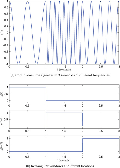
Figure 9.30. A continuous-time signal with 3 sinusoids of different frequencies and window signals

Windowed Fourier analysis has been generalized to the graph settings, and analogously, WGFT has been defined. As mentioned in Section 9.5, GFT is a global transform—it does not convey any information regarding where in a graph the frequency contents are present. Through WGFT, one can find the local information of frequency content in a graph signal.

Classical windowed Fourier transform is defined through two operators: translation and modulation. For a signal x(t) and $t_{0} \in ℝ$ , the translation operator T_t₀ is defined as

(9.8.1) $(T_{t_{0}} x) (t) = x (t - t_{0}),$

The translation operator is used to move a window along the time axis. Moreover, for any $ω \in ℝ$ , the modulation operator M_ω is defined as

(9.8.2) $(M_{ω} x) (t) = e^{j ω t} x (t) .$

Now let g(t) be a window with ||g||₂ = 1. Then a windowed Fourier atom is given by

(9.8.3) $g_{t_{0}, ω} (t) = (M_{ω} T_{t_{0}} g) (t) = g (t - t_{0}) e^{j ω t} .$

WFT of a classical signal x(t) is defined as

(9.8.4) $S x (t_{0}, ω) = ⟨ x, g_{t_{0}, ω} ⟩ = \int_{\infty}^{\infty} x (t) [g (t - t_{0})]^{*} e^{- j ω t} d t .$

Alternatively, WFT of a signal x(t) can also be interpreted as the Fourier transform of the windowed signal. The windowed signal localizes the signal to a specific time. Thus, WFT of a signal is an expansion in terms of two variables: frequency and time-shift.

To define WGFT, generalized translation and modulation operators defined in the Section 9.6 are used. The generalized translation operator is used to move a window around the graph, and then it is multiplied with a graph signal to localize the signal to a specific region of the graph. Analogous to Equation 9.8.3, for a window $? \in ℝ^{N}$ , windowed graph Fourier atom can be defined as

(9.8.5) $\begin{matrix} ?_{i, k} & = M_{k} T_{i} ? \\ = M_{k} (\sqrt{N} ? (\hat{?} ⊙ {?'}_{i})) \\ = \sqrt{N} ?_{k} ⊙ (\sqrt{N} ? (\hat{?} ⊙ {?'}_{i})) \\ = N ?_{k} ⊙ (? (\hat{?} ⊙ {?'}_{i})) . \end{matrix}$

Subsequently, the WGFT coefficient, corresponding to frequency λ_k and centered at node i, of a graph signal $? \in ℝ^{N}$ is defined as

(9.8.6) $S_{i, k} ? = ⟨ ?, ?_{i, k} ⟩ .$

Using WGFT coefficients, one can identify the frequency contents of a graph signal at various vertex locations of the graph. As opposed to the GFT (which is a global transform), the WGFT provides us means to analyze a graph signal locally in the graph.

9.8.1 Example of WGFT

Consider a random sensor network with 48 nodes, as shown in Figure 9.31(a). The network is generated by randomly placing 48 nodes in [0, 1] × [0, 1] plane, and the edge weights are assigned with a threshold Gaussian kernel weighting function based on the Euclidean distance between nodes:

The illustrations of a sensor network, heat kernel, graph Fourier atom, and signal are displayed.

There are four figures labeled alphabetically and placed, two in a row. The same network is used in the figures a, c, and d. Several nodes are present in the network and are interconnected. The nodes seem to form a U-shape if viewed from the top. The nodes to the right are more densely connected. On the left portion of the graph, several nodes are present in a circle, forming a ring network. All these nodes are connected to a single node at the center of the ring. Figure a shows this Sensor network wherein the node at the center of the ring is encircled to look bigger. Figure b is labeled the Heat kernel. It has a horizontal axis marked with lambda subscript l values ranging from 0 to 10 in increments of 2. The vertical axis is graded with g circumflex (lambda subscript l) values from 0 to 1.5 in increments of 0.5. Vertical lines with their peaks marked and varying magnitudes are drawn from the horizontal axis above or below it. Only the first four line are predominant: (0, 0) to (0, 1.49), (0.1, 0) to (0.1, 1.1), (0.3, 0) to (0.3, 0.5), and (0.5, 0) to (0.5, 0.25). The lines continue to be marked minutely up to the point (11, 0). Figure c shows the Graph Fourier atom g subscript (34, 15). Vertical lines depending on the magnitude values of the nodes are extended from the top of the nodes. These lines are drawn only from a few nodes connected in the ring on the left of the network. Figure d shows the Signal f, wherein vertical lines are extended from the top or bottom of each node depending on their magnitude values.

Figure 9.31. Windowed graph Fourier transform example

(9.8.7) $w_{i j} = {\begin{matrix} e x p (- \frac{[d (i, j)]^{2}}{2 σ_{1}^{2}}) & if d (i, j) \leq σ_{2} \\ 0 & otherwise, \end{matrix}$

where d(i, j) is the Euclidean distance between nodes i and j, σ₁ = 0.074, and σ₂ = 0.075. Using a heat kernel shown in Figure 9.31(b), graph Fourier atoms corresponding to a graph frequency can be computed. A windowed graph Fourier atom g34,15 corresponding to frequency λ₁₅ = 4.94 and centered at vertex 34 is shown in Figure 9.31(c). The corresponding WGFT coefficient of the graph signal shown in Figure 9.31(d) is S34,15f = 〈f, g34,15〉 = −0.7101.

9.9 Open Research Issues

The field of graph signal processing is an emerging research area. A number of major open research issues in this field are listed below.

Relationships between graph Fourier transform and traditional graph structure parameters such as centrality measures, path lengths, and clustering coefficients have not been studied yet. Establishing a link between structural properties of graphs and properties of the generalized operators as well as transform coefficients remains a major issue in graph signal processing.
The theory of statistical graph signal processing is not well developed. Recent efforts to develop the theory of stationary graph signal processing can be found in [169], where the traditional concept of wide sense station-arity has been extended to graph settings.
The concepts and techniques presented in this chapter assume that the graph signal to be analyzed is readily available. However, this is not the case all the time. One may need to model the graph signal from available data. Very little has been studied for modeling of graph signals. Some efforts can be found in [170], which estimates the adjacency matrix of the graph from a set of measured networked data.
One may have different models for constructing graph signals from available data. Whether GFT has a relation with the method used for modeling of the graph signal. Analysis of how the construction of the graph affects the properties of various transforms for signals on graphs is yet to be discovered.
Computation of GFT requires full eigendecomposition of the graph Laplacian. For a network with thousands of nodes, it becomes computationally inefficient. Therefore, development of fast GFT algorithms is required for analysis of large graphs. Some recent efforts made in this direction can be found in [171], [172].
Developement of sampling theory for graph signal is a major topic of research. Different theories have been presented for sampling of graph signals in [164], [173], [174], [175]. However, there is a need for a simpler and generalized sampling theory.
Developement of various tools and concepts for handling dynamic graphs is an open area of research. When the structure of a graph changes with time, the graph Fourier bases also change and require full eigendecomposition of many graphs over time. Finding new transforms for signals on dynamic graphs is a challenging research area. In [176], the authors have proposed a method for designing autoregressive moving average (ARMA) graph filters.

9.10 Summary

This chapter presented a review of concepts and techniques for analysis and processing of graph signals. The GFT and the WGFT were defined with the help of eigendecomposition of the graph Laplacian. The notion of frequency and the ability to capture changes in a graph signal makes GFT a very powerful tool for the analysis of data defined on complex networks. Various operators such as convolution, translation, and modulation were also generalized to graph settings. Some applications of the spectral representation of graph signals were also discussed in the chapter. The approach for graph signal processing discussed in this chapter is based on the graph Laplacian and is limited to undirected graphs with positive real weights. However, there exist other methods to handle directed graphs as discussed in the next chapter.

Exercises

Consider a graph $?$ shown in Figure 9.32.

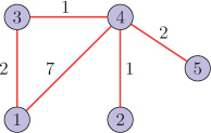
Figure 9.32. Graph G The non-zero eigenvalues of the graph Laplacian are 1.1464, 2.1337, 5.4424, 17.2775. The eigenvector matrix of the Laplacian is

$? = [\begin{matrix} 0.4472 & 0.1840 & 0.2189 & 0.5477 & 0.6467 \\ 0.4472 & - 0.8860 & - 0.0467 & - 0.1036 & 0.0463 \\ 0.4472 & 0.2685 & 0.5663 & - 0.6370 & - 0.0378 \\ 0.4472 & 0.1297 & 0.0529 & 0.4604 & - 0.7540 \\ 0.4472 & 0.3039 & - 0.7914 & - 0.2675 & 0.0987 \end{matrix}]$

1. Consider the graph shown in Figure 9.32.

(a) Calculate Laplacian quadratic forms of all the eigenvectors of the graph Laplacian.

(b) Calculate total variations of all the eigenvectors of the graph Laplacian.

2. For the three graph signals shown in Figure 9.33, which graph signal is likely to have the largest high-frequency components? Why? (All the graph signals are drawn at the same scale).

The three figures are labeled alphabetically and show three graphs G1, G2, and G3. All three have the following network with five nodes labeled from 1 to 5. The first four nodes are placed clockwise such that node 1 becomes the leftmost node. The fifth node is positioned to the right of node 4. The followings nodes are connected: 1 and 2, 1 and 3, 2 and 3, 2 and 4, 3 and 4, and 4 and 5. Vertical lines are extended either upward or downward from each node in all three graphs. The lengths of these lines vary according to their magnitude values. Figure a shows the graph signal for G1 with upward lines form each node. The lengths of the nodes are as follows in the ascending order: 5, 4, 3, 1 and 2. Figure b shows the graph signal for G2 with upward lines form the following nodes: 3, 2, and 4, and downward lines from nodes 5 and 1. The lengths of the lines are in the ascending order. Figure c shows the graph signal for G3 with upward lines form the following nodes: 4, 3, 1, and 2, and downward lines from node 5. The lengths of the lines are in the ascending order.

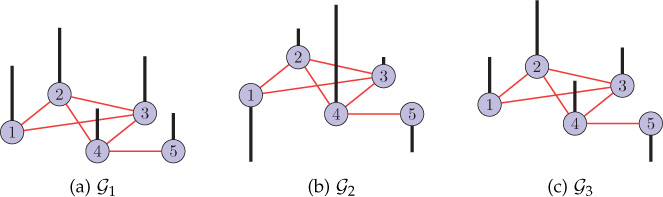
Figure 9.33. Graphs signals (Problem 2)

3. Represent the Laplacian matrix of an undirected graph in terms of impulses defined on the graph.

4. Represent a signal f = [3, 1, 5, − 2, 1]^T defined on graph $?$ , shown in Figure 9.32, as a linear combination of the eigenvectors of the graph Laplacian.

5. The oscillations in a signal lying on a network can also be quantified by the number of zero crossings in the signal values. If there is an edge between nodes i and j and there is a change in the sign of the signal values at nodes i and j, then it is counted as one zero crossing. Create an undirected random network with 300 nodes by adding an edge between any two nodes with a probability of 0.15.

(a) Plot the number of zero crossings in the eigenvectors of the Laplacian matrix with respect to the corresponding eigenvalues. Comment on your observations and explain the frequency ordering.

(b) Repeat part (a) for the normalized Laplacian matrix of the network.

6. Consider two graphs $?_{1}$ and $?_{2}$ having 20 nodes each. Both of the graphs have a common Laplacian eigenvalue 4.5, which also is the largest Laplacian eigenvalue of $?_{2}$ . Is it possible to find a signal defined on graph $?_{2}$ that has a value greater than 2-Dirichlet form of the eigenvector corresponding to the eigenvalue 4.5? Is it possible to find such signal defined on graph $?_{2}$ ?

7. If all the edge weights of graph $?$ shown in Figure 9.32 are doubled, what effect will it have on the following?

(a) The graph frequencies.

(b) The graph harmonics.

What if all the edge weights are halved?

8. Represent the graph signal f shown in Figure 9.34 as a linear combination of impulses, and subsequently find the GFT vector of the signal. The Laplacian eigenvector matrix of the graph is

Figure 9.34. Graph G (Problems 8 and 9)

9. For the graph signal shown in Figure 9.34, compute the gradient vectors at each node. What is the total variation of the graph signal?

10. Consider graph $?$ shown in Figure 9.32. Draw a graph $?'$ by interchanging the vertex labels of nodes 2 and 4. Calculate and plot the following for new graph $?'$ :

(a) Harmonics of the graph.

(b) GFT vector of graph signal f = [3, 1, 5, − 2, 1]^T.

Compare the results with that of graph $?$ .

11. For an undirected graph with the frequencies λ = {0, 1, 2, 4, 5} and the corresponding eigenvector matrix

$? = [\begin{matrix} 0.4472 & 0.2887 & 0 & 0.8165 & 0.2236 \\ 0.4472 & 0.2887 & - 0.7071 & - 0.4082 & 0.2236 \\ 0.4472 & 0.2887 & 0.7071 & - 0.4082 & 0.2236 \\ 0.4472 & 0 & 0 & 0 & - 0.8944 \\ 0.4472 & - 0.8660 & 0 & 0 & 0.2236 \end{matrix}],$

calculate the resulting vector when the graph signal f = [0, 1, −2, 0, 1]^T is operated on by the graph Laplacian; that is, find Lf.

Hint: Represent f as linear combination of the Laplacian eigenvectors.

12. Consider a continuous kernel 2e⁻5λ in graph spectral domain. Corresponding to this kernel, plot the graph signal with its structure being the graph shown in Figure 9.32. For the obtained graph signal, what is the total variation?

Repeat the same for a kernel 2e²λ. What is the total variation for this graph signal? Compare it with the previous result.

13. For the graph shown in Figure 9.32, find a low-pass linear graph filter matrix H that passes frequencies up to 3 and suppresses all the frequency components above 3. For an input graph signal f = [1 , −4, − 6, 2, − 1]^T to the filter, draw the output in the graph spectral domain.

14. Compute and plot the convolution product of two graph signals f = [1, 3, −3, 0, 8]^T and g = [0, 1, −2, 4, 2]^T defined on graph G shown in Figure 9.32.

15. Show that the graph convolution product satisfies the following properties:

(a) It is commutative, that is, f ∗ g = g ∗ f.

(b) It is distributive, that is, f ∗ (g + h) = f ∗ g + f ∗ h.

(d) L(f ∗ g) = f ∗ (Lg) = (Lf) ∗ g.

16. (a) Prove that the operator L^K is localized within K hops at each node, that is, (L^K)_ij = 0for d_G (i, j) > K, where L is the Laplacian matrix of a graph $?$ and d_G (i, j) is the hop distance between nodes i and j. Consequently, show that a polynomial of order K in the Laplacian matrix L is also localized within K hops at each node.

(b) A signal f = [3, 0, 2, 4, 0, 1, 2, 3, 5]^T is defined on the graph $?$ as shown in Figure 9.35. The edge weights a and b are unknown. Consider two polynomial filters

A graph weighted G with nine nodes is displayed.

Figure 9.35. Graph G for Problem 16(b)

(9.10.1) $?_{1} = 2 ? - 2 ?$

and

(9.10.2) $?_{2} = ? + 3 ? - ?^{2} .$

(i) What is the sum of the elements of each row of H₁ and H₂?

(ii) For filter H₁, compute the filtered output at nodes 1, 2, and 3. You should not compute the full Laplacian matrix for finding output at a single node. Just consider the corresponding row of the filter.

(iii) For filter H₂, compute the filtered output at nodes 1 and 3. You should not compute the full Laplacian matrix for finding output at a single node. Just consider the corresponding row of the filter.

(iv) For filter H₁, if the values of the filtered output at nodes 6 and 7 are 4 and 8, respectively, then find the edge weights a and b.

(v) Write down the spectral representations of the filters H₁ and H₂. How many parameters are required to characterize the filters?

17. Considering the graph $?$ shown in Figure 9.32,

(a) Plot the translated versions of a graph signal f = [−1, 6, 2, 0, 3]^T when translated to nodes 2 and 4.

(b) Plot the modulated versions of a graph signal f = [−4, 7, 10, 1, −2]^T when modulated to nodes 1 and 3.

18. Consider two graph signals f = [3, −4, 9, 2]^T and g = [1, 0, −6, 7]^T defined on an arbitrary undirected and connected graph with 4 nodes. If h = f ∗ g, compute $\sum_{i = 1}^{4} ? (i)$ .

19. Consider a graph signal f = [2, −6, 1, −3, 8]^T defined on an arbitrary undirected and connected graph having 5 nodes. Calculate $\sum_{i = 1}^{5} ?_{1} (i)$ and $\sum_{i = 1}^{5} ?_{2} (i)$ , where f₁ = T₁f and f₂ = T₄f.

20. Consider a polynomial kernel of degree K defined in graph frequency domain as

$\hat{?_{K}} (ℓ) = \sum_{i = 0}^{K} a_{i} λ_{ℓ}^{i} .$

Prove that T_ip_K(j) = 0, if d_G(i, j) > K.

21. Consider a graph signal f with its GFT $\hat{?} = δ_{0} (λ_{ℓ})$ , that is, the signal is localized around zero frequency in the graph spectral domain. Prove that when the graph signal f is modulated to frequency λ_k, the resulting graph signal is localized around frequency λ_k, i.e., $\hat{M_{k} ?} = δ_{0} (λ_{ℓ} - λ_{k})$ .

22. Consider a graph signal h defined on an N-node r-regular graph. Let the signal value at a node i be the degree of node i. Answer the following:

(a) Calculate the convolution product h ∗ f, where f is an arbitrary signal defined on the graph.

(b) Prove that the generalized translation operator has no effect on h.

23. Using GSPBox, create a 60-node random sensor network and define a signal f on the graph as

(9.10.3) $? (i) = {\begin{matrix} 10 & if i = 30 \\ 10 e^{- c . d (i, 30)} & otherwise, \end{matrix}$

where c is a constant and d(i, j) is the distance between nodes i and j (can be found using Dijkstra’s shortest path algorithm).

(a) Plot the graph.

(b) For c = 0.05, plot the graph signal in the vertex domain using color coding as well as bar representation. Compute the GFT coefficients, and plot the signal in the frequency domain. Comment on the frequency content of the signal.

(c) Plot the graph signals for c = 0.5, c = 1, and c = 2 in the vertex as well as frequency domains. Comment on the smoothness of graph signals as the value of c increases.

24. Consider the eigenvectors of the normalized Laplacian L^norm as graph Fourier basis. Denote the eigenvalues as ${\bar{λ}}_{ℓ}$ and corresponding eigenvector as ${\bar{?}}_{ℓ}$ . Answer the following:

(a) What is the relationship between ${\bar{?}}_{0}$ and u₀.

(b) For the graph shown in Figure 9.32, write $\bar{?}$ .

(c) For a graph signal f = [9, 0, 2, −4, 5]^T defined on an arbitrary connected graph with the degree matrix D = diag[2, 4, 8, 10, 3], compute $\hat{?} (0)$ .

25. Considering eigenvectors of the normalized Laplacian as the graph harmonics, answer the following:

(a) Plot graph signal f defined in Problem 23(c) for c = 0.1. Compute and plot the GFT coefficients by taking eigenvectors of the normalized Laplacian as the graph Fourier basis. Compare the result with that of eigenvectors of the Laplacian as graph Fourier basis.

(b) Plot the graph signal translated to node 6. (Translation is defined considering normalized Laplacian as graph Fourier basis.)

26. Generate three connected ER graphs: $?_{1}$ (with edge probability of 0.2), $?_{2}$ (with edge probability of 0.25), and $?_{3}$ (with edge probability of 0.3), each having 50 nodes. Define three graph signals: f₁ = u₀ on graph $?_{1}$ , f₂ = u₂₄ on graph $?_{2}$ , and f₃ = u₄₉ on graph $?_{3}$ . Now connect the three graphs by adding six additional edges to form a single connected graph G. Consider signal f = [f₁^T f₂^T f₃^T]^T on graph $?_{1}, f_{2} = u_{24}$ .

(a) Plot the GFT coefficients of signal f. Do they convey any information about the local frequency content of the signal f supported by graphs $?_{1}$ , $?_{2}$ , and $?_{3}$ ? Why or why not?

(b) Plot and explain the spectrogram of graph signal f assuming a heat kernel $\hat{?} (λ_{ℓ}) = a e^{- k λ_{ℓ}}$ ; choose the constants a and k such that ||g||₂ = 1.

An example of an observed graph signal with five nodes.

Figure 9.36. Observed graph signal (Problem 27)

27. This problem demonstrates the use of Laplacian quadratic form for interpolation on graphs. Consider an observed graph signal, shown in Figure 9.36, where signal values at nodes 2, 3, and 4 are missing. The aim of interpolation is to fill in the missing values. One criteria for estimatiing the missing values is to minimize the squared sum of the differences in signal values between the neighboring vertices, which is nothing but the quadratic form of the graph Laplacian. Therefore, the interpolation problem can be written as

(9.10.4) $\begin{matrix} \underset{f}{minimize} \underset{i, j}{Σ} w_{i j} {(f (i) - f (j))}^{2} = f^{T} L f \\ s u b j e c t t o M f = y, \end{matrix}$

where w_ij is the edge weight between nodes i and j, M is a diagonal masking matrix that takes a value of 1 for known indices and 0 for unknown indices, and y is the observed graph signal with zeros at missing indices. For example, if the values at nodes 2, 3, and 4 are missing, the masking matrix is M = diag{1, 0, 0, 0, 1} and the observed graph signal can be written as y = [2, 0, 0, 0, 6]^T. Find the missing values in the observed graph signal by solving the above optimization problem.

Hint: Use the method of Lagrange multipliers.

28. Throughout this chapter, it was assumed that the underlying graph is undirected with non-negative edge weights. Considering the case when the edge weight can be negative or positive, discuss the effect on graph frequencies and their ordering based on the Laplacian quadratic form. What problems might arise in this case?

29. There exist multiple definitions for the Laplacian matrix of a directed graph. Conduct a survey on various Laplacian matrices defined for directed graphs.

1. Note that a different set of real eigenvectors also exists. For example, mathematical software packages such as MATLAB calculate the real set of eigenvectors for symmetric matrices.

2. Also see Exercise Problem 27.

3. Detailed characteristics of ER graphs can be found in Chapter 3.

4. Detailed characteristics of small-world networks can be found in Chapter 4.

5. Detailed characteristics of scale-free networks can be found in Chapter 5.

..................Content has been hidden....................

You can't read the all page of ebook, please click here login for view all page.