Chapter 11
Multiscale Analysis of Complex Networks

In the previous two chapters, we discussed frequency analysis of complex network data using the graph Fourier transform (GFT). Being a global transform, the GFT has the capability of capturing global variations in a graph signal; however, it fails to identify the local vatiations. In classical signal processing, wavelet transforms have been extensively used for extracting local as well as global information from the data. Wavelets have the capability to simultaneously localize a signal content in both time and frequency that allows us to extract information from the data at various scales. Similarly, wavelet-like transforms for network data give us a means to analyze the network data at various scales. Various methods have been developed to design localized, multiscale transforms for analyzing data defined on complex networks. This chapter presents these multiscale techniques for complex network data analysis.

The GFT defined in Chapter 10 is a powerful tool to analyze data defined on complex networks. However, being a global transform, it has certain limitations and drawbacks too. For example, it is highly sensitive to changes in network structures, since a small change (addition or deletion of a few nodes or edges) in the network topology may result in very different eigenvalues and eigenvectors of the graph Laplacian. Moreover, GFT fails to provide any information regarding where in the network topology particular frequency components are present. Although windowed graph Fourier transform gives the answer to where in the network topology particular frequency components are present, it does not localize the signal content in the frequency domain.

In classical signal processing, various techniques are available for wavelet analysis of signals. For continuous time signals, wavelets at different scales are constructed by translating and scaling a single mother wavelet. There also exist second-generation wavelets [197], which are not necessarily composed of either shifts or dilations of some single function. Nevertheless, the wavelets are localized and indexed across a range of scales and locations within scales, have zero integral, and share some common characteristics in their definition. Moreover, for discrete-time signals, there exist discrete wavelet transforms [198] that can be implemented through filterbanks [199] or lifting-based schemes [200].

In the past decade, various techniques have been developed that allow localized multiscale analysis of complex network data. These techniques include the Crovella and Kolaczyk wavelet transform (CKWT) [201], random transform [202], lifting-based wavelets [203], [204], [205], spectral graph wavelet transform (SGWT) [206], two-channel wavelet filter banks [193], and diffusion wavelets [207]. These different approaches derive analogy from different classical multiresolution schemes. For example, SGWT derives analogy from the classical continuous-time wavelet transform, whereas lifting-based wavelets and two-channel wavelet filter banks are the analogues of classical discrete-time wavelet transforms. Although the classical continuous wavelets are time invariant, the graph wavelets are not space invariant due to irregular structure of the underlying graph.

Similar to classical wavelet transform, a graph wavelet transform aims to localize graph signal contents in both the vertex as well as the spectral domains. As described in previous chapters, translation and scaling of graph signals are not straightforward operations. Therefore, the concepts of classical wavelet transforms, where wavelets are constructed by translating and scaling a single mother wavelet, cannot be extended directly in graph settings. Moreover, two-channel wavelet filter banks require downsampling of graph signals, which is not a simple operation. However, these difficulties can be overcome by using the GFT. In the next section, various existing techniques for designing wavelets on graphs are presented.

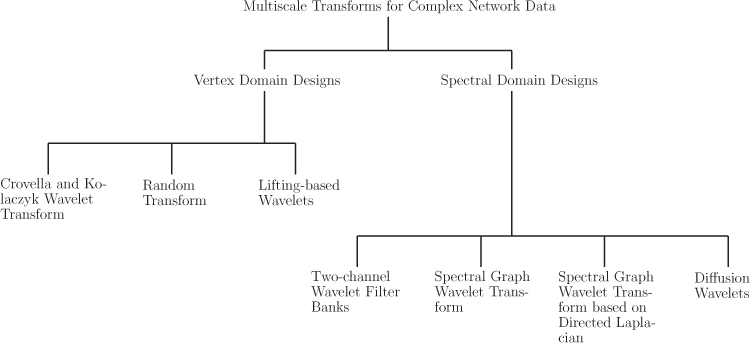
Figure 11.1. Classification of multiscale transforms for data defined on complex networks

In CKWT, the wavelet is constructed based on k-hop distance such that the value of wavelet centered at node i on node j depends only on shortest path distance between nodes i and j. CKWT is designed for unweighted graphs, but inverse transform has not been mentioned.

Random transform [202] was proposed to analyze sensor network data at multiple resolutions.

Lifting-based wavelet transform [203], [204], [205] splits the nodes of a graph into two sets: even and odd nodes. Then, as in standard lifting, data on the nodes of one parity are used to predict/update those of the other. By construction, these transforms are invertible; that is, the graph signal can be found from the transform coefficients.

SGWT is defined by deriving an analogy from the continuous wavelet transform, where wavelets at various scales are derived by translating and dilating a mother wavelet. On the other hand, two-channel wavelet filter banks are analogous to classical discrete wavelet transforms. Diffusion wavelets are orthonormal and use diffusion as a scaling tool for multiscale analysis. In diffusion wavelets, the wavelet construction is based on compressed representations of powers of a diffusion operator. In contrast to diffusion wavelets, SGWT gives precise analogy to classical continuous wavelet transform, gives highly redundant transform, and offers finer control over the selection of wavelet scales. In addition, fast algorithms exist for SGWT computation.

Let us define ?(i,h) as the set of nodes j∈? that are within h-hop distance from node i, that is, d?(i,j)≤h. In addition, let ∂?(i,h) represents the set of nodes j∈? that are exactly at h-hop distance from node i, that is, d?(i,j)=h. The set f nodes ∂ N (i, h) can be considered as an h-hop ring centered around node i. For example, in Figure 11.3, ∂?(1,2) is a two-hop ring centered around node 1 consisting the nodes 5, 6, 7, and 8.

The wavelet ψjiCKWT at scale j and centered around node i is defined as

for some constants {a_jh}_{h=0,1,... ,j} satisfying ∑h=0jajh=0. Also, a_jh = 0, for h > j, and, therefore, the wavelet ψjiCKWT at scale j is supported by exactly a j-hop circle around node i. From Equation 11.3.1, we can observe that a wavelet is constant in an h-hop ring centered around node i and depends on the distance h from the center node.

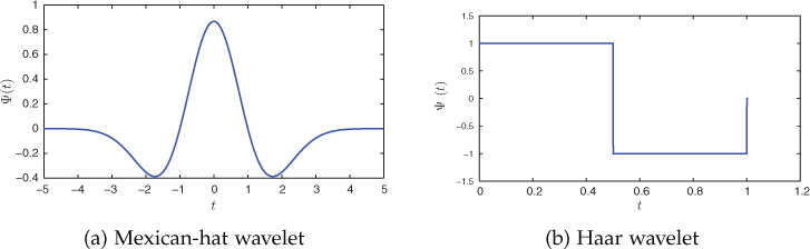
Figure 11.2. Continuous-time Mexican-hat and Haar wavelets

where I_jh = [h/(j + 1), (h + 1)/(j + 1)] is one of the equal-length subintervals over [0,1].

These coefficients for a graph signal at different scales can be utilized to extract useful information, for example, the spread of the graph signal localized to a particular node.

1. A CK wavelet has zero mean, that is, ∑k=1NψjiCKWT(k)=0, where ψjiCKWT is a graph wavelet at scale j and centered at vertex i.

2. A CK wavelet at scale j and centered at vertex i (ψjiCKWT) has constant value at the nodes that are equidistant from center node i. That is, ψjiCKWT(k)=ψjiCKWT(l), if d?(i,k)=d?(i,l)≤j. This property of symmetricity can be visualized from an example graph shown in Figure 11.3. A wavelet centered at node 1 will have equal values at nodes 2, 3 and 4 that are at one-hop distance from the center node 1. Also, the wavelet has equal values at nodes 5, 6, 7, and 8, which are at two-hop distance from the center node.

3. A CK wavelet at scale j and centered at vertex i (ψjiCKWT) has zero value at the nodes that are not within j-hops from center node i. That is, ψjiCKWT(k)=0, if d?(i,k)=d?(i,l)≤j.

Figure 11.3. Illustration of symmetricity property of a graph wavelet in CKWT scheme

Table 11.1. Computing a_jh for the network shown in Figure 11.3 (assuming ψ(t) as Haar wavelet)

Having found the values of coefficients a_jh, we can compute wavelets centered at the desired node using Equation (11.3.1). For example, CK wavelets centered at node 1 and scales j = 1, 2 are

The two different basis functions under this framework are weighted average basis functions and weighted difference basis functions. A weighted average basis function at scale h and centered at node i is represented by ψ_hi. It computes the weighted average on the h-hop neighborhood of node i, giving more weight to the value at node i. Let ∂?(i,h) represents the set of nodes j∈? that are within h-hop distance from node i, that is, d?(i,j)≤h. Defining the h-hop degree of node i as di,h=|?(i,h)|, the weighted average basis function at scale h and centered at node i is given as

where 0<a<12 is a constant and ?(i,h)i denotes the set of nodes ?(i,h) excluding node i.

A weighted difference basis function at scale j and centered at node i is represented as φ_hi. It computes the weighted difference of the value at node i and the values at its h-hop neighbors. It is given by

where b > 0 is a constant.

The set of weighted average basis functions at scale h can be represented in matrix form as Ψ_h = [ψ_h1, ψ_h2,... ,ψ_hN], and the set of weighted average basis functions at scale h can be represented in matrix form as Φ_h = [φ_h1, φ_h2,... ,φ_hN]. It is worth noting that for any non-negative integer value of h∈ℕ, the set of weighted average (or weighted difference) graph-dependent functions {ψ_h1,_h2,... , ψ_hN} (or{φ_h1, φ_h2,... , φ_hN}) forms a basis for a graph signal ℝN over any finite undirected graph.

By changing the scale h, we can compute basis functions with different support on the graph, and subsequently these basis functions can be utilized to analyze data, such as sensor network data, at multiple resolutions. Intuitively, this approach defines a two-channel wavelet filter bank on the graph consisting of two types of linear filters: (i) approximation filters (given by Equation (11.4.1)) and (ii) detail filters (given by Equation (11.4.2)).

In standard lifting, a discrete-time signal is first split into two sequences: even sequence and odd sequence. Similarly, in order to apply the lifting-based transform to an arbitrary graph signal, we need to split the nodes ? of the graph into even and odd sets of nodes. However, splitting of a graph into two clusters imposes a great challenge because of irregular nature of the graph.

Let us consider that the algorithm results in m number of odd nodes and n number of even nodes, where m + n = N. The graph signal f and the adjacency matrix of the graph ? are then arranged as

where submatrix S^o is the adjacency matrix of the subgraph containing odd nodes and S^e is the adjacency matrix of the subgraph containing even nodes. These matrices contain edges which have conflicts, since they connect nodes of the same parity. The block matrices P and Up contain edges which do not have conflicts. The matrices P and Up are used to design prediction and update filters, respectively, for lifting-based transform. Note that a good even-odd splitting of a graph should minimize the edge information present in the matrices S^o and S^e (thus minimizing the number of conflicts).

Figure 11.4. Block diagram of lifting-based transform

The lifting-based transform outputs two vectors f₁ and d₁ for an input graph signal f. The vector f₁ is analogous to the approximation sequence of standard lifting transform and the vector d₁ is analogous to the detail sequence of standard lifting transform. The lifting-based wavelet transform on a graph can be performed by using the following equations:

where ?? is the prediction filter and ?? is the update filter. The prediction filter matrix ?? is computed from the matrix P of Equation (11.5.1) by multiplying each row with prediction weights. Similarly, the update filter matrix ?? is computed from matrix Up by multiplying each row with update weights.

The lifting-based transform is invertible by its construction. The inverse transform can be calculated using the following equations:

Depending on the application, we can perform multiple lifting operations on the updated set of even nodes. Starting from scale j = 1, one-step lifting results in the even set of nodes ?1 and odd set of nodes ?1. In a two-step lifting, the lifting operation is again performed on the even set of nodes ?1 to obtain even set of nodes ?2 and odd set of nodes ?2.

As discussed in Chapter 8 (Section 8.5.6), bipartite graphs exhibit a spectral folding phenomenon, which allows one to design perfect reconstruction wavelet graph filter banks known as graph quadrature mirror filter banks (graph-QMFs) for bipartite graphs. Moreover, for arbitrary graphs, two-channel filter banks are constructed in cascade, along a series of bipartite subgraphs of the original graph.

In the discussion of two-channel graph wavelet filter banks, the normalized form of Laplacian ?norm=?−12??12 is used. A detailed discussion on normalized Laplacian can be found in Chapter 2.

A two-channel graph filter bank constitutes downsamplers and upsamplers. Therefore, first we discuss downsampling and upsampling operations over graphs.

To downsample a graph signal, first we need to find a set of nodes ℋ and then discard the samples of the original graph signal at this set of nodes. A downsampler for graph signals is shown in Figure 11.5. It is characterized by a downsampling function βℋ, where ℋ⊂? is the set of nodes to be discarded by the downsampling operation. The output of the downsampler is a graph signal ?d∈ℝN−|ℋ| that retains the values of the original graph signal at the set of nodes ℋc=?−ℋ. The downsampling function βℋ is defined as

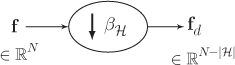
Figure 11.5. A downsampler for graph signals

An upsampler characterized by βℋ is shown in Figure 11.6. The upsampler projects a downsampled graph signal ?d∈ℝN−|ℋ| back to original ℝN by inserting zeros at the set of nodes ℋ.

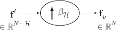
Figure 11.6. An upsampler for graph signals

A cascaded block consisting of a downsampler followed by an upsampler is shown in Figure 11.7. This cascaded structure is common in graph filter banks. Overall, it performs downsample then upsample (DU) operation. Let us define a downsampling matrix ?βℋ=diag{βℋ(n)}. For a graph signal f as the input to the cascaded blocks, the DU output is given by

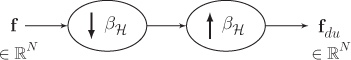
Figure 11.7. A downsampler and an upsampler in cascade

where I_N is an N × N identity matrix and

Since ?βℋ is a diagonal matrix, ⟨?ℓ,?βℋ?⟩=⟨?βℋ?ℓ,?⟩. Therefore, Equation (11.6.4) can be written as

In this equation, observe that the first term is the GFT coefficient of the input graph signal at the corresponding frequency λ_l, whereas the second term is the deformation component. Let us represent the deformed harmonic at frequency λ_ℓ as ?ℓd=?βℋ?ℓ. Hence, the second term in Equation (11.6.5) can be called a deformed spectral coefficient, which is the projection of the input graph signal onto the deformed eigenvector (harmonic) ?ℓd. Now, the GFT coefficient of the DU graph signal can be written as

where f^d(λℓ)=?T?ℓd is the deformed spectral coefficient at frequency λ_ℓ.

In simple form, the spectrum of the DU graph signal can be written as

where

is the deformed spectrum of signal f. Note that ?d=?βℋ? is the deformed graph Fourier basis.

---

Example 11.6.1

This example illustrates the DU operation. Consider the bipartite graph shown in Figure 11.8(a). The eigenvalues of the normalized graph Laplacian are shown in Figure 11.8(b). Now consider a signal f = [−2, 3, −2, 5, 1, −3, 1]^T defined on the graph. Let us assume that we downsample the signal by discarding a set of nodes ℋ={5,6,7}. Therefore, the downsampling matrix for a DU operation is given by ?βℋ=diag{1,1,1,1,−1,−1,−1} and the DU signal becomes f_du = [−2, 3, −2, 5, 0, 0, 0]^T.

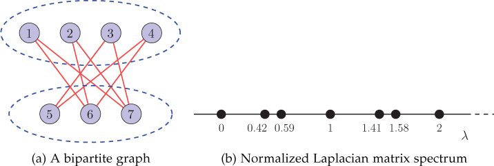
Figure 11.8. A bipartite graph and its normalized Laplacian matrix spectrum

The matrices containing the graph Fourier basis U and the deformed graph Fourier basis ?d=?βℋ? as their columns are

?=[0.35360.353600.707100.35360.35360.35360.35360−0.707100.35360.35360.3536−0.3536−0.50000−0.5000−0.35360.35360.3536−0.35360.500000.5000−0.35360.35360.3536−0.61240000.6124−0.35360.43300.25000.50000−0.5000−0.2500−0.43300.43300.2500−0.500000.5000−0.2500−0.4330]

and

(11.3.9) ?d=[0.35360.353600.707100.35360.35360.35360.35360−0.707100.35360.35360.3536−0.3536−0.50000−0.5000−0.35360.35360.3536−0.35360.500000.5000−0.35360.3536−0.35360.6124000−0.61240.3536−0.4330−0.2500−0.500000.50000.25000.4330−0.4330−0.25000.50000−0.50000.25000.4330].

The spectrum of signal f and the spectrum of its DU version f_du are plotted in Figures 11.9(a) and (b), respectively. Since the underlying graph is bipartite, notice that the spectrum ?^du is symmetric about frequency λ = 1. This symmetricity results from a phenomenon known as spectral folding, described next.

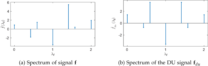
Figure 11.9. Spectra of signal f defined on the bipartite graph shown in Figure 11.8(a) and its DU version

As discussed in Chapter 8, the spectrum of normalized Laplacian for bipartite graphs is symmetric about 1. This symmetry property is responsible for the phenomenon of spectral folding in bipartite graphs: if u_ℓ is an eigenvector of L^norm corresponding to the eigenvalue λ _ℓ, then the deformed eigenvector ?ℓd=?β?ℓ is also an eigenvector of L^norm with an eigenvalue 2 − λℓ . Note that the downsampling function β chosen here is βℋ or βℒ as given by Equation (11.6.1).

Using Equations (11.6.5) and (11.6.6), for bipartite graphs, we can write

The above equation can be interpreted as follows. In the spectral domain, the result of a DU operation over a bipartite graph is the average of the original graph signal and an aliasing term which is the folded version of original signal with respect to λ = 1.

A two-channel graph wavelet filter bank decomposes a graph signal (?∈ℝN into a low-pass (smooth) component (?ℒ∈ℝN and a high-pass (detail) component (?ℋ∈ℝN. The filter bank is called a perfect reconstruction graph filter bank if the sum of the low-pass and high-pass components is same as the input graph signal. From Figure 11.10, the low-pass and high-pass components can be written as

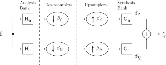
Figure 11.10. Two channel filter bank on graph

The reconstructed signal is the sum of these two signal components:

In the above equation, Term 1 is the equivalent operator for the system without the DU operation. Term 2 is an aliasing term that comes from the DU operation. For perfect reconstruction, Term 2 should be zero and Term 1 should be an identity matrix. Therefore, perfect reconstruction is possible if

where c is a scalar constant, and

In case of bipartite graphs, consider βℒ=β and βℋ=−β. Then, for a bipartite graph, the condition given by Equation (11.6.14) can be rewritten as

The above conditions are incorporated for designing a graph-QMF, which is described next.

and

Here, g₀, g₁, h₀, and h₁ are kernels (in spectral domain) corresponding to the filters G₀, G₁, H₀, and H₁, respectively. One possible choice for the filter kernels is [193]

for any arbitrary kernel h₀(λ _ℓ).

Therefore, for a bipartite graph ? with its two partitions as ℋ and ℒ, with a downsampling function β=βℋ in a two-channel filter bank, as shown in Figure 11.10, the filter kernels given by Equation (11.6.18) guarantee perfect reconstruction for any arbitrary kernel h₀(λ_ℓ).

Once the set of bipartite subgraphs is obtained, graph-QMFs can be implemented for each of these subgraphs in a cascaded manner. At every stage, filtering operations are done along one dimension using only the edges that belong to the corresponding bipartite subgraph. This approach is a separable approach in the sense that results of the transform in one stage are used in the next stage. Figure 11.11 shows a 2-D two-channel filterbank. Here, a graph is decomposed into two bipartite subgraphs ℬ1 and ℬ2. In the first stage, edges of subgraph ℬ1 are utilized, and at the second stage, edges of subgraph ℬ2 are utilized.

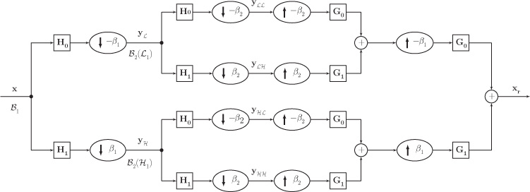
Figure 11.11. Two channel filter bank on an arbitrary graph

1. See Appendix B.6 for details on continuous-time wavelets.

Note that scaling ψ by 1/s corresponds to scaling ψ^ with s and the modulation term e^−jωa comes from localization of the wavelet at location a. Thus, a wavelet can be interpreted as an inverse Fourier transform of the scaled and modulated band-pass filter ψ^.

Analogous to the Fourier representation of classical continuous wavelets, spectral graph wavelets are constructed based on a kernel g defined in the graph Fourier domain. Kernel g behaves as a band-pass filter; that is, it satisfies g(0) = 0 and lim_x→∞ g(x) = 0. The spectral graph waveletψ_t,n, at scale t and centered at node n, is defined through spectral decomposition of the graph Laplacian matrix L (symmetric) as

Here, in comparison to the classical wavelet described by Equation (11.7.1), frequency ω is replaced with the eigenvalues of the graph Laplacian λ_ℓ. Furthermore, translating (or localizing) a wavelet to node n corresponds to a multiplication by uℓ*(n), replacing e−jωa, replacing e⁻ jωa. In addition, g acts as a scaled bandpass filter, replacing ψ^ of Equation 11.7.1. One important point to note here is that the spectral wavelets are continuous in scale but discrete in space. The filter kernel function g is defined as a real-valued continuous function defined on ℝ+ and sampled at the discrete frequency values of (λ_ℓ) _ℓ=0,... ,N−1. In practical scenarios, to have a finite number of scales, the continuous scaling parameter t is also sampled; that is, a total of J scales are considered: {t_j}_j=1,... ,J.

where G_t = diag[g(tλ₀), g(tλ₁),... , g(tλ_N−1)] is a diagonal matrix with the diagonal entries as values of the scaled band-pass filter sampled at the graph frequencies. Therefore, the wavelet (column) vector at scale t and centered at node n is

Hence, the wavelet basis at scale t, which is the collection of N number of wavelets (each wavelet centered at a particular node of the graph), can be written as

Now, the wavelet coefficient at scale t and centered at node n of a graph signal f can be calculated as

SGWT can be computed efficiently using the fast Chebyshev polynomial approximation algorithm [206], which avoids full eigendecomposition of the graph Laplacian matrix.

where x is the distance from origin (zero frequency), α and β are integer parameters of the band-pass filter g, x₁ and x₂ determine transition regions, and p(x) is a 3-D cubic spline that ensures continuity in g. One possible choice of these parameters can be α = β = 2, x₁ = 1, x₂ = 2, and p(x) = −5 + 11x − 6x² + x³.

A total of J logarithmically equally spaced discrete wavelet scales can be selected for practical purposes: t₁,... , t_J, where t_J is the minimum scale. Considering λ_min = |λ_max|/K, where λ_max is the eigenvalue of L with the largest magnitude and K is a design parameter, we set t_J = x₂/|λ_max| and t₁ = x₂/λ_min.

Kernels for different scales with parameters |λ_max| = 7.8830, α = β = 2, x₁ = 1, x₂ = 2, K = 20, and J = 4, are shown in Figure 11.12. Figure 11.12(a) shows original kernel (t = 1). Kernels at scales t = 5.0742, t = 1.8693, t = 0.6887, and t = 0.2537 are shown in Figures 11.12(b), (c), (d) and (e), respectively. One can clearly observe that kernels become increasingly confined to low frequencies with the increase in scale t.

Figure 11.12. Kernels at various scales. As the scale t increases, the kernel becomes increasingly confined to low frequencies.

Figure 11.13. An arbitrary network

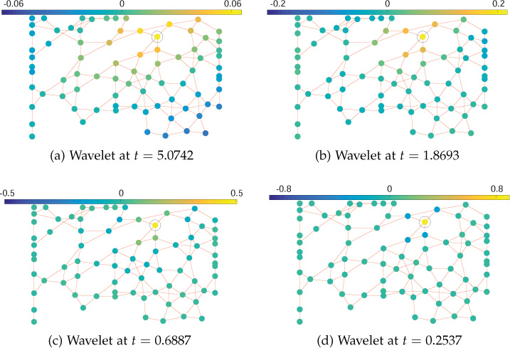
Figure 11.14. Wavelets at various scales for an arbitrary network. Wavelets are centered around the circled node.

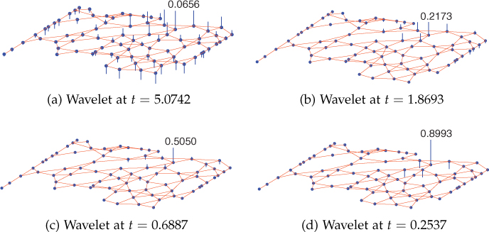
Figure 11.15. Another representation of the wavelets plotted in Figure 11.14

SGWT has been used in various applications, including mobility inference [210] and community mining [211]. SGWT can be used in the analysis of network dynamics for capturing and quantifying the changes as well.

However, SGWT is not applicable to directed graphs. Also, SGWT is highly sensitive to network topology: a small change in network topology can alter the wavelets significantly. This is because the eigenvalues and eigenvectors of the graph Laplacian are highly sensitive to the network topology.

where V is the graph Fourier basis described in Section 10.5.5, G_t = diag[g(tλ₀), g(tλ₁),... , g(tλ_N−1)], and g(tλ_ℓ) is the value (real) of scaled 2-D generating kernel at graph frequency λ_ℓ (complex). Therefore, wavelet at scale t and centered at node n is

where ?_n is an N-dimensional column vector having unit value only at the n^th entry and zero elsewhere. Furthermore, the wavelet transform coefficient of a graph signal f at scale t and node n can be calculated as

where r=x2+y2 is the distance from origin (zero frequency), α and β are integer parameters of the band-pass filter g, r₁ and r₂ determine transition regions, and p(r) is a 3-D cubic spline surface that ensures continuity in g. The parameters used are same as in [206]: α = β = 2, r₁ = 1, r₂ = 2, and p(r) = −5 + 11r − 6r² + r³.

A total of J logarithmically equally spaced discrete wavelet scales can be selected for practical purposes: t₁,... , t_J, where t_J is the minimum scale. Considering λ_min = |λ_max|/K, where λ_max is the eigenvalue of L with the largest magnitude and K is a design parameter, the wavelet scales can be set as t_J = r₂/|λ_max| and t₁ = r₂/λ_min.

Kernels for different scales with parameters |λ_max| = 2.2871, α = β = 2, r₁ = 1, r₂ = 2, K = 20, and J = 4 are shown in Figure 11.16. The four scales have been chosen such that they are logarithmically equally spaced between t_J = x₂/|λ_max| and t₁ = x₂/λ_min. One can clearly observe that kernels become increasingly confined to low frequencies with the increase in scale t.

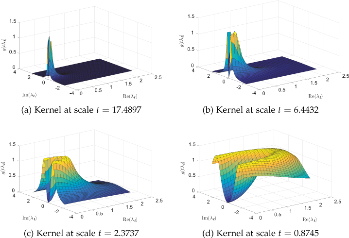
Figure 11.16. Kernels at different scales. As the scale t increases, kernels become increasingly confined to low frequencies. Only the positive real-half of the frequency plane is shown for ease of visualization.

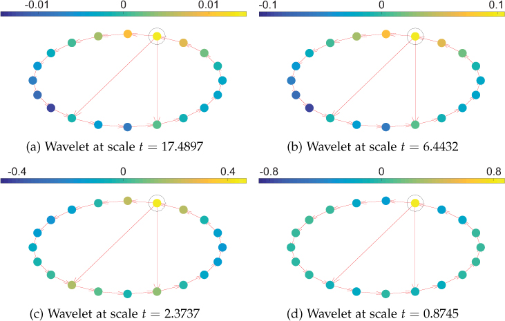
Figure 11.17. Wavelets on directed ring graph. Wavelets at different scales centered at the circled node. As the scale t decreases (high frequencies dominate), the wavelet spread also decreases.

As a second example, a directed weighted graph is constructed from the undirected Minnesota road network. The original road network is made directed by arbitrarily assigning directed weights to some of the edges (22 edges) of the undirected network. Figure 11.18 shows wavelets on this directed network. It can be observed that the spread of the wavelets decreases as scales decrease.

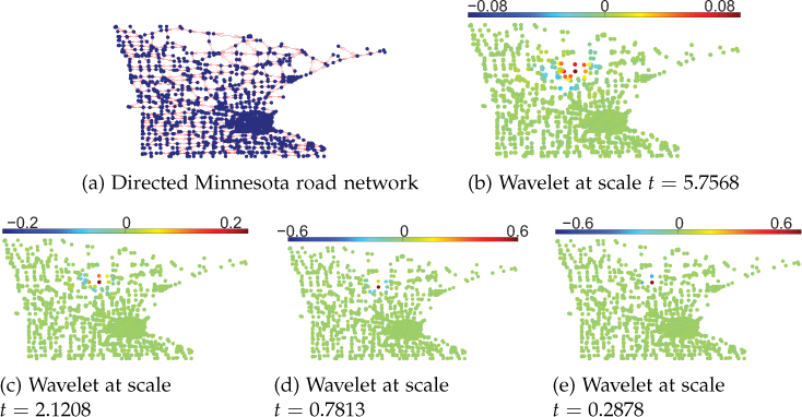
Figure 11.18. Wavelets at different scales centered at the circled node. As the scale t decreases (high frequencies dominate), the wavelet spread also decreases.

Diffusion wavelets not only produce wavelets on complex networks but also produce coarser versions of a complex network, allowing multiscale analysis of complex networks. The graphs (complex networks) encountered in the present time are very large. Usually the finest-scale information contained in a graph is noisy. Therefore, a graph at the finest scale is not always the most informative for a specific task. By compressing graphs at multiple scale, we can reduce the size of a graph in a meaningful way. Compressing a graph means to produce coarser and coarser graphs that replicate the original graph at different levels of resolution. The framework of diffusion wavelets provides a means to compress a graph.

The diffusion operator T utilized in this scheme is the random walk matrix, ?=?12??−12, where D is the degree matrix and W is the weight matrix of the graph. Note that the dyadic power of T are utilized. The powers T^2j (for j > 0) describe the behavior of the diffusion at different scales. As the power of T is increased, the spectrum shift toward zero; that is, more and more eigenvalues tend to be small. In other words, high powers of T are low rank and, therefore, it allows compression by efficiently representing them on an appropriate basis. It is important to note the consistency in the compression in the diffusion operator is defined such that one step of the random walk at scale j corresponds to 2^j+1 steps of the original random walk. The basis functions used here are not the eigenvectors of the diffusion operator T, but are the localized basis functions obtained from the QR decomposition. The reason behind not using the eigenvectors as the basis is that they are global over the graph and, therefore, are unable to give any local information.

The localized basis functions at each resolution level are orthogonalized and downsampled appropriately to transform sets of orthonormal basis functions through a variation of the Gram-Schmidt orthonormalization (GSM) scheme. Although this local GSM method orthogonalizes the basis functions (filters) into well localized bump functions in the spatial domain, it does not provide guarantees on the size of the support of the filters it constructs.

While an orthogonal transform is desirable for many applications, for example, signal compression, the use of the orthogonalization procedure complicates the construction of the transform. Moreover, the relation between the diffusion operator T and the resulting wavelets is not directly evident.

• Two-channel wavelet filter banks guarantee perfect reconstruction for bipartite graphs only. For artibtary graphs, it requires the original graph to be decomposed into a series of separable bipartite subgraphs. However, this decomposition is not unique, and the question remains open about which decomposition is better than other methods.

• M-channel filter banks on graphs have been developed in [194] and [195]. However, perfect reconstruction is guaranteed only for a class of graphs with certain conditions. Development of filter banks on arbitrary graphs that achieve perfect reconstruction is an interesting area to investigate.

• Although SGWT closely resembles the classical countinuous-time wavelet transform, the wavelets in this scheme do not follow the shift-invariance property as do classical wavelets. Graph wavelets with the shift-invariance property might be an interesting problem to investigate.

• Properties of SGWT_DL have not been studied, nor has the inverse transform been presented. Also, the effect of edge directivity has not been investigated.

• All of the multiscale transforms presented in the chapter utilize only the underlying graph structure and do not take the properties of the signal into consideration. For images and multidimensional regular signals, a number of wavelet transforms exist that take signal properties into consideration [212]. Constructing signal-adaptive wavelets on graphs is a challenging area of research. Some efforts in this direction can be found in [213].

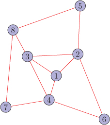
Figure 11.19. Graph G

The non-zero eigenvalues of the graph Laplacian are 1.1464, 2.1337, 5.4424, 17.2775. Moreover, the eigenvector matrix of the Laplacian is

1. For the graph shown in Figure 11.20, compute CK wavelets centered at node 2 at all possible scales. Assume Haar wavelet as ψ(t). Also verify the properties of the CK wavelets listed in Section 11.3.3.

Figure 11.20. Graph for Problem 1

2. In Example 11.6.1, assume that nodes 1, 2, 3, and 4 are discarded. Write down the deformed graph Fourier basis and plot the spectrum of DU signal.

3. Consider the graph shown in Figure 11.21(a).

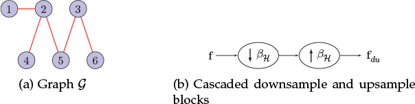
Figure 11.21. Graph and DU blocks (Problem 3)

(a) Is the graph bipartite? If yes, write down the nodes belonging to the two sections of the graph and denote them as ℋ and ℒ.

(b) Explain the spectral folding phenomenon exhibited by the graph ?.

(c) For the cascaded downsample upsample block shown in Figure 11.21(b), find the downsampling matrix. Compute the DU output for an input graph signal f = [4, −7, 1, −2, 3]^T.

(d) Represent the GFT coefficients of the output DU graph signal in terms of input and deformed spectral coefficients.

4. Consider the same graph as in Problem 3 if the output signal to the block diagram shown in Figure 11.22 is f_out = [−2, −1, 3, 9, 0]^T. Compute the input signal f_in.

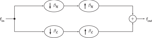
Figure 11.22. Block diagram for Problem 4

5. In Figure 11.10, assume that the filter H₀ is charaterized in spectral domain as

Assuming that the underlying structure for the input signal f is a bipartite graph, plot the kernels in the spectral domain for the filters H₁, G₀, and G₁ so that perfect reconstruction condition is satisfied.

Considering a signal f = [−2, 1, 9, 0, 4, −5]^T defined on the graph G shown in Figure 11.21(a), find the signals at the output of each block in Figure 11.10 and verify that perfect reconstruction is achieved.

6. For the graph shown in Figure 11.19, compute the wavelets centered at node 1 and at scales t = 2, 10, and 40. Use the same kernel given by Equation (11.7.7). Comment on the wavelets at different scales.

7. This problem is about detecting anomalous nodes in a sensor network. Using GSPBox, create a 60-node random sensor network and define a signal f on the graph as

where c = 0.1 is a constant and d(i, j) is the distance between nodes i and j (can be found using Dijkstra’s shortest path algorithm). This signal can be thought of as temperature values in a geographical area, since the variations in temperature values are not high if the sensors are placed densely. Now introduce some anomaly in the graph signal by making the temperature values zero for sensors 18 and 39.

In Problem 12 of Chapter 10, the anomaly can be detected using GFT; however, one could not locate the anomalous nodes. Use SGWT to find the anomalous nodes from the temperature data you created. Write down the step-by-step procedure and explain why your procedure works.

8. This problem is about quantifying spread of a graph signal. The spread of a graph signal can be defined in the vertex as well as the spectral domains. In the vertex domain, the spread of a signal f lying on a graph G about a node v_i is defined as

where P_vi = diag{d(v_i, v₁), d(v_i, v₂),... d(v_i, v_N} is a diagonal matrix with d(v_i, v_j) being geodesic distance between nodes v_i and v_j. Moreover, the overall graph spread (or simply graph spread) is the minimum of the graph spreads about all the nodes, that is,

The spectral spread of a graph signal f is defined as

where L is the Laplacian matrix of the graph.

Based on the graph and spectral spread definitions, answer the following:

(a) Prove that

     where f^(λℓ) is the GFT coefficient at frequency λ_ℓ.

(b) Write an expression for spectral spread of the eigenvectors of the graph Laplacian. What is the relation between the spread of the eigenvectors?

(c) For the graph shown in Figure 11.19, find graph spreads of the eignevectors of the Laplacian matrix. Can you find a relation between the graph and spectral spreads of the eigenvectors?

(d) Compute the graph and spectral spreads for an impuse signal δ_i.

9. Based on the definitions of spread in Problem 8, compute the graph and spectral spreads of the wavelets found in Problem 6. Comment on the graph and spectral spreads of the wavelets at different scales.