10 Graph Signal Processing Approaches

Search in book...
Toggle Font Controls
Create new playlist

Name your new playlist

Playlist description (optional)
Sign In

Email address

Password

Forgot Password?

or

Continue with Facebook

Continue with Google
Sign Up

Full Name

Email address

Confirm Email Address

Password

or

Continue with Facebook

Continue with Google

Chapter 10
Graph Signal Processing Approaches

The last chapter presented extension of classical signal processing operations such as convolution, translation, filtering, and modulation to the signals supported by complex networks. These operators were defined through graph Fourier transform (GFT). The GFT was defined by considering the eigenvectors of the (sym-metric) graph Laplacian matrix as the graph harmonics. In this approach to graph signal processing (GSP), the graph Laplacian played a fundamental role. However, GSP is not limited to the approach based on the graph Laplacian. There exist various approaches for GSP that define the GFT differently. For example, discrete signal processing on graphs (DSP_G) approach is equipped with the theory of linear shift invariant (LSI) graph filters and defines the GFT such that the graph Fourier bases are the eigenfunctions of LSI graph filters. The GFT aimed at frequency analysis of graph signals facilitates efficient handling of the data and remains at the heart of every GSP approach. In this chapter, we discuss some of the existing approaches for GSP.

10.1 Introduction

There exist two major approaches for GSP: (i) GSP based on Laplacian and (ii) the DSP_G framework.

One of the approaches for GSP is the Laplacian-based approach, which was discussed in Chapter 9. In this approach, the Laplacian matrix of the graph plays a fundamental role. The eigendecomposition of the (undirected) graph Laplacian was used to define the GFT, and Laplacian quadratic form was used to identify low and high frequencies. Basic operators such as convolution, translation, modulation, and dilation were defined through GFT. Moreover, windowed graph Fourier transform (WGFT) was also defined for analyzing local frequency components in a graph signal. WGFT was defined through generalized translation and modulation operators. The drawback of this approach is that it is limited to undirected graphs with positive edge weights.

The second approach, the DSP_G framework [177][178] is rooted in the algebraic signal processing theory. In this framework, a shift operator is defined on the graph and plays a fundamental role. Based on the shift invariance, the concept of LSI filtering has been developed. A linear graph filter, which is a matrix operator, is called shift invariant if shifting and filtering operations can be done in any order without altering the filter output. Furthermore, to define the GFT, the eigenvectors of a graph structure matrix are used as the graph harmonics, and the corresponding eigenvalues act as the graph frequencies. The high and low frequencies of the graph are identified through the graph total variation of the eigenvectors. The total variation is defined with the help of the shift operator. This approach is applicable to undirected as well as directed graphs with real or complex edge weights.

10.2 Graph Signal Processing Based on Laplacian Matrix

The Laplacian-based approach is limited to the analysis of graph signals lying on undirected graphs with real nonnegative weights. In this framework, various transforms including GFT, WGFT, spectral graph wavelet transform (SGWT), and wavelet filter banks have been introduced. Among these transforms, GFT remains central because it provides frequency interpretation of a graph signal and, therefore, other transforms have been derived from it. In GFT, a graph signal is represented as a linear combination of the eigenvectors of the graph Laplacian matrix L that is assumed to be symmetric and thus constitutes a complete set of orthonormal real eigenvectors. The eigenvectors act as the graph harmonics, the corresponding (real) eigenvalues of L act as the graph frequencies. Mathematically, GFT of a graph signal f is defined as fˆ=UTf $\hat{?} = ?^{T} ?$ , where U = [u₀ u₁ ... u_N₋₁] is the matrix in which columns are the eigenvectors of L. Here, the frequency ordering is based on the quadratic form and turns out to be natural; that is, small eigenvalues correspond to low frequencies, and vice versa. Additionally, inverse GFT can be calculated as f=Ufˆ $? = ? \hat{?}$ . However, in case of directed graphs, this approach fails since the eigenvectors of the graph Laplacian no longer remain orthogonal and signal recovery from the transform coefficients becomes impossible.

10.3 DSP_G Framework

The roots of the DSP_G approach lie in the algebraic signal processing (ASP) theory [179], [180]. The ASP theory is a formal, algebraic approach to analyze data indexed by special types of line graphs and lattices. The theory uses an algebraic representation of signals and filters as polynomials to derive fundamental signal processing concepts such as shifting, filters, z-transform, spectrum, and Fourier transform. ASP theory was also extended to multidimensional signals and nearest neighbor graphs and was applied in signal compression. The DSP_G framework is a generalization of ASP to signals on arbitrary graphs. In this chapter, the ASP theory is not discussed in detail; the DSP_G framework is self-contained and can be understood without the details of ASP theory. Also, to keep the explanation simple, we have avoided the algebraic model in our presentation of the framework. Interested readers can refer to the research papers.

The DSP_G framework has been built on a graph shift operator. The relationship between the concepts developed under DSP_G is shown in Figure 10.1. The concept of LSI filters is extended to graph settings through the shift operator. Further to define the GFT, the graph Fourier bases are selected such that they are eigenfunctions of LSI filters. Based on the selection of shift operator, one can choose a graph representation (structure) matrix whose eigendecomposition is used to define the GFT. The eigenvalues of the graph representation matrix are treated as graph frequencies and the corresponding eigenvectors as graph harmonics. To identify the low and high frequencies, a quantity called total variation (TV) is defined that quantifies variations in a graph signal. The shift operator is used to define TV on graphs, which is subsequently utilized for ordering of graph frequencies. Based on the TV values of the eigenvectors of the graph representation matrix, the low and high frequencies are identified. Eigenvectors with low TV value correspond to low frequencies, and vice versa.

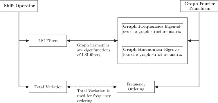
Diagrammatic representation of the relationship between the different concepts under the DSP subscript G framework.

Figure 10.1. Relationship between different concepts under the DSP_G framework

10.3.1 Linear Graph Filters and Shift Invariance

Filtering is a fundamental operation for processing of graph signals. A linear graph filter is characterized by a matrix H∈CN×N $? \in ℂ^{N \times N}$ , where N is the number of nodes in the graph. It is a linear system which takes a graph signal as input and outputs the filtered graph signal. The filter H represents a linear system because the filter’s output for a linear combination of input signals f₁ and f₂ equals the linear combination of the outputs to each signal:

(10.3.1) H(af1+bf2)=aHf1+bHf2, $? (a ?_{1} + b ?_{2}) = a ? ?_{1} + b ? ?_{2},$

for some scalars a and b. Figure 10.2 shows a graph filter, where f_in is the input to the filter H and f_out is the filtered output.

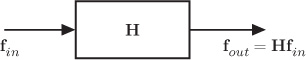
Figure 10.2. A graph filter

In DSP_G, the shift operator S is an elementary linear filter. Using the shift operator, the classical theory of LSI filters can be extended to graph signals. A linear graph filter is called shift invariant if shifting and filtering operations can be done in any order without changing the filter output. In other words, a filter H is shift invariant if the output to the shifted input is equal to the shifted output. That is, the filter H is shift invariant if it satisfies

(10.3.2) S(Hf)=H(Sf). $? (? ?) = ? (? ?) .$

Therefore, for a shift invariant filter, the shift operator and the filter matrix should commute, that is,

(10.3.3) SH=HS. $? ? = ? ? .$

Note that not every linear filter can be shift invariant.

Eigenfunctions of LSI Filters

If the output of an LSI graph filter is only a scaled version of the input, the input is called an eigenfunction of the LSI filter. Consider a graph signal f_in as input to an LSI filter H. If output of the filter is only a scaled version of the input, that is, f_out = Hf_in = αf_in for some scalar α, then the input is an eigenfunction of the filter.

If the input to an LSI filter is represented as a linear combination of its eigenfunctions, then the output can also be represented as a linear combination of the same eigenfunctions. Therefore, representing a graph signal as a linear combination of eigenfunctions of an LSI filter facilitates processing tasks to a great extent. The GFT is defined by using a basis such that they are eigenfunctions of LSI graph filters.

The shift operator is the basic building block of DSP_G. There are two popular choices of shift operator. One choice is the weight matrix W of the graph. Having the weight matrix as a shift operator, polynomials in the weight matrix result in LSI graph filters. As a result, the eigenvectors of the weight matrix become eigenfunctions of LSI filters and can be used as graph Fourier basis. Therefore, the weight matrix itself is used as the graph representation matrix. The second choice involves the directed Laplacian matrix L (see Section 10.5.1), and consequently, LSI graph filters turns out to be polynomials in the directed Laplacian matrix. Therefore, the directed Laplacian matrix is used as the graph representation matrix whose eigendecomposition is used for defining the GFT. Based on these two choices of the shift operator, the DSP_G frameworks are presented below.

10.4 DSP_G Framework Based on Weight Matrix

As discussed earlier, the DSP_G framework is built on a shift operator. Now we elaborate the concepts of LSI filtering, GFT, and total variation when weight matrix W of the graph is chosen as a shift operator.

10.4.1 Shift Operator

In classical DSP, shift is an operator that delays a discrete-time signal by one sample. Consider a discrete-time finite duration periodic signal (with period of five samples) x = [ 9 7 5 0 6]^T shown in Figure 10.3(a). The corresponding graph, that is, the support of the signal, is shown in Figure 10.3(b). The weight matrix of this five-node graph¹ can be found as follows:

Three figures illustrating the shifting in discrete-time signals.

Figure 10.3. Illustration of shifting in discrete-time signals

(10.4.1) W=⎡⎣⎢⎢⎢⎢⎢⎢0100000100000100000110000⎤⎦⎥⎥⎥⎥⎥⎥. $? = [\begin{matrix} 0 & 0 & 0 & 0 & 1 \\ 1 & 0 & 0 & 0 & 0 \\ 0 & 1 & 0 & 0 & 0 \\ 0 & 0 & 1 & 0 & 0 \\ 0 & 0 & 0 & 1 & 0 \end{matrix}] .$

Shifting the signal x by one unit to the right results in the signal x˜=[69750]T $\tilde{?} = [6 9 7 5 0]^{T}$ that is shown in Figure 10.3(c). This shifted version of the signal can also be found as

x˜=Sx=Wx=⎡⎣⎢⎢⎢⎢⎢⎢0100000100000100000110000⎤⎦⎥⎥⎥⎥⎥⎥⎡⎣⎢⎢⎢⎢⎢⎢97506⎤⎦⎥⎥⎥⎥⎥⎥=⎡⎣⎢⎢⎢⎢⎢⎢69750⎤⎦⎥⎥⎥⎥⎥⎥, $\tilde{?} = ? ? = ? ? = [\begin{matrix} 0 & 0 & 0 & 0 & 1 \\ 1 & 0 & 0 & 0 & 0 \\ 0 & 1 & 0 & 0 & 0 \\ 0 & 0 & 1 & 0 & 0 \\ 0 & 0 & 0 & 1 & 0 \end{matrix}] [\begin{matrix} 9 \\ 7 \\ 5 \\ 0 \\ 6 \end{matrix}] = [\begin{matrix} 6 \\ 9 \\ 7 \\ 5 \\ 0 \end{matrix}],$

where S = W is the shift operator (matrix).

The notion of shift in a finite, periodic time series can be extended to arbitrary graphs, and analogously, the weight matrix of the graph can be used as a shift operator for a graph signal. Therefore, the shifted version of a graph signal f can be calculated as

(10.4.2) f˜=Sf=Wf, $\tilde{?} = ? ? = ? ?,$

where W is the weight matrix of the graph. The shift operator is an elementary graph filter, whose output value at vertex i is the linear combination of the input signal values at the neighboring nodes of i. Moreover, we shall see next that LSI filters are polynomials in the shift operator, or in this case, polynomials in the weight matrix.

10.4.2 Linear Shift Invariant Graph Filters

A linear graph filter is called shift invariant if shifting and filtering operations can be done in any order without changing the filter output. Having the weight matrix as a shift operator, a linear filter H will be shift invariant if it satisfies

(10.4.3) W(Hf)=H(Wf). $? (? ?) = ? (? ?) .$

The condition for a linear filter to be shift invariant is given by Theorem 10.1.

Theorem 10.1. A graph filter H is linear shift invariant (LSI) if the following conditions are satisfied:

1. Geometric multiplicity of each distinct eigenvalue of the weight matrix is one.

2. The graph filter H is a polynomial in W; that is, H can be written as

(10.4.4) H=h(W)=Σm=0M−1hmWm=h0I+h1W+…+hM−1WM−1, $H = h (W) = Σ_{m = 0}^{M - 1} h_{m} W^{m} = h_{0} I + h_{1} W + \dots + h_{M - 1} W^{M - 1},$

where h0,h1,…,hM−1∈C $h_{0}, h_{1}, \dots, h_{M - 1} \in ℂ$ are called filter taps.

Proof. The shift-invariance condition given by Equation 10.4.3 is satisfied if W and H commute, that is, WH = HW. This is true when H is a polynomial in W, given that the characteristic polynomial and the minimal polynomial of W are equal or the geometric multiplicity of every distinct eigenvalue is one.^a

a. The characteristic polynomial and the minimal polynomial of a matrix are equal if the dimension of eigenspace associated with every eigenvalue is one. In other words, it holds if there is a unique Jordan block associated with each eigenvalue.

Multiplying W by a nonnegative constant does not change the properties of graph filters. Therefore, one can normalize the graph shift without any complications. The normalized graph shift matrix can be defined as

(10.4.5) Wnorm=1|σmax|W, $?^{n o r m} = \frac{1}{| σ_{m a x} |} ?,$

where σ_max is the eigenvalue of W with largest amplitude.

10.4.3 Total Variation

The TV of a graph signal is a measure of total amplitude oscillations in the signal values with respect to the graph. In DSP_G, TV of a signal with respect to a graph is defined for the purpose of frequency ordering.

In classical signal processing, TV has been utilized in solving a number of problems, particularly in regularization techniques for solving inverse problems. TV-based regularization techniques have been extremely useful in image processing applications such as image denoising, restoration, and deconvolution [181], [182], [183].

For time series and image signals, TV is defined as ℓ₁-norm² of the derivative. Extending this definition to graph settings, TV of a graph signal f with respect to the graph G $?$ can be defined as

(10.4.6) TVG(f)=Σi=1N|∇i(f)|, ${T V}_{?} (f) = Σ_{i = 1}^{N} | \nabla_{i} (f) |,$

where ∇_i(f) is the derivative of the graph signal f at vertex i. Analogous to classical signal processing, where the derivative of a discrete-time signal x at time m is defined as ∇_m(x) = x(m) − x(m − 1), the derivative of a graph signal f at vertex i can be defined as the difference between the values of the original graph signal f and its shifted version at vertex i:

(10.4.7) ∇i(f)=(f−f˜)(i), $\nabla_{i} (?) = (? - \tilde{?}) (i),$

where f˜=Wf $\tilde{?} = ? ?$ is the shifted graph signal. From Equations (10.4.2), (10.4.6), and (10.4.7), the total variation of f with respect to graph G $?$ can be written as

(10.4.8) TVG(f)=Σi=1N|f(i)−f˜(i)|=||f˜−f˜||1=||f−Wnormf||1, ${T V}_{?} (f) = Σ_{i = 1}^{N} | f (i) - \tilde{f} (i) | = | | \tilde{f} - \tilde{f} | |_{1} = | | f - W^{n o r m} f | |_{1},$

where W^norm is the normalized shift operator. Note that a high TV value indicates that the oscillations in the signal values are large with respect to the underlying graph, and vice versa.

Example

Consider the directed graph shown in Figure 10.4(a) supporting a graph signal f = [ 1 0 3 1 −2]^T. The shifted graph signal is

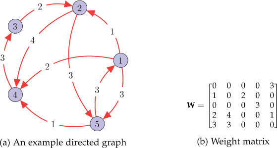
Figure 10.4. Total variation example: a directed graph and its weight matrix

f˜=Wnormf=14.07⎡⎣⎢⎢⎢⎢⎢⎢0102300043020000030030010⎤⎦⎥⎥⎥⎥⎥⎥⎡⎣⎢⎢⎢⎢⎢⎢1031−2⎤⎦⎥⎥⎥⎥⎥⎥=⎡⎣⎢⎢⎢⎢⎢⎢−1.471.720.7400.74⎤⎦⎥⎥⎥⎥⎥⎥, $\tilde{?} = ?^{norm} ? = \frac{1}{4.07} [\begin{matrix} 0 & 0 & 0 & 0 & 3 \\ 1 & 0 & 2 & 0 & 0 \\ 0 & 0 & 0 & 3 & 0 \\ 2 & 4 & 0 & 0 & 1 \\ 3 & 3 & 0 & 0 & 0 \end{matrix}] [\begin{matrix} 1 \\ 0 \\ 3 \\ 1 \\ - 2 \end{matrix}] = [\begin{matrix} - 1.47 \\ 1.72 \\ 0.74 \\ 0 \\ 0.74 \end{matrix}],$

and the total variation of graph signal f with respect to the underlying graph can be calculated as

TVG(f)=||f−f˜||1=10.19. ${T V}_{?} (?) = | | ? - \tilde{?} | |_{1} = 10.19 .$

10.4.4 Graph Fourier Transform

In the Laplacian-based approach, the GFT was defined through the eigendecom-position of the (symmetric) Laplacian matrix. The eigenvalues of the Laplacian matrix were treated as the graph frequencies, and the eigenvectors of the Laplacian were used as the graph Fourier basis. The analogy was derived from the classical Fourier transform through the fact that the complex exponentials act as the eigenfunctions to the 1-D Laplacian operator. Subsequently, the eigenvectors of the Laplacian, or in other words, the eigenfunctions of the graph Laplacian, were treated as the graph Fourier basis. Furthermore, the graph frequencies were ordered based on the quadratic form of the Laplacian, which resulted in a natural frequency order, that is, small eigenvalues as low frequencies, and vice versa. However, in the Laplacian-based approach, the GFT was limited to the undirected graphs with positive edge weights.

In DSP_G, the GFT is defined through the concept of LSI filtering. It makes analogy from the classical Fourier transform from the fact that the classical Fourier bases are invariant to LSI filtering. Thus, to define the GFT, we can use such bases that are invariant to LSI graph filters. From Theorem 10.1, it can be noted that the LSI filters are polynomials in the shift operator, which is the weight matrix of the graph. Therefore, the eigenvectors of the weight matrix of the graph are eigenfunctions of LSI filters and can be used as a graph Fourier basis. Moreover, the corresponding eigenvalues act as graph frequencies.

Assume that the weight matrix of the graph W is diagonalizable.³ Let V=[v0…vN−1]∈CN×N $? = [?_{0} \dots ?_{N - 1}] \in ℂ^{N \times N}$ be the matrix with columns as the eigenvectors of W and Σ∈CN×N $? \in ℂ^{N \times N}$ be the diagonal matrix of corresponding eigenvalues σ₀, σ₁,... , σ_N₋₁ of W. Therefore, the eigendecomposition of W is

(10.4.9) W=VΣV−1. $? = {? ? ?}^{- 1} .$

The graph transform decomposes a graph signal in terms of the graph Fourier basis, that is, the eigenvectors of W. Hence the GFT of a graph signal f is defined as

(10.4.10) fˆ=V−1f. $\hat{?} = ?^{- 1} ? .$

The value fˆ(n) $\hat{f} (n)$ indicates how much frequency content corresponding to frequency σ_n is present in the graph signal f.

The inverse graph Fourier transform (IGFT), which reconstructs the signal back from its graph Fourier transform coefficients, is given by

(10.4.11) f=Vfˆ. $? = ? \hat{?} .$

The GFT defined under DSP_G is an invertible transform, but it does not follow the Parseval’s theorem, which states that the signal energy in the spatial domain is equal to the energy in the frequency domain.

Frequency Ordering

Having defined the GFT, one needs to order the graph frequencies to identify the low and high frequencies of a graph. For this purpose, TV, defined in Section 10.4.3, is utilized. The graph frequencies are ordered based on the TV values of the eigenvectors of W. The eigenvalues corresponding to the eigenvectors with small TV are called low frequencies, and vice versa. Frequency ordering is established by Theorem 10.2.

Theorem 10.2. Let v_i and v_j be the eigenvectors corresponding to two distinct complex eigenvalues σ_i, σ_j ∈ C of the weight matrix W of the graph G. If the eigenvalue σ_i is located closer to the value |σ_max| on the complex frequency plane than the eigenvalue σ_j; that is, if ||σ_max|− σ_i| < ||σ_max|− σ_j|, then the TVs of these eigenvectors with respect to the graph G satisfy

(10.4.12) TVG(vi)<TVG(vj). ${T V}_{?} (?_{i}) < {T V}_{?} (?_{j}) .$

Proof. From Equation 10.4.8, we can write TV_G(v_i) − TV_G (v_j) as follows:

TVG(vi)−TVG(vj)=||vi−Wnormvi||1−||vj−Wnormvj||1=||vi−W|σmax|vi||1−||vj−W|σmax|vj||1=||vi−σi|σmax|vi||1−||vj−σj|σmax|vj||1=|1−σi|σmax||||vi||1−|1−σj|σmax||||vj||1. $\begin{matrix} {T V}_{?} (?_{i}) - {T V}_{?} (?_{j}) & = | | ?_{i} - ?^{norm} ?_{i} | |_{1} - | | ?_{j} - ?^{norm} ?_{j} | |_{1} \\ = | | ?_{i} - \frac{?}{| σ_{m a x} |} ?_{i} | |_{1} - | | ?_{j} - \frac{?}{| σ_{m a x} |} ?_{j} | |_{1} \\ = | | ?_{i} - \frac{σ_{i}}{| σ_{m a x} |} ?_{i} | |_{1} - | | ?_{j} - \frac{σ_{j}}{| σ_{m a x} |} ?_{j} | |_{1} \\ = | 1 - \frac{σ_{i}}{| σ_{m a x} |} | | | ?_{i} | |_{1} - | 1 - \frac{σ_{j}}{| σ_{m a x} |} | | | ?_{j} | |_{1} . \end{matrix}$

For a non-zero matrix W, σ_max ≠ 0. Consider that all the eigenvectors of W have equal ℓ₁-norms. If ||σ_max|− σ_i| < ||σ_max|− σ_j|, then from the above expression it can be concluded that

TV_G (v_i) < TV_G(v_j)

The frequency ordering for weight matrices with complex spectra is visualized in Figure 10.5. In the complex frequency plane, as one moves away from the eigenvalue with maximum absolute value, the eigenvalues correspond to higher frequencies.

Diagrammatic illustration of frequency ordering from low to high frequencies.

The horizontal and vertical axes divide the graph into four quadrants. The horizontal axis has an arrow on the right making it expandable here and is labeled Re. The vertical axis has an arrow on the top making it expandable here and is labeled Im. A thick circle is drawn with the origin as its center. The points where the circle touches the horizontal axis on the left and right are marked negative of the magnitude of omega subscript max, and the magnitude of omega subscript max respectively. Three concentric circles are drawn with a dashed circumference with the magnitude of omega subscript max as their center. The inner two concentric circles have a smaller than the first thick circle, such that they are drawn within the 1st and 4th quadrants alone. The third concentric circle has a radius greater than the first thick circle, and pass through all four quadrants. Only the left halves of these circles are shown. A point on the innermost circle, omega subscript 0 is marked in the 4th quadrant. Likewise, two points on the middle circle labeled omega subscript 1 and omega subscript 2 are marked in the 1st and 4th quadrants, respectively. A point on the outermost circle, omega subscript (N-1) is marked along its circumference in the 3rd quadrant. A leftward arrow in blue is labeled LF at its right end, and HF at its left end. It is marked within the thick circle from the first to the second quadrant, and from within the innermost to beyond the outermost concentric circle.

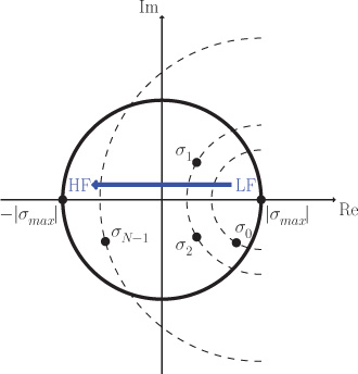
Figure 10.5. Frequency ordering from low frequencies to high frequencies. As one moves away from the eigenvalue with maximum absolute value in the complex frequency plane, the eigenvalues correspond to higher frequencies because the TVs of the corresponding eigenvectors increase.

Example

Consider the directed graph shown in Figure 10.6(a). The eigendecomposition of its weight matrix is W = VΣV⁻¹ , where V and Σ are found to be

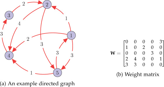
Figure 10.6. A directed graph and its weight matrix

(10.4.13) V=⎡⎣⎢⎢⎢⎢⎢⎢0.360.300.440.590.49−0.560.440.590.27−0.260.26+0.18j−0.21−0.45j0.55−0.28+0.43j0.27+0.11j0.26−0.18j−0.21+0.45j0.55−0.28−0.43j0.27−0.11j−0.750.250.060.050.6⎤⎦⎥⎥⎥⎥⎥⎥ $? = [\begin{matrix} 0.36 & - 0.56 & 0.26 + 0.18 j & 0.26 - 0.18 j & - 0.75 \\ 0.30 & 0.44 & - 0.21 - 0.45 j & - 0.21 + 0.45 j & 0.25 \\ 0.44 & 0.59 & 0.55 & 0.55 & 0.06 \\ 0.59 & 0.27 & - 0.28 + 0.43 j & - 0.28 - 0.43 j & 0.05 \\ 0.49 & - 0.26 & 0.27 + 0.11 j & 0.27 - 0.11 j & 0.6 \end{matrix}]$

(10.4.14) Σ=⎡⎣⎢⎢⎢⎢⎢⎢4.07000001.3900000−1.51+2.35j00000−1.51−2.35j00000−2.44⎤⎦⎥⎥⎥⎥⎥⎥. $? = [\begin{matrix} 4.07 & 0 & 0 & 0 & 0 \\ 0 & 1.39 & 0 & 0 & 0 \\ 0 & 0 & - 1.51 + 2.35 j & 0 & 0 \\ 0 & 0 & 0 & - 1.51 - 2.35 j & 0 \\ 0 & 0 & 0 & 0 & - 2.44 \end{matrix}] .$

Observe the presence of two complex frequencies in the graph spectrum: −1.51 ± 2.35j, where j is the unit imaginary number. From frequency ordering theorem, it is clear that σ_max = 4.07 is the lowest graph frequency, while σ = −2.44 is the highest graph frequency. In the matrix V, the graph Fourier bases are ordered from low to high frequencies where the first column corresponds to the lowest frequency.

Consider a graph signal f = [ 1 0 3 1 −2]^T supported by the graph shown in Figure 10.6(a). Its GFT can be computed as

(10.4.15) fˆ=V−1f=⎡⎣⎢⎢⎢⎢⎢⎢0.752.601.15−0.45j1.15+0.45j−1.93⎤⎦⎥⎥⎥⎥⎥⎥. $\hat{?} = ?^{- 1} ? = [\begin{matrix} 0.75 \\ 2.60 \\ 1.15 - 0.45 j \\ 1.15 + 0.45 j \\ - 1.93 \end{matrix}] .$

Although DSP_G based on a weight matrix is applicable to directed graphs with negative or complex edge weights as well, it does not provide natural intuition of frequency. The eigenvalue with maximum absolute value σ_max acts as the lowest frequency, and as one moves away from this eigenvalue in the complex frequency plane, the frequency increases. Thus, frequency order is not natural and there is an overhead of frequency ordering as well. Also, the interpretation of frequency is not intuitive—for example, in general, a constant graph signal results in lowas well as high-frequency components in the spectral domain.

10.4.5 Frequency Response of LSI Graph Filters

In Section 10.4.2, we discussed LSI graph filters, which are polynomials in the weight matrix W. However, the filters were discussed only in the vertex domain. In this section, frequency domain representation of LSI graph filters is discussed.

From Equations (10.4.4) and (10.4.9), the output of an LSI graph filter H can be written as

(10.4.16) =V[0h(σ0) ⋱h(σN−1)0]V−1fin, $= V [_{0}^{h (σ_{0})} ⋱_{}^{}_{h (σ_{N - 1})}^{0}] V^{- 1} f_{i n},$

where

(10.4.17) h(σℓ)=Σm=0M−1hmσmℓ $h (σ_{ℓ}) = Σ_{m = 0}^{M - 1} h_{m} σ_{ℓ}^{m}$

is known as the frequency response of the filter at frequency σ_ℓ. Given the frequency response of a filter, finding the filter coefficients is a graph filter design problem.

10.5 DSP_G Framework Based on Directed Laplacian

As discussed earlier, selection of a shift operator is key to the DSP_G framework. The directed Laplacian can also be used to derive a shift operator, and as a result, LSI graph filters become polynomials in the directed Laplacian [184]. Subsequently, the directed Laplacian is used as the graph structure matrix whose eigendecomposition is considered as the graph Fourier basis. In contrast to weight matrix–based DSP_G, the difference in frequency ordering and interpretation becomes eventual.

10.5.1 Directed Laplacian

Directed Laplacian is the building block of the DSP_G framework. The definition of graph Laplacian for undirected graphs, which is a difference operator L = D − W, can easily be extended to directed graphs. However, in the case of directed graphs (or digraphs), the weight matrix W of a graph is not symmetric. In addition, the degree of a vertex can be defined in two ways—in-degree and out-degree. In-degree of a node i is estimated as dini=∑Nj=1wij $d_{i}^{i n} = \sum_{j = 1}^{N} w_{i j}$ ; that is, in-degree of a node is the sum of the weights of the incoming edges of the node. On the other hand, out-degree of the node i can be calculated as douti=∑Nj=1wji $d_{i}^{o u t} = \sum_{j = 1}^{N} w_{j i}$ , which is the sum of the weights of the outgoing edges of the node. For node 4 in the directed graph shown in Figure 10.7(a), in-degree is 7 (3 + 2 + 1), whereas, out-degree is 3. Also note that w_ij in the weight matrix of a graph represents the edge weight from node j to node i. In the graph shown in Figure 10.7, the weight of the directed edge from node 1 to node 4 is 2; therefore, w₄₁ = 2.

A directed graph with five nodes is displayed with its weight, in-degree, and Laplacian matrices.

Four figures are present and are labeled alphabetically. Figure a shows the example directed graph which has 5 nodes positioned on the vertices of a pentagon in a counter clockwise manner, such that node 1 is the rightmost node. The following nodes are directed toward the other with the corresponding weights: 1 to 2 with 1, 1 to 3 with 3,1 to 4 with 2, 2 to 4 with 4, 2 to 5 with 3, 3 to 2 with 2, 4 to 3 with 3, 5 to 1 with 3, and 5 and 4 with 1. Figure b shows the Weight matrix W of the graph. The matrix reads the following values row-wise: 0 0 0 0 3, 1 0 2 0 0, 0 0 0 3 0, 2 4 0 0 1, and 3 3 0 0 0. Figure c shows the In-Degree matrix D subscript in of the graph. The matrix reads the following values row-wise: 3 0 0 0 0, 0 3 0 0 0, 0 0 3 0 0, 0 0 0 7 0, and 0 0 0 0 6. Figure d shows the Laplacian matrix L of the graph. The equation is given to be L equals D subscript in minus W. The matrix reads the following values row-wise: 3 0 0 0 -3, -1 3 -2 0 0, 0 0 3 -3 0, -2 -4 0 7 -1, and -3 -3 0 0 6.

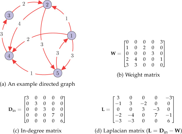
Figure 10.7. A directed graph and the corresponding matrices

The directed Laplacian matrix L of a directed graph is defined as

(10.5.1) L=Din−W, $? = ?_{i n} - ?,$

where Din=diag({dini}Ni=1) $?_{i n} = d i a g ({d_{i}^{i n}}_{i = 1}^{N})$ is the in-degree matrix, which is a diagonal matrix with diagonal entries as the in-degree values of the corresponding nodes. The corresponding matrices of the directed graph of Figure 10.7(a) are shown in Figure 10.7(b–d). Clearly, the Laplacian for a directed graph is not symmetric; nevertheless, it demonstrates some important properties: (i) the sum of each row is zero and hence, λ = 0 is surely an eigenvalue, and (ii) real parts of the eigenvalues are nonnegative for a graph with positive edge weights. These properties of the Laplacian matrix make the frequency analysis of graph signals simple and intuitive.

There also exist a few other definitions of graph Laplacian (normalized as well as combinatorial) for directed graphs. However, selection of the directed Laplacian, as described above, results in a simple and straightforward analysis.

10.5.2 Shift Operator

The directed Laplacian matrix can also be used to derive the shift operator. Similar to the discussion in Section 10.4.1, the shift operator is identified from the graph structure corresponding to a discrete-time periodic signal and then extended to arbitrary graphs.

A finite duration periodic discrete-time signal can be thought of as a graph signal lying on a directed cyclic graph shown in Figure 10.8. Indeed, Figure 10.8 is the support of a periodic time series having a period of five samples. The directed Laplacian matrix of the graph is

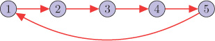
Figure 10.8. A directed cyclic (ring) graph of five nodes. This graph is the underlying structure of a finite duration periodic (with period five) discrete-time signal. All the edges have unit weights.

(10.5.2) L=⎡⎣⎢⎢⎢⎢⎢⎢1−100001−100001−100001−1−10001⎤⎦⎥⎥⎥⎥⎥⎥. $? = [\begin{matrix} 1 & 0 & 0 & 0 & - 1 \\ - 1 & 1 & 0 & 0 & 0 \\ 0 & - 1 & 1 & 0 & 0 \\ 0 & 0 & - 1 & 1 & 0 \\ 0 & 0 & 0 & - 1 & 1 \end{matrix}] .$

Consider a discrete-time finite duration periodic signal x = [ 9 7 1 0 6]^T defined on the graph shown in Figure 10.8. Shifting the signal x by one unit to the right results in the signal x˜=[69710]T $\tilde{?} = [6 9 7 1 0]^{T}$ . This shifted version of the signal can also be found as

where S = (I − L) is treated as the shift operator (matrix).

This notion of shift can be extended to arbitrary graphs and consequently can be used S = (I − L) as the shift operator for graph signals. Hence, the shifted version of a graph signal f can be calculated as

(10.5.3) f˜=Sf=(I−L)f. $\tilde{?} = ? ? = (? - ?) ? .$

Recall that shift operation can also be achieved by using the weight matrix (Section 10.4). However, selecting S = (I − L) as the shift operator results in a better and simpler frequency analysis of graph signals, which will become evident in the following sections.

10.5.3 Linear Shift Invariant Graph Filters

It was proved in the previous section that when weight matrix W is chosen as the shift operator, LSI graph filters are polynomials in W. However, when I − L is chosen as the shift operator, an LSI graph filter turns out to be a polynomial in the directed Laplacian L instead of W. It is proved by Theorem 10.3.

Theorem 10.3. A graph filter H is LSI if the following conditions are satisfied:

1. Geometric multiplicity of each distinct eigenvalue of the graph Laplacian is one.

2. The graph filter H is a polynomial in L; that is, H can be written as

(10.5.4) H=h(L)=Σm=0M−1hmLm=h0I+h1L+…+hM−1LM−1, $H = h (L) = Σ_{m = 0}^{M - 1} h_{m} L^{m} = h_{0} I + h_{1} L + \dots + h_{M - 1} L^{M - 1},$

where h0,h1,…,hM−1∈C $h_{0}, h_{1}, \dots, h_{M - 1} \in ℂ$ are called filter taps.

Proof. From Equation (10.5.3), the shift operator is S = I − L. Then, for a filter H to be LSI, the following must be satisfied:

S(Hf)or,(I−L)(Hf)or,LH=H(Sf)=H((I−L)f)=HL. $\begin{matrix} ? (? ?) & = ? (? ?) \\ o r, (? - ?) (? ?) & = ? ((? - ?) ?) \\ o r, ? ? & = ? ? . \end{matrix}$

In other words, the filter is LSI if the matrices L and H commute. This is true when H is a polynomial in L, given that the characteristic polynomial and the minimal polynomial of L are equal or the geometric multiplicity of every distinct eigenvalue is one.^a

a. The characteristic polynomial and the minimal polynomial of a matrix are equal if the dimension of eigenspace associated with every eigenvalue is one. Equivalently, it holds if there is a unique Jordan block associated with each eigenvalue.

Considering a 2-tap graph filter and substituting h₀ = 1 and h₁ = −1 in Equation (10.5.4), we get H = S = I − L, which is the shift operator discussed in Section 10.5.2. Thus, the shift operator is a first-order LSI filter. Also, the graph Fourier bases, which are the Jordan eigenvectors of L, are the eigenfunctions of an LSI filter described by Equation (10.5.4).

10.5.4 Total Variation

As discussed earlier, the TV of a graph signal is a measure of total amplitude oscillations in the signal values with respect to the graph. For time series and image signals, TV is defined as ℓ₁-norm of the signal derivative. This definition is extended to graph settings, and subsequently, the TV of a graph signal f with respect to the graph G $?$ can be given as

(10.5.5) TVG(f)=Σi=1N|∇i(f)|, ${T V}_{?} (f) = Σ_{i = 1}^{N} | \nabla_{i} (f) |,$

(10.5.6) ∇i(f)=(f−f˜)(i). $\nabla_{i} (?) = (? - \tilde{?}) (i) .$

From Equation (10.5.3), (10.5.5), and (10.5.6), we have

(10.5.7) TVG(f)=Σi=1N|f(i)−f˜(i)|=||f−f˜||1=||Lf||1. ${T V}_{?} (f) = Σ_{i = 1}^{N} | f (i) - \tilde{f} (i) | = | | f - \tilde{f} | |_{1} = | | L f | |_{1} .$

Observe that the quantity Lf at node i is the sum of the weighted differences (weighted by corresponding edge weights) between the value of f at node i and values at the neighboring nodes. In other words, (Lf)(i) = ∇_i(f) provides a measure of variations in the signal values as one moves from node i to its adjacent nodes. Thus, ℓ₁-norm of the quantity Lf can be interpreted as the absolute sum of the local variations in f. This definition of TV is intuitive, as opposed to the one defined in DSP_G which results in a non-zero TV value for a constant graph signal. TV given by Equation (10.5.7) will be utilized to estimate variations of the graph Fourier basis and subsequently to identify low and high frequencies of a graph.

10.5.5 Graph Fourier Transform Based on Directed Laplacian

Fourier-like analysis of graph signals provides a means to analyze structured data in the frequency (spectral) domain. In the classical Fourier transform, the complex exponentials are treated as the Fourier basis. The existing Laplacian-based method defines the GFT by making analogy from the classical Fourier transform in a sense that the complex exponentials are the eigenfunctions of the 1-D Laplace operator. Therefore, analogously, the eigenvectors of the graph Laplacian (symmetric) are used as the graph harmonics. On the other hand, DSP_G derives analogy from the perspective of LSI filtering. In DSP_G, LSI graph filters are polynomials in the graph weight matrix W, and as a result, the eigenvectors of W become the eigenfunctions of LSI graph filters. Analogous to the fact that the complex exponentials are invariant to LSI filtering in classical signal processing, the eigenvectors of W are utilized as the graph Fourier bases.

As discussed earlier, DSP_G derives analogy from the perspective of LSI filtering in the sense that complex exponentials (classical Fourier basis) are eigenfunctions of linear time invariant (LTI) filters. Now that LSI graph filters are polynomials in the directed Laplacian matrix L (Theorem 10.3), the eigenvectors of L can be used as graph Fourier bases because they are eigenfunctions of LSI graph filters. Using Jordan decomposition, the graph Laplacian is decomposed as

(10.5.8) L=VJV−1, $? = {? ? ?}^{- 1},$

where J, known as the Jordan matrix, is a block diagonal matrix similar to L and the Jordan eigenvectors of L constitute the columns of V. Now, GFT of a graph signal f can be defined as

(10.5.9) fˆ=V−1f. $\hat{?} = ?^{- 1} ? .$

Here, V is treated as the graph Fourier matrix whose columns constitute the graph Fourier basis. IGFT can be calculated as

(10.5.10) f=Vfˆ. $? = ? \hat{?} .$

In this definition of GFT, the eigenvalues of the graph Laplacian act as the graph frequencies and the corresponding Jordan eigenvectors act as the graph harmonics. The eigenvalues with small absolute value correspond to low frequencies, and vice versa. Proof of this is provided later in this section (see Theorem 10.4). Thus, the frequency order turns out to be natural.

Now, we discuss two special cases: (i) when the directed Laplacian matrix is diagonalizable and (ii) undirected graphs.

Diagonalizable Laplacian Matrix

When the directed Laplacian is diagonalizable, Equation (10.5.8) is reduced to

(10.5.11) L=VΛV−1. $? = ? ? ?^{- 1} .$

Here, Λ∈CN×N $? \in ℂ^{N \times N}$ is a diagonal matrix containing the eigenvalues λ₀, λ₁,... , λ_N₋₁ of L and V=[v0,v1,…,vN−1]∈CN×N $? = [?_{0}, ?_{1}, \dots, ?_{? - 1}] \in ℂ^{N \times N}$ is the matrix with columns as the corresponding eigenvectors of L. Note that for a graph with real nonnegative edge weights, the graph spectrum lies in the right half of the complex frequency plane (including the imaginary axis).

Undirected Graphs

For an undirected graph with real weights, the directed Laplacian matrix L is real and symmetric. As a result, the eigenvalues of L turn out to be real and L constitutes an orthonormal set of eigenvectors. Hence, the Jordan form of the Laplacian matrix for undirected graphs can be written as

(10.5.12) L=VΛVT, $? = ? ? ?^{T},$

where V^T = V⁻¹ , because the eigenvectors of L are orthogonal in the undirected case. Consequently, the GFT of a signal f can be given as fˆ=VTf $\hat{?} = ?^{T} ?$ and the inverse can be calculated as f=Vfˆ $? = ? \hat{?}$ . Note that the graph spectrum lies on the real axis of the complex frequency plane, given the weight matrix is real. Moreover, if the weights are real and nonnegative, the graph spectrum lies on the nonnegative half of the real axis. This case is equivalent to the definition of GFT based on (symmetric) Laplacian, where only undirected graphs with real and nonnegative weights were considered. Thus, the definition of GFT based on directed Laplacian unifies DSP_G and (symmetric) Laplacian-based approach.

Frequency Ordering

Having defined the GFT based on directed Laplacian, one needs to identify which eigenvalues correspond to low or high frequencies. The definition of TV given by Equation (10.5.7) is utilized to quantify oscillations in the graph harmonics and subsequently to order the frequencies. Analogous to classical signal processing, the eigenvalues are labeled as low frequencies for which the corresponding proper eigenvectors have small variations, and vice versa. The frequency ordering is established by Theorem 10.4.

Theorem 10.4. Let v_i and v_j be the eigenvectors corresponding to two distinct complex eigenvalues λi,λj∈C $λ_{i}, λ_{j} \in ℂ$ of the Laplacian matrix L of the graph G $?$ . If |λ_i| > |λ_j|, then the TVs of these eigenvectors with respect to the graph G $?$ satisfy

(10.5.13) TVG(vi)>TVG(vj). ${T V}_{?} (?_{i}) > {T V}_{?} (?_{j}) .$

Proof. Let v_r be the proper eigenvector corresponding to eigenvalue λ_r of the Laplacian matrix L of the graph G $?$ , then Lv_r = λ_rv_r. Now, using Equation (10.5.7), the TV of v_r with respect to the graph G $?$ is calculated as

TVG(vr)=||Lvr||1=||λrvr||1=|λr|(||vr||1). ${T V}_{?} (?_{r}) = | | {? ?}_{r} | |_{1} = | | λ_{r} ?_{r} | |_{1} = | λ_{r} | (| | ?_{r} | |_{1}) .$

If all the eigenvectors scaled to have the same ℓ₁-norm, then from the above analysis it can be noted that

(10.5.14) TVG(vr)∝|λr|. ${T V}_{?} (?_{r}) \propto | λ_{r} | .$

Figure 10.9 shows the visualization of frequency ordering in the complex frequency plane, where λ₀ = 0 corresponds to zero frequency and, as one moves away from the origin, the eigenvalues correspond to higher frequencies. Note that the TV of a proper eigenvector is directly proportional to the absolute value of the corresponding eigenvalue. Therefore, all the proper eigenvectors corresponding to the eigenvalues having equal absolute value will have the same TV. For example, in Figure 10.9(a) and (b), the TV values of eigenvectors corresponding to eigenvalues λ₁, λ₂, and λ₃ are equal. As a result, distinct eigenvalues may sometimes yield exactly same TV. For this reason, sometimes frequency ordering is not unique. However, if all the eigenvalues are real, the frequency ordering is guaranteed to be unique. Figure 10.9(c) shows the ordering in the case of an undirected graph with real edge weights. In this case, the directed Laplacian is symmetric and, therefore, the graph frequencies are real. Moreover, if an undirected graph has real and nonnegative edge weights, the directed Laplacian will be a symmetric and positive semidefinite matrix. Frequency ordering visualization for this case is shown in Figure 10.9(d).

A four-part illustration of frequency ordering from low to high frequencies.

The illustration is divided into four parts that are labeled alphabetically and placed two in a row. Figure a shows the ordering for a graph with positive or negative edge weights. The horizontal and vertical axes divide the graph into four quadrants. The horizontal axis has an arrow on the right making it expandable here and is labeled Re. The vertical axis has an arrow on the top making it expandable here and is labeled Im. Three concentric circles are drawn with a dashed circumference and with the origin as their center. The difference in radii between the inner two circles is much lesser when compared to the radii difference between the middle and outer circles. The Re axis between the outer two circles are is shown dotted on both positive and negative sides, denoting that the axis is expendable here. The origin is marked lambda subscript 0. The point where the second circle touches the positive of the Re axis is lambda subscript 1. Two points on the middle circle in the second and third quadrants are labeled lambda subscript 2 and lambda subscript 3, respectively. Similarly, two points on the outermost circle in the first and fourth quadrants are labeled lambda subscript (N-1) and lambda subscript (N-2), respectively. Two blue arrows point from the origin to the top-left and right respectively, such that the arrows are inclined at an angle of 120 degrees, approximately. The pointed ends of the arrows are labeled HF, while the other end is labeled LF. Figure b shows the ordering for a graph with positive edge weights. The right half comprising of the first and fourth quadrants from the figure a is shown here. Lambda subscript 2 and lambda subscript 3 that were along the middle circle in the 2nd and 3rd quadrants are mapped onto the 1st and 4th respectively. Figure c shows the ordering for an undirected graph with real edge weights. Here the Re and Im axis are retained, and the following are marked along the Re axis from the left: lambda subscript (N-1), lambda subscript 1, lambda subscript 0 at the origin, and lambda subscript (N-2). The Re axis is shown dotted on both positive and negative sides before the lambda subscript (N-1) and lambda subscript (N-2), denoting that the axis is expendable here. Two blue arrows point from the origin to the left and right respectively, such that the arrows are inclined at an angle of 180 degrees. The pointed ends of the arrows are labeled HF, while the other end is labeled LF. Figure d shows the ordering for an undirected graph with real and nonnegative edge weights. The right half comprising of the positive Re axis from the figure c is shown here. Lambda subscript 1 and lambda subscript (N-1) are mapped onto the positive Re axis.

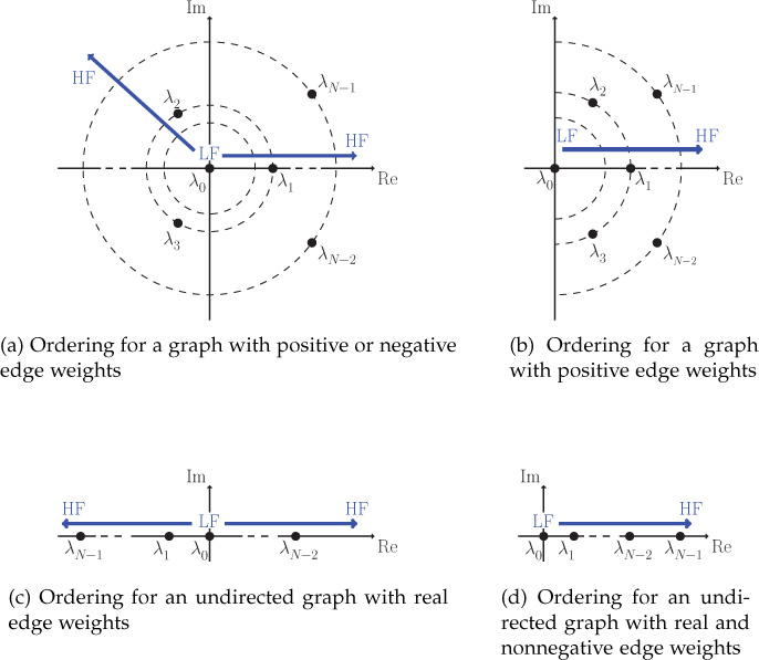
Figure 10.9. Frequency ordering from low frequencies to high frequencies. As one moves away from the origin (zero frequency) in the complex frequency plane, the eigenvalues correspond to higher frequencies because the TVs of the corresponding eigenvectors increase.

Example

Let us consider a directed graph, shown in Figure 10.10(a). Performing Jordan decomposition of the Laplacian matrix, the Fourier matrix V and Jordan matrix J are as follows:

A directed graph with five nodes is displayed with its Laplacian matrix.

Figure 10.10. A directed graph and its directed Laplacian matrix

V=⎡⎣⎢⎢⎢⎢⎢⎢0.4470.4470.4470.4470.4470.680−0.502−0.502−0.1080.146−0.232−0.134j0.232+0.312j−0.502−0.201j0.618−0.089j0.309−0.232+0.134j0.232−0.312j−0.502+0.201j0.618+0.089j0.309−0.5350.0800.080−0.1250.828⎤⎦⎥⎥⎥⎥⎥⎥ $? = [\begin{matrix} 0.447 & 0.680 & - 0.232 - 0.134 j & - 0.232 + 0.134 j & - 0.535 \\ 0.447 & - 0.502 & 0.232 + 0.312 j & 0.232 - 0.312 j & 0.080 \\ 0.447 & - 0.502 & - 0.502 - 0.201 j & - 0.502 + 0.201 j & 0.080 \\ 0.447 & - 0.108 & 0.618 - 0.089 j & 0.618 + 0.089 j & - 0.125 \\ 0.447 & 0.146 & 0.309 & 0.309 & 0.828 \end{matrix}]$

J=⎡⎣⎢⎢⎢⎢⎢⎢0000002.354000006.000−1.732j000006.000+1.732j000007.646⎤⎦⎥⎥⎥⎥⎥⎥ $? = [\begin{matrix} 0 & 0 & 0 & 0 & 0 \\ 0 & 2.354 & 0 & 0 & 0 \\ 0 & 0 & 6.000 - 1.732 j & 0 & 0 \\ 0 & 0 & 0 & 6.000 + 1.732 j & 0 \\ 0 & 0 & 0 & 0 & 7.646 \end{matrix}]$

The diagonal entries in J are the eigenvalues of the Laplacian matrix and constitute the graph spectrum. Eigenvalue λ = 7.646 corresponds to the highest frequency of the graph. Also note that the TVs of the eigenvectors corresponding to the frequencies λ = 6 − 1.732j and λ = 6 + 1.732j are equal because both the frequencies have the same absolute value. The magnitudes of the GFT coefficients of the graph signal f = [ 0.12 0.38 0.81 0.24 0.88]^T are plotted in Figure 10.11.

The magnitude spectrum of a graph signal for a weighted graph with five nodes is displayed.

The 3D axes are marked with Re (lambda subscript l), Im (lambda subscript l), and the magnitude of f circumflex (lambda subscript l), respectively. Planes are extended from each of the axes, with girds on them according to the grading along each axis, such that the graph appears to be a room with three walls. The Re axis is marked with values from 0 to 8 in increments of 2, the Im axis is marked from -10 to 10 in increments of 5, and the other vertical axis is marked with values from 0 to 1.5 in increments of 0.5. The graph is drawn on the plane that forms the floor of the room. Three curves are drawn along this plane with the following Re-Im coordinates. The first curve begins at (0, -7), reaches a peak at (7.8, 0), and ends at (0, 7). The second curve begins at (0, -6), reaches a peak at (6, 0), and ends at (0, 6). The third curve, which is the innermost curve begins at (0, -3), reaches a peak at (2, 0), and ends at (0, 3). The curves are drawn in red, and the area enclosed by them on the plane is shaded green. A thick line is drawn from (0, 0) to (6.8, 0), bisecting the three curves. From the following points along the curves blue pins are extended up with respect to all three axes: (6.8, 0, 0) to (6.8, 0, 0.6), (6, -5, 0) to (6, -5, 0.4), (6, 5, 0) to (6, 5, 0.4), (2, 0, 0) to (2, 0, 0.2), and (1, 3, 0) to (1, 3, 0.5). The coordinate values are only approximate.

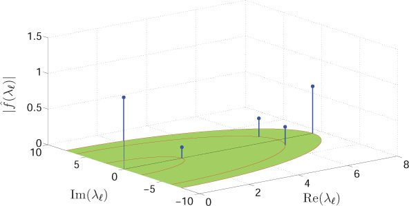
Figure 10.11. Magnitude spectrum of the graph signal f = [ 0.12 0.38 0.81 0.24 0.88]^T defined on the graph shown in Figure 10.10(a)

Concept of Zero Frequency

The Jordan eigenvector corresponding to the zero eigenvalue is given as v0=1N√[11…1]T $?_{0} = \frac{1}{\sqrt{N}} [1 1 \dots 1]^{T}$ . Therefore, for a constant graph signal, the GFT will have only a single non-zero coefficient at zero frequency (eigenvalue). For example, consider a constant graph signal f = [ 1 1 1 1 1]^T residing on the graph shown in Figure 10.10(a). The GFT of the signal is fˆ=[5–√0000]T $\hat{?} = [\sqrt{5} 0 0 0 0]^{T}$ , magnitudes of which are plotted in Figure 10.12.

The magnitude spectrum of a constant signal for a weighted graph with five nodes is displayed.

The 3D axes are marked with Re (lambda subscript l), Im (lambda subscript l), and the magnitude of f circumflex (lambda subscript l), respectively. Planes are extended from each of the axes, with girds on them according to the grading along each axis, such that the graph appears to be a room with three walls. The Re axis is marked with values from 0 to 8 in increments of 2, the Im axis is marked from -10 to 10 in increments of 5, and the other vertical axis is marked with values from 0 to 3 in unit increments. The graph is drawn on the plane that forms the floor of the room. Three curves are drawn along this plane with the following Re-Im coordinates. The first curve begins at (0, -7), reaches a peak at (7.8, 0), and ends at (0, 7). The second curve begins at (0, -6), reaches a peak at (6, 0), and ends at (0, 6). The third curve, which is the innermost curve begins at (0, -3), reaches a peak at (2, 0), and ends at (0, 3). The curves are drawn in red, and the area enclosed by them on the plane is shaded green. A thick line is drawn from (0, 0) to (6.8, 0), bisecting the three curves. The following points are marked in blue, along the curves with respect to the Re-Im axes: (6.8, 0), (6, -5), (6, 5), and (2, 0). From the point (0, 0, 0) a blue pin is extended up to the point (0, 0, 1.2). The coordinate values are only approximate.

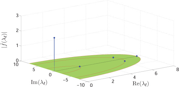
Figure 10.12. Magnitude spectrum of a constant signal f = [ 1 1 1 1 1]^T defined on the graph shown in Figure 10.10(a)

One can observe the presence of only a zero frequency component in the spectrum of a constant graph signal. This is in agreement with the intuition that the variation in a constant graph signal is zero as one travels from one node to another node connected by a directed edge. In contrast, the GFT defined in DSP_G fails to give this basic intuition.

An important point worth mentioning here is that same order of frequency can be achieved, as given by Theorem 10.4, even if quadratic form (2-Dirichlet form) is used in place of TV. p-Dirichlet form of a signal f is defined as

(10.5.15) Sp(f)=1pΣi=1N|∇i(f)|p. $S_{p} (f) = \frac{1}{p} Σ_{i = 1}^{N} | \nabla_{i} (f) |^{p} .$

Putting p = 2 in the above equation, we get 2-Dirichlet form:

(10.5.16) S2(f)=12∑i=1N|∇i(f)|2. $S_{2} (?) = \frac{1}{2} \sum_{i = 1}^{N} | \nabla_{i} (?) |^{2} .$

Substituting ∇_i(f) from Equation (10.5.6), we have

(10.5.17) S2(f)=12Σi=1N|f(i)−f˜(i)|2=12||f−f˜||22=12||Lf||22. $S_{2} (f) = \frac{1}{2} Σ_{i = 1}^{N} | f (i) - \tilde{f} (i) |^{2} = \frac{1}{2} | | f - \tilde{f} | |_{2}^{2} = \frac{1}{2} | | L f | |_{2}^{2} .$

Now, using the above equation, quadratic form of a proper eigenvector v_r corresponding to frequency λ_r can be calculated as S2(vr)=12||Lvr||22=12||λrvr||22=12|λr|2||vr||22 $S_{2} (?_{r}) = \frac{1}{2} | | {? ?}_{r} | |_{2}^{2} = \frac{1}{2} | | λ_{r} ?_{r} | |_{2}^{2} = \frac{1}{2} | λ_{r} |^{2} | | ?_{r} | |_{2}^{2}$ . Therefore, if all the eigenvectors are scaled to have the same ℓ₂-norm, then

(10.5.18) S2(vr)∝|λr|2. $S_{2} (?_{r}) \propto | λ_{r} |^{2} .$

In other words, 2-Dirichlet form of a graph harmonic is proportional to the square of the corresponding frequency amplitude, and hence, the frequency ordering based on the quadratic form will be same as given by Theorem 10.4.

From the above discussion, it can be argued that GFT based on directed Laplacian provides natural intuition of frequency. Therefore, it allows extension of SGWT to directed graphs. SGWT is discussed in Chapter 11.

10.5.6 Frequency Response of LSI Graph Filters

Filtering can be characterized in the frequency domain using GFT. Assume that L is diagonalizable as in Equation (10.5.11). From Equation (10.5.4), the output f_out of an LSI graph filter to an input graph signal f_in is

(10.5.19) fout=h(L)fin=h(VΛV−1)fin=Vh(Λ)V−1fin, $?_{o u t} = h (?) ?_{i n} = h (? ? ?^{- 1}) ?_{i n} = ? h (?) ?^{- 1} ?_{i n},$

where h(Λ)=diag{h(λ0),h(λ1),…,h(λN−1)} $h (?) = d i a g {h (λ_{0}), h (λ_{1}), \dots, h (λ_{N - 1})}$ with h(λℓ)=∑M−1m=0hmλmℓ $h (λ_{ℓ}) = \sum_{m = 0}^{M - 1} h_{m} λ_{ℓ}^{m}$ . Now, from the definition of GFT and Equation (10.5.19), it follows that

(10.5.20) fˆout=h(Λ)fˆin. ${\hat{?}}_{o u t} = h (?) {\hat{?}}_{i n} .$

To put Equation (10.5.20) in other words, the filter output in the frequency domain is equivalent to the element-wise multiplication of the input signal spectrum and the diagonal entries of h(Λ). Here, h(Λ) is known as the frequency response of the LSI graph filter. This multiplication in the graph spectral domain is a generalization of the classical convolution theorem⁴ to graph settings.

10.6 Comparison of Graph Signal Processing Approaches

Table 10.1 compares various features of the two approaches of GSP. The Laplacian-based approach is limited to undirected graphs, whereas DSP_G is applicable to directed graphs. Moreover, DSP_G provides the theory of LSI similar to the one existing in classical signal processing. The key to the DSP_G frameworks is the shift operator. Depending on the choice of the shift operator, the structure matrix of the graph is either the weight matrix or the directed Laplacian matrix. Frequency interpretation and ordering is natural if a directed Laplacian matrix is used as the graph representation matrix under the DSP_G framework.

Table 10.1. Comparison of the graph signal processing frameworks

	GSP Based on Laplacian	DSP_G Framework
	GSP Based on Laplacian	Based on Weight Matrix	Based on Directed Laplacian
Applicability	Undirected graphs	Directed as well as undirected graphs	Directed as well as undirected graphs
Frequencies	Eigenvalues of the Laplacian matrix (real)	Eigenvalues of the weight matrix (complex)	Eigenvalues of the directed Laplacian matrix (complex)
Harmonics	Eigenvectors of the Laplacian matrix (real)	Jordan eigenvectors of the weight matrix (complex)	Jordan eigenvectors of the directed Laplacian matrix (complex)
Frequency Ordering	Laplacian quadratic form (natural)	Total variation (not natural)	Total variation (natural)
Shift Operator	Not defined	The weight matrix W	Derived from the directed Laplacian matrix (I − L)
LSI Filters	Not applicable	Applicable	Applicable

10.7 Open Research Issues

Designing dictionaries for sparsely represented graph signals is an active area of research. Dictionary learning has been widely studied in image processing, computer vision, and machine learning. The task of dictionary learning is to find a sparse representation of the training data as a linear combination of basic building blocks or atoms. In graph settings, the challenges in dictionary learning are that the dictionary should have the ability to adapt to specific signal data, it should be implementable in a computationally efficient manner, and it should incorporate the irregular graph structure into the atoms of the dictionary. Some efforts in this direction can be found in [185][186].
The Fourier transforms defined in all the above discussed approaches require full eigendecomposition of the weight matrix or the directed Laplacian matrix, computation of which is extremely costly. Development of fast algorithms for computing the transforms will help faster and efficient computation of the transforms. Some recent efforts made in this direction can be found in [171] and [172].
The eigendecomposition of the weight matrix or the directed Laplacian matrix does not form an orthogonal basis and, therefore, the signal energy is not preserved in the graph Fourier domain. Developement of orthogonal graph Fourier basis for directed graphs is an interesting area to explore. Recent efforts in this direction can be found in [187] and [188].
Development of various techniques for designing graph filters is an active area of research. The task of graph filter design is to find the coefficinets of matrix polynomials to acheive the desired graph frequency response. However, perfect implementation is not always possible. Designing more and more accurate graph filters is an open problem. Works in this direction include [189], [176], and [190].
Deriving new shift operators that are closer to the classical shift is an interesting field of research. In [191], authors proposed a set shift operators that satisfy the energy conservation property similar to its counterpart in classical signal processing. Problem 20 in the end-of-chapter exercises is based on their proposed shift operator. Moreover, in [192], the authors introduce an isometric shift operator, a matrix whose eigenvalues are derived from the graph Laplacian matrix, that also satisfies the energy conservation property.
Different approaches for sampling theory for graph signals have been proposed in [164], [173], [174], and [175]. However, the area is open for development of a simple and generalized sampling theory for data defined on complex networks.
Development of multirate signal processing tools such as filter banks and wavelets under the DSP_G framework is an active area of research. Perfect reconstruction two-channel wavelet filter banks were developed in [193]. However, this approach is based on undirected graph Laplacian and is limited to undirected graphs. Some recent efforts in the direction of development of M-channel filter banks can be found in [194] and [195].
The directed Laplacian used in the existing theory is derived from the in-degree matrix. However, the directed Laplacian can also be defined as L = D_out − W, and based on that, an equivalent theory can be developed.
Data generated by complex networks is very huge. Techniques for compression of data lying on such huge graphs is an open area of research. Also, development of application-specific transforms is an active area.

10.8 Summary

This chapter presented existing approaches for graph signal processing: (1) the Laplacian-based approach and (2) the DSP_G framework. The Laplacian-based framework is limited to undirected graphs with only positive edge weights. On the other hand, DSP_G is applicable to directed graphs with complex edge weights as well. The DSP_G framework relies on a shift operator based on which concepts, such as shift invariance, total variation, and GFT, are defined. Two popular choices of the shift operator, derived from the weight matrix and the directed Laplacian, were presented. Based on these shift operators, the DSP_G framework was discussed in detail. However, one can derive other suitable shift operators and accordingly choose graph structure matrices.

Exercises

Consider the graph G $?$ shown in Figure 10.13.

A directed graph G with five nodes is displayed.

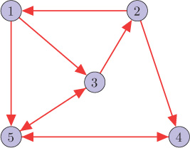
Figure 10.13. Graph G $?$

1. For the graph G $?$ shown in Figure 10.13, compute the following using the weight matrix–based approach:

(a) Shifted version of a graph signal f = [ 2, −3, 1, 8, 0]^T.

(b) Total variations of all the eigenvectors.

2. Considering eigenvalues of weight matrix as graph frequencies, order the following eigenvalues from low to high frequencies.

(a) 1.0264, 3.5663, −2.3504, −1.4289, −0.8134

(b) 0, 0.1668, −1.4685 − 0.0883j, −1.4685 + 0.0883j, 2.7703

Also comment on the directivity and nature of edge weight (positive, real, or complex) of the graphs.

3. Consider a five-node directed ring graph, as shown in Figure 10.14. Identify a matrix operator using (a) the weight matrix, (b) the in-degree directed Laplacian, and (c) the out-degree directed Laplacian of the graph that shifts a signal one step left. That is, for a signal [ 1, 2, 3, 4, 5]^T, the shifted version should be [ 2, 3, 4, 5, 1]^T.

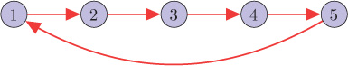
A string network is shown. It has six nodes, numbered as such and connected along a horizontal line. Every node points to the next node. Node 5 points back to node 1.

Figure 10.14. A directed ring graph with five nodes

4. Repeat the Problem 1 using the directed Laplacian-based approach.

5. Repeat Problem 2 if the given eigenvalues are of the directed Laplacian matrix.

6. The oscillations in a signal lying on a network can also be quantified by the number of zero crossings in the signal values. If there is a directed edge from node i to node j and there is a change in the sign of the signal values at nodes i and j, then it is counted as one zero crossing. Create a directed random network with 300 nodes by adding a directed edge between any two nodes with a probability of 0.15.

(a) Plot the number of zero crossings separately in real and imaginary parts of the eigenvectors of the in-degree Laplacian matrix with respect to the magnitudes of the corresponding eigenvalues. Comment on your observations and explain the frequency ordering.

(b) Repeat part (a) for the weight matrix of the network.

7. Derive a shift operator by using the normalized weight matrix P = D⁻¹/2WD⁻¹/2 of a graph (analogy can be made from the case of discrete-time signals). Subsequently, redefine total variation and GFT.

8. For a graph signal lying on an N-node directed ring graph, considering the weight matrix as the shift operator, answer the following:

(a) Write down the TV expression for the graph Fourier basis.

(b) Identify and order the graph frequencies.

9. Prove that the GFT associated with a Cartesian product graph is given by the matrix Kronecker product of the GFTs for its factor graphs (use weight matrix as shift operator). Also comment on the spectrum of the Cartesian product graph.

Verify your results for the Cartesian product of the two graphs given in Figure 10.15. You can choose any values for the signals defined on the graphs.

Two connected graphs are placed side-by-side.

Figure 10.15. Graphs for Problem 9

Hint: Refer to Section 2.5.9 for the definitions of product graphs.

10. Consider a graph signal f = [ 3, − 2, 0, 1, 6]^T defined on the graph shown in Figure 10.13. Compute the outputs f₁ and f₂ of LSI graph filters in cascade, as shown in Figure 10.16, for the following cases:

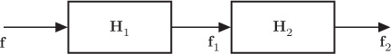
Figure 10.16. Filters in cascade (Problem 10)

(a) H₁ = 3I − 2W + W² and H₂ = I + 4W.

(b) H₁ = 3I − 2L + L² and H₂ = I + 4L.

Use the vertex domain as well as the frequency domain methods to find the output graph signals and verify your results. Also, draw frequency responses of the filters. Can you find an equivalent filter H for the two filters H₁ and H₂ in cascade?

11. This problem is about designing LSI graph filters using least squares. An LSI graph filter can be defined through its frequency response h(σ_ℓ) at its distinct frequencies σ_ℓ , for ℓ = 0, 1, . . . , N − 1. In the weight matrix based DSP_G framework, an LSI graph filter is a polynomial (in the weight matrix) of degree M. To construct an LSI filter with frequency response h(σ_ℓ) = b_ℓ , one need to solve a system of N linear equations with M + 1 unknowns h₀, h₁,... , h_M:

(10.8.1) h0+h1σ0+…+hLσM0h0+h1σ1+…+hLσM1h0+h1σN−1+…+hLσMN−1=b0,=b1,⋮=bN−1. $\begin{matrix} h_{0} + h_{1} σ_{0} + \dots + h_{L} σ_{0}^{M} & = b_{0}, \\ h_{0} + h_{1} σ_{1} + \dots + h_{L} σ_{1}^{M} & = b_{1}, \\ ⋮ \\ h_{0} + h_{1} σ_{N - 1} + \dots + h_{L} σ_{N - 1}^{M} & = b_{N - 1} . \end{matrix}$

In general, N > M + 1, and therefore, the system of linear equations is overdetermined and does not have a solution. In this case, an approximate solution can be found in the least-squares sense.

Design the filters with the following specifications using least squares for the graph shown in Figure 10.17.

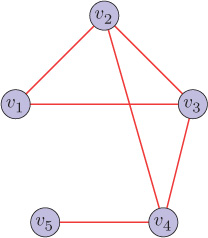
A connected graph with five nodes is displayed.

Figure 10.17. Graph for Problem 11

(a) A low-pass filter of order two that passes only the smallest two frequencies.

(b) A high-pass filter of order two that passes only the largest two frequencies.

12. This problem illustrates utilization of GFT in sensor malfunction detection. You will first create anomalous data and then validate the anomaly in the data by utilizing GFT. Using GSPBox (see Appendix G for additional information on GSPBox), create a 50-node random sensor network and define a signal f on the graph as

(10.8.2) f(i)={1010e−c.d(i,30)ifi=30otherwise, $? (i) = {\begin{matrix} 10 & if i = 30 \\ 10 e^{- c . d (i, 30)} & otherwise, \end{matrix}$

where c is a constant and d(i, j) is the distance between nodes i and j (can be found using Dijkstra’s shortest path algorithm). This signal can be thought of as temperature values in a geographical area, since the variations in temperature values are not high if the sensors are placed densely.

(a) Plot the graph signal and its spectrum for c = 0.1. Now assume that sensors 31 and 42 are anomalous and show temperature values of zero.

(b) Plot the spectrum of this anomalous data. Can we conclude that the data generated by the sensor network is anomalous?

13. (a) Prove that the operator L^K is localized within K hops at each node, that is, (L^K)_ij = 0 for d_G(i, j) > K, where L is the directed Laplacian matrix (in-degree) of a graph G $?$ and d_{G $?$}(i, j) is the hop distance from node j to node i. In other words, to compute L^Kf at node i, we need the signal values only at the nodes from which node i can be reached within K hops. Consequently, show that a polynomial of order K in the directed Laplacian matrix L is also localized within K hops at each node.

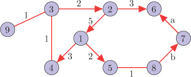
(b) A signal f = [ 3, 0, 2, 4, 0, 1, 2, 3, 5]^T is defined on the graph G $?$ as shown in Figure 10.18. The edge weights a and b are unknown. Consider two polynomial filters

A graph weighted G with nine nodes is displayed.

Figure 10.18. Graph G $?$ for Problem 13

(10.8.3) H1=3I−2L $?_{1} = 3 ? - 2 ?$

and

(10.8.4) H2=I+3L−L2, $?_{2} = ? + 3 ? - ?^{2},$

where L is the directed Laplacian matrix (in-degree).

(i) What is the sum of the elements of each row of H₁ and H₂?

(ii) For filter H₁, compute the filtered output at nodes 1 and 2. You should not compute the full filter matrix for finding output at a single node. Find only the corresponding row of the filter.

(iii) For filter H₂, compute the filtered output at nodes 1 and 3. You should not compute the full filter matrix for finding output at a single node. Find only the corresponding row of the filter.

(iv) For filter H₁, if the values of the filtered output at nodes 6 and 7 are 5 and 18, respectively, then find the edge weights a and b.

(v) Write down the spectral representations of the filters H₁ and H₂. How many parameters are required to characterize the filters?

14. This problem is about graph signal denoising via regularization. Usually the measurements are corrupted by noise, and the task of graph signal denoising is to recover the true graph signal from noisy measurements. Consider a noisy graph signal measurement

y = f + n,

where f is the true graph signal and n is the noise signal. The goal is to recover original signal f from noisy measurements y. In the classical signal processing, discrete-time signals and digital images are denoised via regularization, where the regularization term usually enforces smoothness. Similarly, a graph signal denoising task can be formulated as the following optimization problem:

(10.8.5) f˜=argminf12||y−f||22+γS2(f), $\tilde{?} = \underset{?}{a r g m i n} \frac{1}{2} | | ? - ? | |_{2}^{2} + γ S_{2} (?),$

where S₂(f) is 2-Dirichlet form as given by Equation (10.5.16) and γ is the regularization constant. In the objective function, the first term minimizes the error between the true signal and the measurements, and the second term is a regularization term that enforces the smoothness. The regularization parameter γ can be tuned to control the trade-off between two terms of the objective function.

Find the closed-form solution for the denoised signal f˜ $\tilde{?}$ for both the weight matrix–based and the Laplacian-based frameworks. Note that only the expression for S₂(f) is different in each framework.
Hint: Take the derivative with respect to f and equate to zero.

15. Consider the signal generated by Equation (10.8.2) in Problem 12 with c = 0.15. Now create noisy measurements y = f + n by considering zero mean Gaussian noise with standard deviation σ. Now use the results of Problem 14 to find the denoised signal and compute the root mean square error (RMSE) between the noiseless signal and the denoised signal for the following cases:

(a) σ = 1, (b) σ = 5, and (c) σ = 10.

Solve parts (a), (b), and (c) for γ = 0.01, 0.1, 1, and 10. Comment on your results for various values of noise variance σ² and regularization constant γ.

16. This problem is about graph signal inpainting via total variation regularization. Signal inpainting is the process of estimating missing signal values from available noisy measurements. Assume that the observed graph signal is y = [y₁ y₂]^T, where y1∈RM×1 $?_{1} \in ℝ^{M \times 1}$ is known and y2=0∈R(N−M)×1 $?_{2} = 0 \in ℝ^{(N - M) \times 1}$ is missing or unknown. Now two cases are possible: the known part of the signal y₁ may be noisy or noiseless.

Consider y₁ is noisy, that is, y₁ = f₁ + n₁, where f₁ is the true signal and n₁ is noise. The inpainting problem is to find the original signal f = [f₁ f₂]^T from the available noisy measurements y₁. The true signal can be recovered by solving the following unconstrained minimization problem.

(10.8.6) f˜=argminf12||y1−f1||22+γS2(f), $\begin{matrix} \tilde{?} = \underset{?}{a r g m i n} \frac{1}{2} | | ?_{1} - ?_{1} | |_{2}^{2} + γ S_{2} (?), \end{matrix}$

where S₂(f) is 2-Dirichlet form as given by Equation (10.5.16) and γ is the regularization constant. In the objective function, the first term minimizes the error between the true signal and the measurements at known nodes, and the second term is a regularization term that enforces the smoothness.

Find the closed-form solution for the inpainted signal f˜ $\tilde{?}$ for both the weight matrix-based and the Laplacian-based frameworks. Note that only the expression for S₂(f) is different in each framework.

(b) Considering clean (non-noisy) measurements y₁, the inpainting problem can be written as

(10.8.7) f˜subject to=argminfγS2(f)y1=f1. $\begin{matrix} \tilde{?} & = \underset{?}{a r g m i n} γ S_{2} (?) \\ subject to & ?_{1} = ?_{1} . \end{matrix}$

Find the closed-form solution for the inpainted signal f˜ $\tilde{?}$ for both the weight matrix–based and the Laplacian-based frameworks. Note that only the expression for S₂(f) is different in each framework.

Hint: Use the method of Lagrange multipliers.

17. Consider the signal generated by Equation (10.8.2) in Problem 12 with c = 0.1 and denote the signal as f. Create noisy measurements y = f + n by considering zero mean Gaussian noise with standard deviation σ. Retain the signal values of y at nodes 1 to 44 and make signal values at nodes 45 to 50 to zero. Now the goal is to recover the true signal f from y, where five signal values are missing. Using the results of Problem 16, find the inpainted signal and compute the RMSE for the following cases:

(a) σ = 0 (noiseless case), (b) σ = 1, and (c) σ = 5.

Solve parts (a), (b), and (c) for γ = 0.01, 0.1, 1, and 10. Comment on your results for various values of noise variance σ² and regularization constant γ.

18. A graph signal is called K-bandlimited (K < N) if the first K number of GFT coefficients are non-zero and the rest are zero. Generate 2-bandlimited and 3-bandlimited signals defined on the graph shown in Figure 10.13.

19. This problem illustrates compression of graph signals using GFT. Assuming that the signal is smooth, we can store only the first K number of GFT coefficients (K < N), thus compressing the signal in frequency domain. For recovery of the signal from stored GFT coefficients, we take inverse GFT by considering the last (N − K) GFT coefficients as zero. Thus, the signal is approximated by a K-bandlimited signal while recovery. For a sufficiently smooth signal, we can achieve a good degree of compression.

Consider the signal generated by Equation (10.8.2) in Problem 12 with c = 0.05 and denote the signal as f. Now recover the signal by taking the first K number of GFT coefficients and compute the RMSE for (a) K = 20, (b) K = 30, (b) K = 40, and (d) K = 45.

Repeat (a) to (d) for signals with c = 0.1, 0.2, 1, and 5. Comment on your results for various values of K and c.

20. There can be multiple choices of shift operators other than those presented in this chapter. Unlike the classical shift, the shift operators W and (I − L) do not preserve energy of the graph signal. There also exists a shift operator [191] that preserves energy in the frequency domain. Note that energy of a signal f is f $?$ is ||f||22 $| | ? | |_{2}^{2}$ .

Assume that the weight matrix of a graph is diagonalizable and, therefore, can be decomposed as in Equation 10.4.9. Now consider a matrix W_θ = VΣ_θV⁻¹ to be a shift operator. Here, Σ_θ = diag {σ_θ₀, σ_θ₁,... , σ_θ_N₋₁}, where σ_θ_k = e^jθ_k and θ_k ∈ [ 0, 2π] is an arbitrary phase.

Express W in terms of W_θ.

Prove that the shift operator preserves energy in the frequency domain, that is, ||Wnθxˆ||22=||xˆ||22 $| | \hat{?_{θ}^{n} ?} | |_{2}^{2} = | | \hat{?} | |_{2}^{2}$ , where Wnθx $?_{θ}^{n} ?$ is the n-step shifted version of signal x.

If σ_θ_k = e^j2πk/N, then prove that WNθx=x $?_{θ}^{N} ? = ?$ , where N is the total number of vertices in the graph.

21. Under the DSP_G framework, the gradient of a signal at a node is a scalar value. However, let us define a vector gradient ∇_if at a node i such that the j^th element of the gradient vector is (∇if)(j)=wij−−−√(f(i)−f(j)) $(\nabla_{i} ?) (j) = \sqrt{w_{i j}} (f (i) - f (j))$ . Therefore, the length of the gradient vector at node i is the number of incoming edges at the node.

(a) An image signal can also be considered as a graph signal lying on the graph shown in Figure 10.19, where the edges are pointing rightward and downward. For an arbitrary node, what is the vector gradient at the node?

(b) Describe under what conditions on a graph signal f the relation ||∇_if||₁ = |(L_inf)(i)| will hold? Here L_in is the directed Laplacian (in-degree) of the graph.

(c) Do you think that defining a vector gradient might be a better choice for quantifying the local variations in a graph signal and subsequently for quantifying global variation as well? Why?

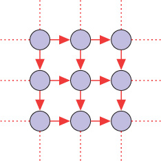
A graph G with nodes placed on the vertices of a 3 cross 3 grid is displayed. Every node in the grid points to the node to its right or bottom, if present. Dotted lines are extended from the corner nodes.

Figure 10.19. Graph G $?$ for Problem 21

22. Considering the gradient definition as in Problem 21, the p-Dirichlet form can be defined as

Sp(f)=1p∑i=1N||∇i(f)||p2. $\begin{matrix} S_{p} (?) = \frac{1}{p} \sum_{i = 1}^{N} | | \nabla_{i} (?) | |_{2}^{p} . \end{matrix}$

Prove or disprove

S2(f)=12(fTLinf+fTLoutf), $S_{2} (?) = \frac{1}{2} (?^{T} ?_{i n} ? + ?^{T} ?_{o u t} ?),$

where L_in is the in-degree Laplacian matrix and L_out is the out-degree Laplacian matrix of the graph.

23. Repeat Problem 11 for the directed Laplacian based DSP_G framework.

(a) Consider the filter in the frequency domain h(λ_ℓ) = a + mλ_ℓ, where λ_ℓ is an eigenvalue of the (in-degree) directed Laplacian of a graph. Can you represent the filter matrix in terms of the directed Laplacian matrix? If yes, find the filter matrix H for the case of (i) a = 0.5 and m = 1, and (ii) a = 2 and m = −1. Also plot the frequency responses of the filters for the graph shown in Figure 10.13.

(b) Consider a graph filter H = 0.4I + L + 3L². Determine if the filter H is LSI? Plot the frequency response of the filter for the graph shown in Figure 10.13.

1. For a directed graph, element w_ij of the weight matrix represents the edge weight directed from node j to node i (see Section 2.3.1 for details).

2. See Appendix A for deatils on norms.

3. When W is not diagonalizable, its Jordan decomposition can be used.

4. The classical convolution theorem states that convolution in the time domain is equivalent to multiplication in the frequency domain.

..................Content has been hidden....................

You can't read the all page of ebook, please click here login for view all page.

Table of Contents for 10 Graph Signal Processing Approaches

Create new playlist

Sign In

Sign Up

Chapter 10Graph Signal Processing Approaches

10.1 Introduction

10.2 Graph Signal Processing Based on Laplacian Matrix

10.3 DSPG Framework

10.3.1 Linear Graph Filters and Shift Invariance

Eigenfunctions of LSI Filters

10.4 DSPG Framework Based on Weight Matrix

10.4.1 Shift Operator

10.4.2 Linear Shift Invariant Graph Filters

10.4.3 Total Variation

10.4.4 Graph Fourier Transform

Frequency Ordering

10.4.5 Frequency Response of LSI Graph Filters

10.5 DSPG Framework Based on Directed Laplacian

10.5.1 Directed Laplacian

10.5.2 Shift Operator

10.5.3 Linear Shift Invariant Graph Filters

10.5.4 Total Variation

10.5.5 Graph Fourier Transform Based on Directed Laplacian

Diagonalizable Laplacian Matrix

Undirected Graphs

Frequency Ordering

Concept of Zero Frequency

10.5.6 Frequency Response of LSI Graph Filters

10.6 Comparison of Graph Signal Processing Approaches

10.7 Open Research Issues

10.8 Summary

Exercises

Table of Contents for
10 Graph Signal Processing Approaches

Chapter 10
Graph Signal Processing Approaches

10.3 DSP_G Framework

10.4 DSP_G Framework Based on Weight Matrix

10.5 DSP_G Framework Based on Directed Laplacian