Chapter 8
Spectra of Complex Networks
The eigenvalues and eigenvectors of a structure matrix of a complex network reveal information about its topology and its collective behavior. These structure matrices can be the adjacency matrix, weight matrix, Laplacian matrix, or random walk matrix of the graph representing a complex network. Studying the spectra, that is, the eigendecomposition of these matrices, leads to interesting results about the underlying network. For example, eigendecomposition of the Laplacian matrix helps in identifying communities (clusters) in a social network. Moreover, spectral densities of various complex network models follow specific patterns and, therefore, allow classification of networks. Furthermore, the eigenvalues of a structure matrix of a network provide frequency interpretation that is useful for analyzing data defined on the network. This chapter deals with the eigenvalues and eigenvectors of various matrices related to a graph, or indirectly to a complex network.
8.1 Introduction
The spectrum of a graph is the set of eigenvalues of a structure matrix representing the graph. These matrices include, but are not limited to, the adjacency matrix, Laplacian matrix, normalized Laplacian matrix, and random walk matrix. The spectrum of a graph is highly dependent on the form of the matrix and, therefore, depending on the structure matrix chosen, we can have different spectra for a graph. The graph spectrum has been widely used in graph theory to characterize the properties of a graph and extract structural information of the graph. An interesting property of the graph spectrum is that it is invariant to graph labeling; that is, no matter how vertices of the graph are indexed, the graph spectrum is unique. Therefore, the spectrum of the graph can be used as an alternative representation of a graph.
Most of the real-world networks are very large, containing thousands of nodes. For such a network, it is suitable to study their spectral density1 instead of the list of eigenvalues. It is observed that spectral densities (adjacency matrix as well as Laplacian matrix) of complex networks follow specific patterns. For example, spectral density of an Erdös-Rényi (ER) random graph follows semicircle law [138], [139]. However, for scale-free networks, the spectral density has a shape of a triangle with a power-law tail [140], [141]. Moreover, for small-world networks, the distribution of spectra consists of several sharp peaks [140]. Studying the spectral distribution of various complex network models not only provides a means for network classification, but also reveals various topological features of networks. For example, by estimating moments of the spectral density, one can calculate the number of various subgraphs [142].
There are various ways to represent spectral distribution of a matrix. Among those, a simple way to show the distribution of eigenvalues is to use a histogram plot or relative frequency plot with desired number of bins between the interval of [λmin, λmax], where λmin is the smallest magnitude eigenvalue of a structure matrix and λmax is the eigenvalue with largest magnitude. The second method to represent the spectral distribution is to convolve the impulse train (Dirac delta sum) with a smooth kernel g(λ, λi) and plot the density function
The smooth kernels can be Gaussian distribution or Cauchy-Lorentz distribution. When using a Gaussian kernel with a fixed variance σ2, the spectral distribution is represented by
Small values of the variance σ2 emphasize the finer details, whereas large values bring out the global pattern more conspicuously.
In the chapter, we discuss spectra of adjacency and Laplacian matrices of different graphs. Various bounds on the eigenvalues of the adjacency and Laplacian matrices are also discussed. Spectra of complex network models including random, small-world, and scale-free networks are discussed. Moreover, the connection between discrete Fourier transform (DFT) and eigendecompositions of adjacency and Laplacian matrices of a ring graph is highlighted.
8.2 Spectrum of a Graph
An N-node graph can be described using various structure matrices such as the adjacency matrix, Laplacian matrix, and random walk matrix. The set of (N number of) eigenvalues of a structure matrix of the graph is known as the graph spectrum. The spectrum of a graph does not depend on the labeling or indexing of vertices. Depending on the indexing of the vertices of a graph, the adjacency matrix may not be unique; however, the spectrum remains unaltered.
Example
Figure 8.1 shows different vertex indexings of a three-node path graph and their corresponding adjacency and Laplacian matrices. For all three cases, the adjacency matrix spectrum is and the Laplacian matrix spectrum is {0, 1, 3}.
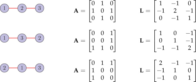
Figure 8.1. Different vertex indexings of a three-node path graph and corresponding adjacency and Laplacian matrices. For all the three cases, the graph spectrum (adjacency as well as Laplacian) remains unchanged.
Although the spectrum of a graph can reveal many characteristics of the graph, the structure of the graph cannot be uniquely determined from the graph spectrum. We may have two or more different graphs with the same spectra. The graphs having same spectra are called cospectral or isospectral graphs. For example, the graphs and shown in Figure 8.2 are cospectral graphs with respect to the adjacency matrix, since the eigenvalues of the adjacency matrices of both the graphs are {−2, 0, 0, 0, 2}. Note that, however, the eigenvectors of the adjacency matrices of the two graphs are different. For generating pairs of cospectral graphs, Seidel switching is a popular technique. Characterization by graph spectra is discussed in detail in [143], [144].
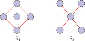
Figure 8.2. Cospectral graphs with respect to the adjacency matrix
Sometimes it is also beneficial to study the eigenvectors of a structure matrix of a graph. In Chapter 9, we will see that the eigenvectors of the Laplacian matrix of a graph act as graph harmonics that allow frequency analysis of signals defined on the graph. Moreover, eigenvectors of the graph Laplacian are also used in clustering of the graph (Section 8.5.5). For a three-node path graph, Figure 8.3 shows all the eigenvectors of the adjacency matrix and Figure 8.4 shows the eigenvectors of the Laplacian matrix. Note that all the eigenvectors have been normalized to have unit ℓ2-norms.
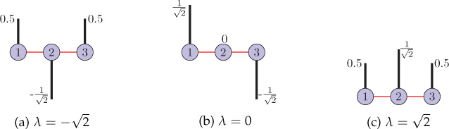
Figure 8.3. Eigenvectors of the adjacency matrix of a three-node path graph
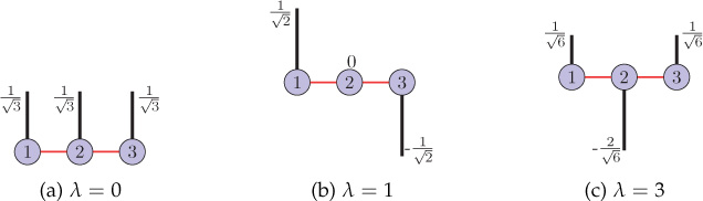
Figure 8.4. Eigenvectors of the Laplacian matrix of a three-node path graph
8.3 Adjacency Matrix Spectrum of a Graph
Adjacency matrix spectrum of a graph is the set of eigenvalues of the adjacency matrix of the graph. For an undirected graph, the adjacency matrix A is symmetric, and as a result, it constitutes N real eigenvalues. Let μ0 ≤ μ1 ≤ ... ≤ μN−1 be the eigenvalues of A. The sum of the absolute values of the eigenvalues of A is known as the graph energy. Some basic properties of the eigenvalues and eigenvectors of adjacency matrix for an undirected graph are as follows:
All the eigenvalues of the adjacency matrix are real.
The sum of the eigenvalues is zero, that is, .
The sum of the square of the eigenvalue is equal to twice the number of edges present in the graph, that is, .
The geometric multiplicity and algebraic multiplicity are same for every eigenvalue.
As the adjacency matrix is nonnegative, it follows from Perron-Frobenius theorem that the eigenvalue with maximum absolute value (which is always positive) has a multiplicity of one, that is, it has a 1 × 1 size Jordan block. Moreover, the corresponding eigenvector will be non-negative. If the graph is connected, the largest eigenvalue has a multiplicity of one.
The eigenvectors form a complete set of orthogonal basis.
8.3.1 Bounds on the Eigenvalues
The largest eigenvalue μN−1 of the adjacency matrix A of a graph is bounded by
where is the average degree, and dmax is the maximum degree of the graph.
Bounds Involving Chromatic Number
If is the chromatic number of a graph , then
and
where μ0 and μN−1 are the smallest and the largest eigenvalues of the adjacency matrix A of the graph , respectively.
8.3.2 Adjacency Matrix Spectra of Special Graphs
In this section, the adjacency matrix spectra of special graphs such as path graph, ring graph, star graph, complete graph, and bipartite graph are presented. Due to their special topological features, studying spectral properties of them can help one to identify and associate various spectal features and the associated topological characteristics. Definition of these graph types can be found in Chapter 2.
Path Graph
For a path graph with N vertices, the adjacency matrix has N distinct eigenvalues: , where k = 1, 2, . . . , N.
Cyclic (Ring) Graph
For a cyclic graph with N vertices, the adjacency matrix has N distinct eigenvalues: the complex n-th roots of unity, that is, , where k = 0, 1, . . . , N − 1.
Star Graph
For a star graph with N vertices, the adjacency matrix has three distinct eigenvalues: , 0 (with multiplicity N − 2), .
Complete Graph
For a complete graph with N nodes, the adjacency matrix has two distinct eigenvalues: −1 (with multiplicity N − 1) and N − 1.
Bipartite Graph
For a bipartite graph , the spectrum of the adjacency matrix is symmetric about zero; that is, for each eigenvalue μi, the value −μi is also an eigenvalue of the graph . An example bipartite graph is shown in Figure 8.5(a) and the corresponding adjacency matrix spectra is shown in Figure 8.5(b). Notice that the spectra is symmetric about zero eigenvalue.
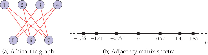
Figure 8.5. A bipartite graph and its adjacency matrix spectra
Directed Ring Graph
For a directed cyclic graph with N vertices, the adjacency matrix has N distinct eigenvalues: , where k = 0, 1, . . . , N − 1.
A directed ring graph has special importance for us, because it is the graph corresponding to a discrete-time periodic signal. The eigendecomposition of the adjacency matrix of a directed ring graph provides the idea of graph Fourier transform (GFT), discussed in the next chapters. The eigenvectors of the adjacency matrix of a directed ring graph are same as the columns of the classical DFT matrix. The N × N DFT matrix is
The adjacency matrix of an N-node directed ring graph can be diagonalized as
Figure 8.6 shows a directed ring graph and its adjacency matrix. The eigenvalues of the adjacency matrix are 1, 0.31 − 0.95j, −0.81 − 0.59j, −0.81 + 0.59j, and 0.31 − 0.95j. For the five-node directed ring graph, observe that
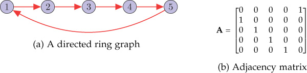
Figure 8.6. A directed ring graph and its adjacency matrix
where
Note that the diagonal entries in the diagonal matrix in Equation (8.3.6) are nothing but the eigenvalues of the adjacency matrix of the five-node ring graph. The eigenvalues of the adjacency matrix of a directed ring graph are the discrete frequencies corresponding to the DFT. Moreover, we will see in Chapter 10 that the eigenvectors of the weight matrix (adjacency matrix for unweighted graph) can be used to define the GFT.
8.4 Adjacency Matrix Spectra of Complex Networks
As discussed in Section 8.1, for large networks having more than a few thousand nodes, the numerical calculation of the spectra (eigenvalues) consumes significant time and memory. For such networks, spectral characterization is made using spectral density (distribution) function. The most straightforward way to obtain this density is to compute all eigenvalues of the matrix; however, this approach is generally costly and wasteful for large networks. There exist alternative approaches [145] that allow us to estimate the spectral density function at much lower cost. Discussion of these methods is out of scope of this book.
The spectral density of adjacency matrix of a network reveals its topological features. The adjacency matrix for an undirected network is symmetric and, therefore, its all the eigenvalues are real. One can also view the spectral density as a probability density distribution that measures the likelihood of finding eigenvalues near some point on the real line.
The ER model of random networks generates an uncorrelated graph because the presence or absence of an edge between two vertices is independent of the presence or absence of any other edge, so that each edge may be considered to be present with independent probability. For such uncorrelated random networks, from Wigner’s law [146], [147], [148], the spectral density can be approximated by a semicircular function. However, most of the real-world networks are correlated and are modeled as small-world or scale-free networks (Chapters 4 and 5). Small-world networks have a complex spectral density consisting of several sharp peaks, and scale-free networks constitute a triangle-like spectral density with a power-law tail [140], [139], [141]. Therefore, considering the pattern of the spectral density function, one can classify a network. Moreover, various structural properties can also be extracted from the spectral density function of a network. Now, we will discuss spectral density of each network type in detail.
8.4.1 Random Networks
As discussed in Appendix A.7, for an N × N uncorrelated random symmetric matrix M with (i) mean of each entry (which is a random variable) is zero (E[mij] = 0), (ii) variance of the non-diagonal entries is σ2 () and has finite higher order moments, then if N → ∞, the spectral density of M follows a semicircular distribution given as
The above result is known as Wigner’s law.
Wigner’s law is used to characterize the spectral density of ER random networks. For an ER random network with no self-loops, each non-diagonal entry of its adjacency matrix aij, for i ≠ j, is a bi-valued discrete random variable (0 with a probability (1 − p) and 1 with a probability p). Therefore, mean of the entry aij is given by
and the variance is
Observe that mean of an off-diagonal entry of the adjacency matrix is non-zero and, therefore, the condition of Wigner’s law is violated. However, for a positive mean, the spectral density follows semicircular distribution when properly rescaled [138], [140]. Only the largest eigenvalue μN−1 is isolated from the bulk of the eigenvalues and has a normal distribution with mean (N − 1)m + σ2/m = (N − 1)p + p (p − 1)/p = Np and variance 2σ2 = 2p(p − 1) [138].
Figure 8.7 shows the spectral density of a 1000-node random network generated using the ER model with edge probability of 0.1. The spectral distribution shown in the figure is averaged over 100 experiments. The plot is a histogram plot with 100 bins. In the plot, apart from the semicircular bulk, one can also observe a small peak which is separated from the bulk of eigenvalues.

Figure 8.7. Spectral distribution of a 1000-node ER network (p = 0.1) averaged over 100 experiments. The number of bins is 100.
8.4.2 Random Regular Networks
Here we discuss the distribution of eigenvalues of an N-node random d-regular graph, chosen uniformly at random from all d-regular graphs with N nodes. If d is fixed and N approaches infinity, then spectral density has a form
The above distribution is known as McKay law [149]. Figure 8.8 shows empirical spectral distributions of random d-regular graphs for various values of d.
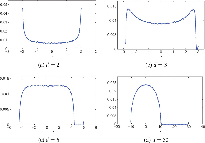
Figure 8.8. Spectral distribution of random d-regular networks with various values of d. Network size is 1000 nodes, and the distribution is averaged over 100 experiments. The number of bins is 100.
Further, it was proved that for d → ∞ and d ≤ N/2, the spectral distribution of a random d-regular graph follows semicircle law [150]. However, it is important to note that the semicircular distribution is achieved for even sufficiently large values of d. Figure 8.8(d) shows spectral distribution for d = 30. The semicircular spectral distribution is evident from the figure.
8.4.3 Small-World Networks
The adjacency matrix spectra of small-world networks contain multiple sharp peaks. In the Watts-Strogatz (WS) model or rewiring model of small-world networks, existing normal links (NLs) of a k-regular network are rewired to other nodes in the network based on a certain probability pr, where 0 ≤ pr ≤ 1 [6]. Details of the rewiring model can be found in Section 4.5.1. As the number of rewired links increases, small-worldness of the network also increases and the network tends to become random. With the increase in the rewiring probability, the sharp peaks in the spectral distribution become blurred and the spectral distribution tends to semicircular distribution.
For zero rewiring probability pr = 0, the small-world graph is regular and also periodical as each vertex is connected to its k-nearest neighboring vertices. Because of this highly ordered structure the spectra contains numerous singularities. The spectral distribution of such a network is plotted in Figure 8.9(a). In the figure, the network considered is 20-regular and has a total of 1000 nodes. One can observe several sharp peaks in the spectral distribution for pr = 0.
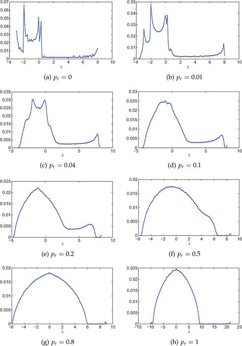
Figure 8.9. Spectral distribution of small-world networks with various rewiring probabilities pr. Small-world graph is generated using the Watts-Strogatz model starting with a 20-regular graph. Network size is 1000 nodes and the distribution is averaged over 100 experiments. The number of bins is 100.
When the rewiring probability is increased, the regularity of the network decreases and, therefore, the singularities are blurred and the spectal distribution tends to become smoother. The blurring of singularities with increase in rewiring probability can be observed from Figure 8.9(b–h). When the rewiring probability pr = 1, the network follows semicircular distribution, as shown in Figure 8.9(h). This is because for pr = 1, each link of the regular network is rewired and the network becomes completely random.
8.4.4 Scale-Free Networks
The adjacency matrix spectra of scale-free networks does not follow semicircle law. Consider the Barabási-Albert (BA) model of scale-free networks. According to the BA model of network generation, at time t = 0, there are m0 nodes present in the network. At each time instant, t, a new node is introduced to the network and m links are then connected to the existing network. The details of the BA model can be found in Section 5.5. Spectral distributions for scale-free networks, generated using the BA model, is shown in Figure 8.10. For each case, the network size is 1000 and the distribution is averaged over 100 experiments. In general, bulk of the spectral distribution has triangular shape for each case. Moreover, it constitutes power-law tails. For small values of m0, there is a sharp peak at zero eigenvalue. As the value of m0 increases, the sharpness of the peak decreases. It is important to note that both sides of the spectrum show long tails due to the slow decay of power law.

Figure 8.10. Spectral distribution of scale-free networks generated using the BA model. Network size is 1000 nodes and the distribution is averaged over 100 experiments. The number of bins is 100.
8.5 Laplacian Spectrum of a Graph
Spectrum of the Laplacian matrix of a graph is used in several applications of complex network analysis. A large number of the topological properties of a graph can be inferred from the spectrum of its graph Laplacian. For example, the eigenvalues and eigenvectors of the graph Laplacian allow frequency analysis of complex network data (detailed discussion on this topic is provided in the subsequent chapters). The Laplacian spectrum has also been used for measuring difference (or similarity) between networks. Moreover, the spectrum of the Laplacian can be used to detect community structures in a complex network [48]. Therefore, it is valuable to study the properties of the eigenvalues and eigenvectors of the graph Laplacian. The eigenvalues of the Laplacian matrix L are represented as λ0, λ1,... , λN−1 and the correspnding eigenvectors as u0, u1,... , uN−1, respectively. It is assumed that λ0 ≤ λ1 ≤ ... ≤ λN−1.
Some basic properties of the eigenvalues and eigenvectors of the adjacency matrix for an undirected graph are as follows.
All the eigenvalues of the Laplacian matrix are real and nonnegative.
It always has a zero eigenvalue.
If a graph is not connected, then the spectrum consists of the union of the eigenvalues of the connected components.
8.5.1 Bounds on the Eigenvalues of the Laplacian
We present a few important upper and lower bounds on the largest and smallest eigenvalues of the graph Laplacian. These bounds are very useful in characterizing the structure of a graph.
The second-smallest eigenvalue λ1 of the graph Laplacian L is upper-bounded by
In the above bound, the equality holds if the graph is complete. Moreover, from Gershgorin’s theorem (see Appendix A.8), the upper bound on the largest eigenvalue can be found to be
where dmax is the maximum degree of the graph. The above upper bound on the largest eigenvalue was improved in [151] as
where di represents degree of node i.
Bounds Involving Vertex and Edge Connectivity
For a non-complete N-node graph , λ1 is upper-bounded by
where and are vertex and edge connectivities of the graph, respectively [152].
Moreover, λ1 is lower-bounded by
Note that for an N-node path graph. Because for a connected graph, we can interpret from the above inequality that among connected graphs, λ1 is minimum for a path graph. As connectivity of a graph increases, λ1 also increases. Therefore, λ1 contains information regarding connectivity of a graph. More about this topic is discussed later in this chapter.
Bounds Involving Max-Cut Problem
For a graph with N nodes, maximum cut of , mc(), is bounded by
where λN−1 is the largest eigenvalue of the graph Laplacian [153]. Calculating max-cut of a graph is NP-hard and, therefore, the above bound is very helpful.
8.5.2 Bounds on the Eigenvalues of the Normalized Laplacian
The second smallest eigenvalue λ1 and the largest eigenvalue λN−1 of the normalized Laplacian Lnorm of a connected graph with N vertices are bounded by the following inequalities:
and
If a graph is not complete, then λ1 ≤ 1. Moreover, for every graph, λN−1 ≤ 2. For bipartite graphs, λN−1 = 2.
Bounds Involving Diameter
The diameter of a graph is upper-bounded by
where ⌈.⌉ represents the ceiling function. The diameter of a graph is an important structural parameter: for example, it is useful in estimation of maximum delay in a communication network. Knowing the Laplacian spectrum of the network, one can find out the upper bound on the graph diameter.
Bound Involving Cheeger Constant: Cheeger Inequality
For a connected graph , the second smallest eigenvalue λ1 of the normalized graph Laplacian is bounded by the following:
where is the Cheeger constant (refer to Section 2.7.1) of the graph. Moreover, an improved lower bound is given as .
8.5.3 Matrix Tree Theorem
A spanning tree of a graph is a subgraph that is a tree consisting of all the vertices of the graph. Using the spectrum of the Laplacian of a connected graph, the number of spanning trees can be calculated. This is given by matrix-tree theorem, which is stated as follows.
8.5.4 Laplacian Spectrum and Graph Connectivity
A graph is connected; that is, a path can always be found connecting one vertex to the other if and only if the smallest eigenvalue λ0 = 0 has multiplicity one. Moreover, the second smallest Laplacian eigenvalue λ1 of a graph is also important information contained in the spectrum of a graph. It is also known as spectral gap or algebraic connectivity [152] of the graph. The eigenvector corresponding to the algebraic connectivity is also known as the Fiedler vector. The value of λ1 is related to the connectedness of a graph: large values of λ1 are associated with graphs that are hard to disconnect. Moreover, the algebraic connectivity is non-decreasing; that is, adding more edges to the graph does not decrease the algebraic connectivity (see Exercise problem 4).
Community Detection Using Spectral Bisection
The eigenvalues and eigenvectors of the Laplacian can be used to detect communities in a network. The eigenvector corresponding to the second smallest eigenvalue, the Fiedler vector, bisects the graph into two communities based on the sign of the corresponding entry in the eigenvector. To divide a network into a large number of communities, one can use repeated bisection.
Consider a network that can be perfectly separated into k number of communities; that is, the edges exist only within communities and no edges exist between communities. For such networks, the Laplacian will be block-diagonal as follows:
Each diagonal block will form the Laplacian of its own component and, therefore, zero eigenvalue has a multiplicity of k. For example, consider a network shown in Figure 8.11. The network consists of two perfectly separating communities. The

Figure 8.11. A network with two communities
Laplacian of the network has zero eigenvalue with a multiplicity of 2, and the corresponding degenerate eigenvectors are
Observe the non-zero entries in the degenerate eigenvectors: the vertices corresponding to non-zero entries in each degenerate eigenvector form a community.
Now consider a case when the network does not separate perfectly into communities; that is, few edges exist between communities. In such networks, the Laplacian no longer remains block-diagonal and k − 1 eigenvalues are slightly greater than zero. Moreover, the second smallest eigenvalue λ1 can be used to measure the goodness of the split: smaller values correspond to better splits.
Let us consider a simpler case of bisection: there are only two communities in the network, but they are not well separated. Figure 8.12 shows two such networks. The second network (Figure 8.12(b)) has more intra-community edges than the first network (Figure 8.12(a)). Therefore, λ1 for the second network is more than that of the first network. The corresponding eigenvectors are

Figure 8.12. Addition of edges between communities in a network
respectively. Looking at the signs of the eigenvector entries for both of the networks, one can easily bisect the networks.
Although the spectral bisection method is fast, the main disadvantage is that it is limited to only bisection of a network. Division into a larger number of communities can be achieved by repeated bisection; however, this may not give satisfactory results. Moreover, in general, the number of communities is not known beforehand.
8.5.5 Spectral Graph Clustering
The eigenvectors of the graph Laplacian can also be utilized for clustering of graph nodes, and the method is polularly known as spectral graph clustering [154], [155]. Spectral clustering is one of the most popular modern clustering algorithms used by machine learning community. It has been extensively used for clustering of data points by creating a similarity graph from the data points and then utilizing the eigenvectors of the Laplacian matrix of the similarity graph. Spectral clustering outperforms traditional clustering algorithm such as k-means algorithm. In the field of complex networks, spectral graph clustering can be used for community detection.
Depending on which form of the graph Laplacian (unnormalized or normalized) is used, there exist multiple versions of the spectral clustering algorithms. Algorithm 8.1 describes spectral graph clustering that uses the unnormalized graph Laplacian L = D − W of a graph. Suppose we want to divide a graph into k number of clusters. For this purpose, first k eigenvectors of the graph Laplacian are computed to form the matrix Uk ∈ ℝN×k in which the eigenvectors are stacked as columns. Considering each row of Uk as a point in ℝk, these N points are divided into k number of clusters using k-means or any other clustering algorithm. Thus, the algorithm outputs k number of clusters.
Consider the graph shown shown in Figure 8.13 that has to be clustered into four clusters (the set of nodes inside a circle belongs to a cluster). The first four eigenvectors of the graph Laplacian are plotted in Figure 8.14. These eigenvectors can be stacked in a matrix Uk = [u0, u1, u2, u3] ∈ ℝ14×4. Each of the 14 rows in k, zi ∈ ℝ4, is treated as a point, and all 14 points are clustered into four clusters using k-means algorithm. The resulting clusters are the same as shown in Figure 8.13 using circles. A closer look at the plots of eigenvectors explains the working of the spectral graph clustering algorithm. Observe the signs (positive or negative) of the eigenvectors at each node. The signs of u1 (see Figure 8.14(b)) clearly divide the graph into two parts: nodes 1 through 4 and the rest. Next, the eigenvector u2, as shown in Figure 8.14(c), divides the rest of the nodes into two parts and identifies nodes 11 through 14 as one cluster based on their signs. Using u1 and u2, we could identify two clusters: nodes 1 through 4 and nodes 11 through 14. Finally, the signs of the eigenvector u3, as shown in Figure 8.14(d), at the remaining nodes (5 through 10) result in two more clusters: nodes 5 through 7 and nodes 8 through 10.

Figure 8.13. An example graph with four clusters
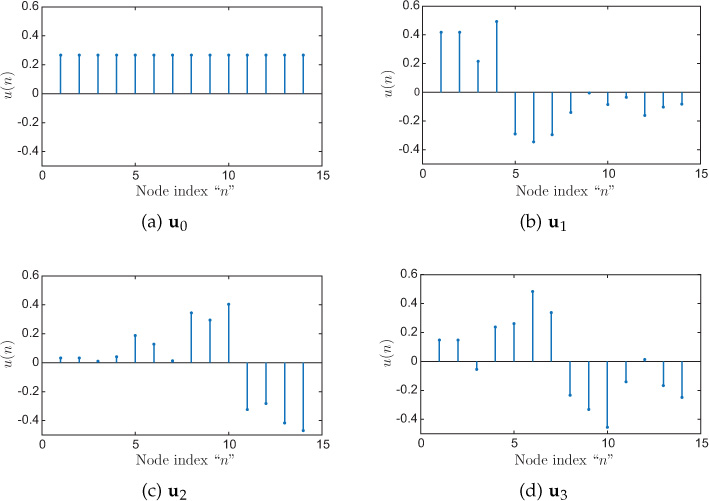
Figure 8.14. First four Laplacian eigenvectors of the graph shown in Figure 8.13
8.5.6 Laplacian Spectra of Special Graphs
The eigenvalues of a few special graphs such as path, ring, complete, and bipartite graphs are presented here.
Path Graph
For a path graph with N vertices, the graph Laplacian has N distinct eigenvalues: , where k = 0, 1, . . . , N − 1. Note that , which is the minimum among connected graphs.
The eigenvectors of the Laplacian are used in signal processing on graphs described in the next chapters. Figure 8.15 shows some of the eigenvectors of a 10-node path (string) graph. Notice that the variations in the eigenvector increase with the increase in the corresponding eigenvalues.
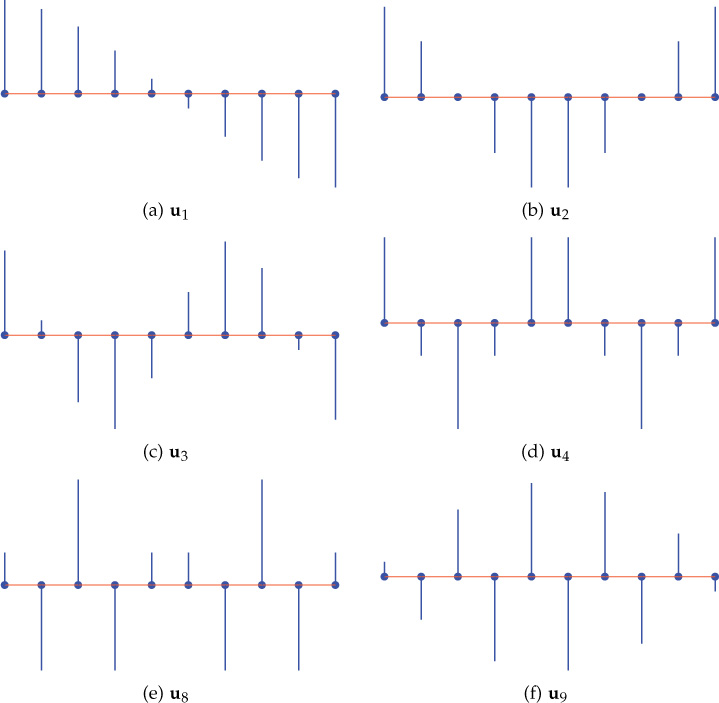
Figure 8.15. Laplacian eigenvectors of a 10-node path graph
The normalized graph Laplacian has N distinct eigenvalues: , where k = 0, 1, . . . , N − 1.
Cyclic Graph
For a cyclic graph with N vertices, the graph Laplacian has N distinct eigenvalues: , where k = 0, 1, . . . , N − 1. Moreover, one possible choice of the eigenvectors can be the columns of the DFT matrix given by Equation 8.3.4. For details of DFT, refer to Section 9.2.1.
The normalized graph Laplacian has N distinct eigenvalues: , where k = 0, 1, . . . , N − 1.
Star Graph
For a star graph with N vertices, the normalized graph Laplacian has three distinct eigenvalues: 0, 1 (with multiplicity N − 2), 2.
Complete Graph
For a complete graph with N nodes, the Laplacian matrix has two distinct eigenvalues: 0 and N (with multiplicity N − 1).
The normalized Laplacian matrix has two distinct eigenvalues: 0 and N/(N − 1) (with multiplicity N − 1).
Bipartite Graph
For a bipartite graph, the spectrum of the normalized Laplacian matrix is symmetric about 1; that is, for each eigenvalue λi, the value 2 − λi is also an eigenvalue. An example bipartite graph is shown in Figure 8.16(a), and the corresponding Laplacian spectrum is shown in Figure 8.16(b). Notice that the spectra is symmetric about unit eigenvalue.
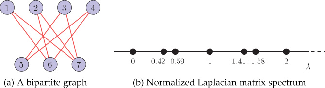
Figure 8.16. A bipartite graph and its normalized Laplacian matrix spectrum
8.6 Laplacian Spectra of Complex Networks
This section discusses spectral distribution of the Laplacian matrix of various complex network models including random networks, random regular networks, small-world networks, and scale-free networks. It will be observed that the shape of Laplacian spectra is the same as that of adjacency spectra for most of the cases. The only difference is the concentration of the bulk of the distribution toward large eigenvalues in the case of Laplacian spectra, as opposed to the smaller eigenvalues in the case of adjacency spectra. For scale-free networks, Laplacian and adjacency matrix spectra have different shapes.
8.6.1 Random Networks
Figure 8.17 shows the spectral density of a 1000-node random network generated using the ER model with edge probability of 0.2. The spectral distribution shown in the figure is averaged over 100 experiments. The bulk of the spectral distribution is located toward high eigenvalues and is close to semicircular distribution. Also, observe a small peak at zero eigenvalues, which is due to the fact that there is always a zero eigenvalue of the graph Laplacian.
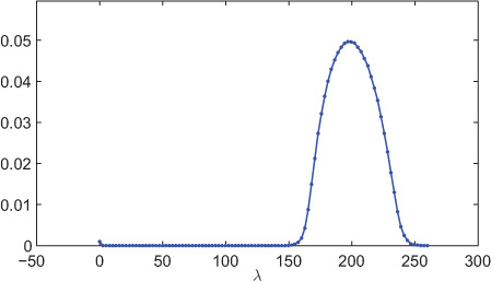
Figure 8.17. Spectral distribution (Laplacian) of a 1000-node ER network (p = 0.2) averaged over 100 experiments. The number of bins is 100.
8.6.2 Random Regular Networks
Recall from Section 8.4.2 that the adjacency matrix spectra of a random regular network was given by McKay law (Equation 8.4.4), and for large d, the distribution becomes semicircular. Notice that the bulk of the distribution is symmetric about zero eigenvalue. Figure 8.18 shows spectral distribution of random regular networks for various values of d. The Laplacian spectra also has the same shape as adjacency matrix spectra except that the bulk is concentrated toward large eigenvalues. Moreover, the Laplacian spectra becomes semicircular for large values of d with the bulk toward large eigenvalues, as can be seen from Figure 8.18(d).
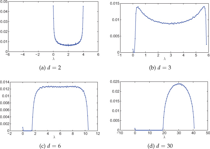
Figure 8.18. Spectral distribution (Laplacian) of random d-regular networks with various values of d. Network size is 1000 nodes and the distribution is averaged over 100 experiments. The number of bins is 100.
8.6.3 Small-World Networks
The Laplacian spectra of small-world networks follow same pattern as adjacency matrix spectra discussed in Section 8.4.3. The only difference is that the bulk of Laplacian spectra reside toward large eigenvalues, whereas bulk of adjacency matrix spectra reside toward small eigenvalues.
Figure 8.19(a–h) shows Laplacian spectra of small-world networks for various rewiring probabilities generated using the WS model. The small-world networks have been generated by rewiring a 1000-node 20-regular network. For small values of rewiring probabilities, the spectra contains a number of sharp peaks because of high regularity. As the rewiring probability increases, the network tends to random network and, therefore, spectra tends to follow semicircular distribution.
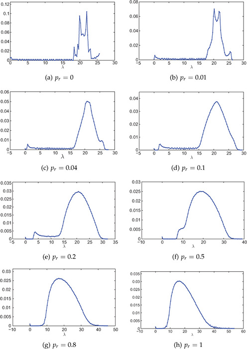
Figure 8.19. Spectral distribution (Laplacian) of small-world networks with various rewiring probabilities pr. The small-world network is generated using the Watts-Strogatz model starting with a 20-regular graph. Network size is 1000 nodes and the distribution is averaged over 100 experiments. The number of bins is 100.
8.6.4 Scale-Free Networks
Figure 8.20 shows Laplacian spectra of various scale-free networks generated using the BA model. For each case, the distribution has a peak near zero, implying that most of the eigenvalues are small.
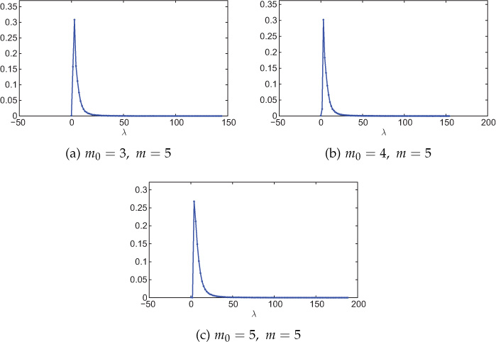
Figure 8.20. Spectral distribution (Laplacian) of scale-free networks generated using the BA model. Network size is 1000 nodes and the distribution is averaged over 100 experiments. The number of bins is 100. Here m0 is the number of nodes existing at the beginning of the network evolution, and m is the number of edges added in every time step between the newly added node and the existing nodes in the network.
8.7 Network Classification Using Spectral Densities
Adjacency and Laplacian spectra of various complex network models including random, small-world, and scale-free networks was discussed is Sections 8.4 and 8.6, respectively. Table 8.1 summarizes adjacency as well as Laplacian spectra for different complex network models. The shape of spectral distribution of a network can be used to classify the network.
Table 8.1. Spectral density of various network models
Network Type |
Adjacency Spectra |
Laplacian Spectra |
Random d-regular |
• Follows McKay law. Bulk of the distribution is symmetric about zero eigenvalue. • Semicircular distribution for large values of d, with bulk concentrated toward large eigenvalues. |
• Similar to adjacency matrix spectra, except bulk of the distribution is toward large eigenvalues. • Semicircular distribution for large values of d, with bulk concentrated toward large eigenvalues. |
ER |
• Follows semicircular distribution, with bulk around zero eigenvalue. |
• Follows semicircular distribution, with bulk toward large eigenvalues. |
Small-world |
• For small values of rewiring probability pr, the distribution consists of singularities. • As pr tends to 1, the distribution tends to become semicircular. |
• For small values of rewiring probability pr, the distribution consists of singularities. • As pr tends to 1, the distribution tends to become semicircular. |
Scale-free |
• Bulk of the distribution has triangle-like shape and has power-law tails. |
• Sharp peak at small eigenvalues. |
8.8 Open Research Issues
For a random network, the spectral density follows the semicircle law. However, such simple characterization of spectral density does not exist for small-world and scale-free networks. Although many structural characteristics of real-world network models such as WS small-world and BA scale-free models are well known, analytical results concerning their spectral properties remains an open question.
Very little is known about the effect of edge or vertex addition on the graph spectrum. Studying the change in the graph spectrum with change in the topology of a network is an open research area.
Although spectra of undirected networks has been studied well, very little is known about the spectra of directed graphs.
Using spectral density for modeling network evolution is an open research area. Some initial efforts in this direction can be found in [156], [157].
8.9 Summary
This chapter presented adjacency and Laplacian spectra of complex networks and special networks. The set of eigenvalues and eigenvectors provides useful information about the structure of a network. For example, connectivity, diameter bounds, isoperimetric constant, and community structure of a network can be deduced from the graph spectra. Moreover, the eigenvalues of the Laplacian and adjacency matrices provide frequency interpretation that is utilized in graph signal processing theory discussed in the subsequent chapters.
Spectral patterns of various complex network models including random, small-world, and scale-free were discussed. It was found that the spectral density can act as a means for network classification.
Exercises
1. Explain why the spectrum of a graph is independent of vertex labeling.
2. Prove the following:
(a) The Laplacian of an undirected graph has nonnegative eigenvalues.
(b) The eigenvalues of the normalized Laplacian of an undirected graph lie in the interval [0, 2].
3. Find the adjacency and Laplacian spectra of the graphs shown in Figure 8.21.
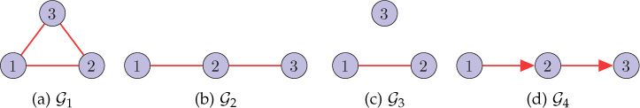
Figure 8.21. Example graphs (Problems 3 and 4)
4. Consider graphs and shown in Figure 8.21. From the adjacency and Laplacian spectra of the graphs, what can be commented on the connectivity of the graphs?
![]() 5. (a) Using eigendecomposition of the graph Laplacian, identify the three communities in the graph shown in Figure 8.22.
5. (a) Using eigendecomposition of the graph Laplacian, identify the three communities in the graph shown in Figure 8.22.
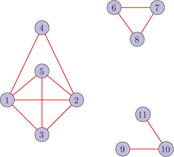
Figure 8.22. Graph (Problem 5)
(b) Repeat part (a) if there is an additional edge between nodes 4 and 6.
6. The Laplacian matrices of 10-node graphs are
List the adjacency and Laplacian matrix eigenvalues of the graphs. Also, plot the corresponding graphs.
7. Let be the Kronecker product of graphs and . Comment on the eigenvalues and eigenvectors of the adjacency and Laplacian matrices of .
What if is the strong product of graphs and ?
8. Let be the Cartesian product of graphs and .
(a) Determine the Laplacian eigenvalues of in terms of the Laplacian eigenvalues of and .
(b) Using the above result, find the Laplacian eigenvalues of the Cartesian product of a four-node star graph and a 3 node complete graph.
Hint: L = L1 ⊗ IN1 + IN2 ⊗ L2.
9. Prove that the total number of closed walks of length k in a graph is equal to , where μ0, μ1, ... , μN−1 are the eigenvalues of the graph adjacency matrix.
![]() 10. Generate a random sensor network having 1000 nodes. Compare the transition matrix spectra of the graph with adjacency matrix spectra.
10. Generate a random sensor network having 1000 nodes. Compare the transition matrix spectra of the graph with adjacency matrix spectra.
11. Prove that vector 1 (vector with all entries as 1) is an eigenvector of the adjacency matrix corresponding to eigenvalue k if and only if the graph is a k-regular graph.
12. Prove that a graph is regular (of degree μmax) if and only if . Here, μ0, μ1, ... , μN−1 are the eigenvalues of the graph adjacency matrix A and μmax is the largest eigenvalue.
Hint: Use Equation 8.3.1 for a regular graph.
13. Prove that
where di is the degree of node i and |ɛ| is the number of edges in a graph (μi and λi are eigenvalues of adjacency and Laplacian matrices, respectively).
14. Give a few examples of cospectral graphs with respect to the Laplacian matrix.
![]() 15. Generate three ER graphs: graph with 100 nodes and edge probability 0.08, graph with 150 nodes and edge probability 0.07, and graph with 200 nodes and edge probability 0.05. Ensure that each of the three graphs is connected. Now add 10 additional edges among these three graphs to create a single connected graph . Using the spectral clustering method, write a program to find three clusters in the graph . Comment on the clusters you identified and whether the clusters you found are same as , , and .
15. Generate three ER graphs: graph with 100 nodes and edge probability 0.08, graph with 150 nodes and edge probability 0.07, and graph with 200 nodes and edge probability 0.05. Ensure that each of the three graphs is connected. Now add 10 additional edges among these three graphs to create a single connected graph . Using the spectral clustering method, write a program to find three clusters in the graph . Comment on the clusters you identified and whether the clusters you found are same as , , and .
16. For an r-regular graph, establish the relationship between the eigenvalues of the adjacency and Laplacian matrices.
![]() 17. Plot spectral densities of the adjacency matrices for the following networks: (i) US Air-97 and (ii) CPAN [109]. Details on these networks can be found in Section 5.3. Comment on the types of the networks based on the shape of their spectral densities.
17. Plot spectral densities of the adjacency matrices for the following networks: (i) US Air-97 and (ii) CPAN [109]. Details on these networks can be found in Section 5.3. Comment on the types of the networks based on the shape of their spectral densities.
![]() 18. Plot spectral densities of the adjacency matrices for the following networks: (i) Diseasome [67] and (ii) Power Grid [6]. Details on these networks can be found in Section 4.4. Comment on the types of the networks based on the shapes of their spectral densities.
18. Plot spectral densities of the adjacency matrices for the following networks: (i) Diseasome [67] and (ii) Power Grid [6]. Details on these networks can be found in Section 4.4. Comment on the types of the networks based on the shapes of their spectral densities.
![]() 19. Repeat Problems 17 and 18 for the spectral densities of the Laplacian matrices.
19. Repeat Problems 17 and 18 for the spectral densities of the Laplacian matrices.
20. If we can label the nodes in a graph such that the Laplacian matrix of the graph is circulant, then such a graph is known as a shift invariant graph [158]. The eigenvectors of the Laplacian matrix of a shift invariant graph are the same as the columns of the DFT matrix. One example of a shift invariant graph is the ring graph. Draw two more shift invariant graphs and verify that the eigenvectors of the corresponding Laplacian matrices are the same as the columns of the DFT matrix. Also comment on the eigenvalues of the Laplacians of the shift invariant graphs.
![]() 21. (a) Starting with a 30 × 30 grid network, generate a small-world network using pure random addition of new links with probability 0.05. Plot the spectral densities of the adjacency as well as Laplacian matrices of the network. The spectral density plots should be averaged over 1000 experiments.
21. (a) Starting with a 30 × 30 grid network, generate a small-world network using pure random addition of new links with probability 0.05. Plot the spectral densities of the adjacency as well as Laplacian matrices of the network. The spectral density plots should be averaged over 1000 experiments.
(b) Starting with a 900-node 6-regular network, generate a small-world network using the WS model with the rewiring probability of 0.05. Plot the spectral densities of the adjacency as well as Laplacian matrices of the network. The spectral density plots should be averaged over 1000 experiments. Compare these plots with those in part (a).
1. A detailed discussion of spectral density of a matrix is provided in Appendix A.6.