Chapter 7
Small-World Wireless Sensor Networks

Chapter 6 discussed the formation and classification of small-world wireless mesh networks (SWWMNs). This chapter discusses another type of multi-hop relaying network, small-world wireless sensor networks (SWWSNs), where complex network concepts can be very useful. Wireless sensor networks (WSNs) form one of the areas in computer networks where application of small-world network characteristics can benefit the performance. End-to-end delay, throughput, network robustness, and application-specific design are some of the areas where SWWSNs benefit us. This chapter briefly introduces SWWSNs and presents their benefits. A number of existing approaches for designing SWWSNs are classified and presented before discussing a set of open research problems.

Figure 7.1. An example wireless sensor network

The WSN nodes consist of a small electronic device with a collection of sensors to sense a set of physical parameters of interest, a short-range radio transceiver to transmit and receive the sensed information, a data processing module for processing the sensed data, a network protocol stack for coordinating the communication among multiple sensor nodes, and an energy source. With the development of micro electro mechanical systems (MEMS), sensor nodes are becoming inexpensive and smaller in size to the extent that they can even be considered as disposable devices. Moreover, due to the low device cost, monitoring the entire operating region becomes feasible with dense deployment of the sensor nodes. In some application scenarios, where access to the operating terrain is difficult, the sensor nodes are dropped from air-borne platforms such as aircrafts or unmanned aerial vehicles (UAVs) for monitoring the parameters of interest. In such cases, the WSN nodes are designed with a network protocol stack that provides capabilities such as self-organization, self-reconfiguration, distributed routing, energy efficiency, and better robustness in communication.

The BS interfaces the WSN nodes with the rest of the world. That is, the BS receives the data sensed and forwarded by sensor nodes and then processes the data before forwarding them to the users for further applications. Therefore, BSs in most WSNs are almost static, or they are nodes with minimal or no mobility with much better computing, communication, and energy resources. Figure 7.1 shows a WSN with several nodes and only one BS; however, a real-world WSN may have one or more BSs.

Since WSN nodes typically have limited energy resources, designing energy-efficient WSNs is challenging. Moreover, nodes communicating with the BSs, using multi-hop relaying, consume more energy than those nodes that only sense and process the data. Another major issue is the fact that the average path length to BS (APLB) packets take to traverse from far away sensor nodes to the BS in a large WSN is quite large. Most WSN nodes have radio transceivers with very limited range; therefore, the communication packets from a distant WSN node need to traverse a large number of hops before the data can reach the BS. Therefore, APLB from WSN nodes to the BS needs to be reduced for better network performance.

By transforming a WSN to an SWWSN, the APLB value can be reduced, thereby, the network performance can also be improved. One of the popular techniques by which a WSN can be transformed to an SWWSN is to add a few long-ranged links (LLs).² Here, one point worth mentioning is that even when both WSN nodes and BSs are stationary, addition of LLs may not always be feasible.

One may argue that strategies for creating SWWSNs are almost identical to the strategies for creating SWWMNs discussed in Chapter 6. However, WSNs operate in very different operating environments, and the application scenarios are also different when SWWSNs are concerned. The key differences between SWWMNs and SWWSNs can be observed in the following scenarios: (i) mobility of nodes, (ii) traffic flow characteristics, (iii) node density, (iv) resource constraints, and (v) LL addition strategies.

In SWWMNs, wireless mesh routers are almost static or moving with minimal mobility, and they are responsible for path finding in the network, routing data packets to designated destinations, as well as monitoring and maintaining network connectivity. On the other hand, mesh clients such as mobile phones, laptops, PDAs, and similar user devices, are mobile in nature and are either originators or recipients of data packets. Therefore, SWWMNs can be considered as partial mobility networks. By contrast, SWWSNs deploy fixed sensor nodes that communicate over multi-hop wireless network to a fixed BS. Therefore, the network can be considered as a static network with very limited or no mobility.

The user traffic in SWWMNs flows between client devices as well as from client devices to the Internet gateways. Further, the traffic is typically generated for user communications such as Web-based data, voice, and video traffic. In many WMN deployment applications, mesh routers can be installed before the network is used. In such cases, it is easy to design and deploy SWWMNs by adding a small number of LLs among the stationary wireless mesh routers in the network. SWWMNs find application in broadband community networks, highway communication networks, civilian communication networks, disaster response networks, and tactical communication networks where size of the networks is mostly from low (10s) to moderate (100s) numbers of nodes.

In SWWSNs, the traffic flow is from the tiny sensor nodes to the BS or sink nodes. Traffic flow that gets terminated in WSN nodes is not intended. While the parameter of interest is APL that is estimated among all the node pairs in an SWWMN, in SWWSN APLB is the parameter of interest and is calculated using the shortest path length between the sensor nodes and the BS. Note here that in a WSN, the traffic flows from sensor nodes to the BS. Further, the amount of traffic generated by a WSN node usually comprises the sensed data, which is very small compared to the traffic originated by a WMN node (user data).

Further, in an SWWSN, thousands of tiny WSN nodes are deployed densely in the operating region where different types of sensing and monitoring tasks are performed in order to collect valuable data. Therefore, the density of nodes, defined as number of nodes per unit area, is typically high compared to an SWWMN. After collecting all data, WSN nodes process the raw data before transferring to the BS, which further processes and forwards the data to the data repositories on the Internet. Compared to SWWSNs, the density of nodes is low in SWWMNs. The high density of nodes requires efficient bandwidth and traffic management operations in an SWWSN. Therefore, density of nodes may also be considered as one of the parameters for SWWSN creation.

One most important differences between WMNs and WSNs is the very limited resources available to a WSN node compared to a WMN node. A WSN node has very limited processing power (10s of KHz to 10s of MHz), memory resources (a few KB to a few MB), transmission range (a few meters to 10s of meters), data transmission rate (10s Kbps to 100s of Kbps), and power source (3V battery, energy harvesting sources, or even energy scavenged from the surroundings). On the other hand, a WMN router has capability orders of magnitude better than WSN nodes. For example, a WMN router may have processors with 100s of MHz to 1 to 3 GHz, memory resources in the range of 10s of MB to 10s of GB, transmission range varies from 100s of meters to 10s of kilometers, data rates from 10s of Mbps to 100s of Mbps, and power source with capacity ranging from 12V, 6 ampere-hour battery to unlimited power supply from the mains.

Therefore, as the operating environment as well as type of data gathered by the WSN nodes are different, LL addition strategies in SWWSNs are also different in SWWMNs.

• Reduction in average path length to the base station (APLB) can be achieved by SWWSNs. Consider Figure 7.2 (a). The APLB of nodes S1 and S2 is 1, whereas that for nodes S4 and S5 are 3 and 4, respectively. The APLB of the network can be estimated as 2.2 hops. Now consider Figure 7.2 (b) where an LL is added between the BS and node S3. As a result, the path length from the nodes to the BS is reduced for all nodes except S1 and S2. Now, the APLB of the network can be found to be reduced to 1.6 hops. Thus the network has become smaller by about 0.6 hops!

  

  Figure 7.2. An example SWWSN transformation and APLB reduction

• Reduction in the end-to-end delay in data packet transmission can also be achieved in the SWWSNs. Consider the same example as shown in Figure 7.2. For a given APLB value of a network, obtained as number of hops, the average end-to-end delay can be estimated as

  (7.3.1) D=APLB×(Dq+DMAC),

  where D represents the average delay from nodes to the BS, D_q represents the average queuing delay per hop, and D_MAC is the average delay per hop due to medium access control as well as transmission at the link layer. For an SWWSN, the APLB reduction can contribute to lower D value given similar D_q and D_MAC. Therefore, a carefully designed SWWSN can achieve lower end-to-end delay performance in many practical systems.

• Reduction in energy consumption for a significant fraction of nodes can be achieved for transferring data packets from the WSN nodes to the BS.

  Consider the network topology shown in Figure 7.3(a) which consists of one BS and N WSN nodes. Assuming traffic flows exist from sensor nodes to the BS, resulting in a total of N traffic flows. The total number of transmissions, T_WSN, due to these N flows can be estimated as

  (7.3.2) TWSN=Σi=1Ni=N(N+1)2.

  

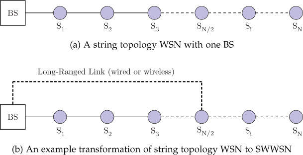
  Figure 7.3. Energy efficiency of SWWSN

  The total energy consumed by the nodes in a WSN, E_WSN, is proportional to the total number of transmissions made by the sensor nodes, and total energy consumed can be estimated as

  (7.3.3) EWSN=kTWSN=k×N(N+1)2,

  where k is a proportionality constant representing the energy consumption per transmission. Now, when the network is added with an LL between the node at location N/2 and the BS, the network energy consumption by the sensor nodes will be different. The LL can be made of a wired or wireless link. In the case of a wired link, it consumes much less transmission power than a wireless link. Assume that the LL consumes negligible energy for transmission. The nodes from S_N/2 to S_N communicate over the LL, resulting in the number of transmissions from those flows:

  (7.3.4) TN/2−N=Σi=0N/2(i+1),

  where the additional 1 is due to the transmission over the LL in order to reach the BS. Similarly, assuming the nodes from 1 to N/2 communicate over the regular links in the WSN to reach the BS, the number of transmissions is

  (7.3.5) T1−N/2=Σi=0N/2−1i.

  Therefore, the total number of transmissions in the network (i.e., T_SWWSN) due to the LL addition can be estimated as

  (7.3.6) TSWWSN=T1−N/2+TN/2−N=2(Σi=0N2−1i)+N2+N2+1.

  The energy consumed by the SWWSN can be estimated as

  (7.3.7) ESWWSN≈k×(2×Σi=0N2−1i+N2)+(N2+1)ELL.

  Upon simplifying the Equation (7.3.7), E_SWWSN becomes

  (7.3.8) ESWWSN≈k×N24+EnergyconsumedbytheLL.

  Note that the Equation (7.3.8) does not detail the energy consumed by the LL, and with the consideration of the energy required for the LL for transmission, E_LL, the total energy required can be found as

  (7.3.9) ESWWSN≈k×N24+(N2+1)ELL.

  Now, from Equations (7.3.3) and (7.3.9), the energy savings, E_S, due to the transformation of the WSN to an SWWSN, can be estimated as

  (7.3.10) ES=EWSN−ESWWSN.

  That is,

  (7.3.11) ES≈k×N(N+1)2−[k×N24+(N2+1)ELL].

  Simplifying Equation (7.3.11), it can be found that

  (7.3.12) ES≈kN(N+2)4−(N2+1)ELL.

  Therefore, the transformation of the WSN to an SWWSN can result in positive energy savings when ELL×(N2+1)<kN(N+2)4.. Careful design and implementation of the LL in this case can result in not only APLB reduction but also energy consumption savings.

• WSN to SWWSN transformation enhances the lifetime of most nodes in the network. Consider the SWWSN shown in Figure 7.3. From Equations (7.3.3) to (7.3.9), it can be found that the average energy consumed for transmissions in the network is lower (see the following example). Due to the lower energy consumption, average lifetime of nodes can be extended as well.

  ---

  Example

  Consider the network in Figure 7.3 where N = 10 and E_LL is negligible. The energy consumed in the unmodified network can be estimated as EWSN=k×N(N+1)2=k×55.. On the other hand, in the modified network to achieve SWWSN, the ESWWSN=kN(N+2)4=30k.. It can be found that the average energy consumed is reduced to 54%. That is, the average energy consumed is almost half. This lower energy consumption can result in increase in the lifetime of the nodes in the network.

  ---

• SWWSN enhances the end-to-end traffic flow performance such as throughput and latency between WSN nodes and BS in the network. Throughput achievable in a network is inversely proportional to the end-to-end latency or delay. As it can be observed that the APLB reduction results in lowering the average end-to-end delay, the SWWSN can achieve higher throughput and lower delay.

• Scalability of a very large WSN can be improved using the SWWSN approach. Scalability refers to the ability of a WSN to retain the network performance irrespective of a very large number of nodes. Due to the use of the SWWSN approach, a network can achieve lower resource consumption in terms of bandwidth, energy, and other resources. Due to the lower consumption of resources, the network scalability improves.

• Design and deployment of a WSN can be easier in sparse field deployments following an SWWSN approach. Sparse field deployments deal with much larger area with low density of nodes. Ensuring multi-hop wireless connectivity using short-range radios can be difficult in such sparse areas. However, for some nodes with the capability of operating the LLs, sparse WSNs is feasible with high efficiency.

• In many deployments, WSNs may not follow the node distributions characterized by the Poisson point process or neighbor degree distributions characterized by Erdös-Rényi (ER) random or scale-free networks. Therefore, neighbor degree relationship of nodes in a WSN depends on the transmission locality due to the limited radio transmission range. Therefore, the degree distribution of nodes, connectivity of nodes, and other network parameters need to be estimated considering the limited transmission range as well as the propagation characteristics of the operating environment.

• Most WSN nodes have only one radio interface, but in transforming WSNs to SWWSNs, some of the nodes, called high sensor (H-sensor) nodes, need to have at least two radio interfaces, one operating at the short transmission range and another operating at the longer transmission range. Making low-power devices with multiple interfaces is expensive, so the cost of network nodes can be high.

• WSNs are known for highly constrained nodes in terms of computing resources such as processor and memory resources. Making the network an SWWSN may demand higher resources for at least a subset of nodes. For example, the nodes with LLs may face higher traffic, demand larger buffers, and require more processing ability. Without considering the computer resource requirements, the LLs may result in performance bottlenecks.

• Nodes in a WSN have very limited transmission ranges and high energy constraints; therefore, transforming a WSN to an SWWSN requires at least some nodes to LLs that need to operate at much higher transmission ranges. Such LLs consume a higher amount of energy than normal links that use shorter transmission ranges.

  The transmission power, P_t, required to achieve a communication range R is proportional to R⁻β where β is the path loss exponent. Consider a situation where P_t is raised to Pt′ in order to achieve a k times higher transmission range, R^′, such that R^′ = kR. Therefore, given the same environmental factors and path loss exponent, it can be seen that

  (7.4.1) Pt′=Pt×(R′R)β=Pt×(kRR)βPt′=Pt×kβ.

  Note that depending on the value of k, the transmission power required can be very high. Such high power requirements result in either a limited number of design possibilities or new solutions where LLs can be created using highly directional antennas.

  ---

  Example

  For achieving an LL transmission range of four times longer than a normal WSN link, the transmission power required is about 16 times more than that of the normal link when β is 2. Since WSNs are highly energy constrained, creating LLs is a very challenging issue, and WSN nodes require special designs with additional power sources to form LLs.

  ---

  Note that the formation of LLs can also be carried out using wired links or optical point-to-point links, which require lower transmission energy than wireless LLs.

• Wired LLs are suitable in some SWWSN deployments where transmission energy is an issue. However, wired LLs also offer certain challenges. First, the use of wired LLs requires the nodes to have a wired network interface such as RJ45 or RJ11 ports. Adding an additional network interface can increase the cost as well as the physical size of the sensor nodes. Another issue with wired LLs is the need for long cables deployed in the terrain of network operation. For a network covering a large operating terrain, similar length cables are needed. In such cases, additional wired network relays may be needed to ensure the communication over the cables is satisfactory. Further, the physical deployment of cables in the operating terrain can be a very laborious task compared to wireless LLs. Once deployed, the network reconfiguration is also a very cumbersome task in wired LL-based SWWSNs.

• Due to the possibility of only a limited number of nodes that can have LLs, the simpler design approaches such as random node selection for LL creation cannot be carried out in a WSN. Therefore, complex design choices are needed for many deployment scenarios of SWWSNs.

• The SWWSN also must handle the complex issue of channel allocation due to the possibility of interference among the LLs that use wireless transmission. The channel allocation algorithms need to consider the physical layer characteristics of the LLs as well as normal links (NLs). For example, the channel allocation for omnidirectional LLs may not work efficiently for LLs based on directional antennas

• Application deployment–specific SWWSN design is essential. The LL creation needs to consider the traffic pattern that exists in a WSN, which is very different from other network forms such as social networks, WMNs, and the Internet. In WSNs, the traffic flow is either from the WSN nodes to the BS or from the BS to the sensor nodes. That is, the BS acts as the source node or sink node of all end-to-end communication flow. In some WSNs, where data fusion or information fusion is employed, the fused data may eventually be consumed by the BS. The LL addition process in SWWSN may need to consider the traffic flow in the network.

  Based on the application deployment, the topology of the network may also be influenced. For example, the string topology–based SWWSN may need a different design approach than an arbitrary topology–based SWWSN.

• Design of SWWSNs must be carefully carried out such that situations such as the Braess paradox [127] may not occur. The Braess paradox refers to a situation in networks where adding a new link may result in degradation of performance. For example, in a road network, creating a new road may result in reduction of APL; however, it may result in an increase in overall travel time due to the fact that many drivers choose to take a shorter path, resulting in high congestion and waiting time. In SWWSNs, it is particularly challenging due to the use of wireless channels. For example, when LLs and NLs share spectrum, their overlap can result in a higher number of collisions, leading to the wastage of bandwidth.

Wired links can be used for creating LLs in a variety of SWWSNs. Wired LLs can be accomplished by creating long-range cables such as Ethernet cable (e.g., RJ45) with repeaters or telephone cables (e.g., RJ11) with appropriate modems used to interface with the SWWSN nodes.

Another technology option for LL creation is to use omnidirectional wireless links. This type of LL can be achieved either by (i) increasing the transmission power of the wireless radio interfaces, thereby increasing the range, or (ii) using another wireless communication network, such as cellular networks, for LL creation. Existing omnidirectional radio transceivers can be enhanced with higher-gain power amplifiers to increase the range so that the requirements of an LL can be met. Alternatively, for a low-transmission range SWWSN, cellular network radios can be used for achieving LL communication between selected SWWSN nodes. The key benefit of the omnidirectional wireless LLs is the minimal complexity in forming the LL and, therefore, the design of SWWSN. The major disadvantage of using omnidirectional LLs is the high interference that may happen among the LLs as well as LLs and NLs.

In addition to the omnidirectional wireless network–based LLs, another way that is popularly considered for LL creation is to use point-to-point radio links using directional antennas. Compared to the omnidirectional wireless LLs, the directional LLs can face complexities in the design and deployment phase; however, the key advantage is the reduction in the interference caused by the LLs.

Finally, satellite-based communication links can also be utilized for the creation of LLs in an SWWSN. Packet-switched satellite links that use low data rate are available as commercial services for providing LLs. Many example technologies are commercially available in the market.

Iridium 9602 is one example of such a modem that can be used for SWWSN design and deployment [128]. Some of the technical specifications of this modem module are as follows: (i) very small form factor (size: 41mm×45mm×13mm) with a weight of only 30g, (ii) frequency band: 1616-1626.5MHz with time division duplex (TDD) method and TDMA/FDMA multiplexing method, and (iii) power consumption as follows: average idle current of 45mA, peak idle current of 195mA, peak transmit current of 1.5A, average transmit current of 190mA, peak receive current of 195mA, average receive current of 45mA, average current for message transfer of 190mA, and average power for short burst data (SBD) message transfer 1.0W. Such a modem can be interfaced with SWWSN nodes to achieve LL capabilities through an Iridium M2M satellite service. SBD messages of size 340 bytes generated by SWWSN nodes and messages of size 270 bytes received by SWWSN nodes can provide LL connectivity with a uniform global latency of less than 1 minute.³ Similar to the Iridium 9602 modem, the Iridium 9603 modem [129] as well as the currently planned device Iridium Edge [130] can also be used for LL creation in SWWSNs.

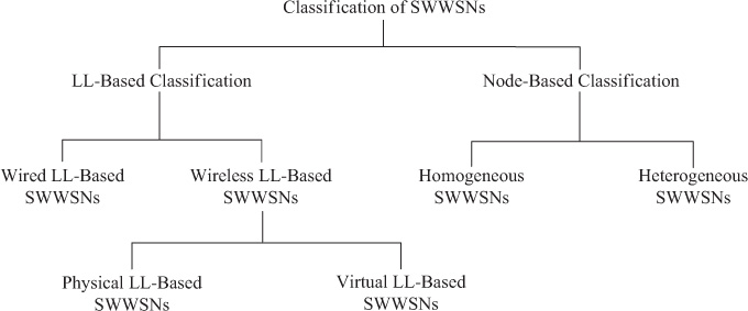
Figure 7.4. A classification of SWWSN formation approaches

Existing approaches for SWWSN formation based on the type of links can be further classified into two categories: wired and wireless LL-based approaches. In a large sensor field with stationary sensors, where the wired infrastructure is feasible for deployment, then a wired LL-based approach is a reliable method to create an SWWSN. In WSNs where wired LLs are infeasible or in the case of existence of sensor mobility, wireless LLs are the only realistic solution. Wireless LL-based approaches are classified into two further categories: heterogeneous and homogeneous SWWSNs. Heterogeneous SWWSNs have certain WSN nodes that are more capable than the rest of the WSN nodes in order to form the LLs, whereas each WSN node is expected to have LL realization capability when homogeneous SWWSNs are concerned. Another classification of the wireless LL-based nodes is on the basis of the physical or virtual nature of the LLs that are formed in an SWWSN. For example, in certain SWWSNs, a physical wireless LL may be formed, and in the rest, a virtual wireless LL may be formed. One example of forming virtual LL-based SWWSNs is to use UAVs to create temporary periodic or aperiodic LLs for creating backbones or LLs for gathering data. A detailed description of the existing approaches to transform a WSN to an SWWSN is presented later in this chapter.

where S is the set of all nodes in the network, N is the number of nodes, and d(i, BS) is the shortest path length from node i to its nearest BS.

APLB ratio is defined as the ratio of APLB of an SWWSN to its corresponding WSN without the LLs. For example, the APLB ratio can be termed as APLB reduction factor and is obtained as APLBSWWSNAPLBWSN and it indicates the fractional APLB reduction obtained due to the transformation to an SWWSN. Further, the quantity 1−APLBSWWSNAPLBWSN estimates the quantum of reduction in the APLB due to the transformation of a WSN to its SWWSN.

For conducting performance evaluation of an SWWSN with certain parameters such as number of LLs or length of LLs, an additional reference to the parameter can be used. For example, the APLB_SWWSN(k) refers to the estimated APLB value of an SWWSN after adding k LLs. The APLB ratio is represented as

where APLB(k) and APLB(0) represent the APLB of WSN networks with k and 0 LLs, respectively.

There are two possible reasons for LL saturation. First, the constraints placed for the addition of LLs may result in no further LL additions. For example, in the inhibition-distance-based SWWSN discussed in Section 7.6.10, every new LL is added to the network based on the positions of existing LLs and the nodes inhibited by the inhibition-distance parameter. Therefore, after adding a very small number of LLs, the strategy may permit no further LL addition. In such cases, the WSN is saturated with LLs due to the nature of the LL addition strategy. The N_Sat value may depend on the number of nodes in the network, the strategy used for LL addition, and the characteristics of the LL.

Second, the performance improvement due to the addition of new LLs may be negligible such that there exists no justification for further LL addition. In networks with a large number of nodes and where the LL addition strategy does not apply hard constraints, continuing addition of LLs may not benefit the network performance. In such cases, experiments can be conducted to identify the performance benefit of the LL addition and thereby identify the LL saturation point.

Figure 7.5. An example transformation of a string topology WSN to an SWWSN

Figure 7.5(b) shows the string topology WSN transformed to an SWWSN by using one LL between the node S_N/2 to the BS. Assuming the LL is a wired or wireless link, the APLB from the nodes to the BS can be estimated by considering the traffic for (i) the segment formed by the nodes from S_N/2 to S_N that use the LL to communicate to the BS, (ii) the segment formed by the nodes from S_N/4 to S_N/2 that use the LL to communicate to the BS, and (iii) the segment formed by the nodes from S₁ to S_N/4 that use the string topology WSN to communicate to the BS. The APLB can be estimated as the average of the APLB of each of these three network segments.

APLB of nodes in the network segment formed by the nodes S_N/2 to S_N can be estimated as follows:

Similarly, APLB of nodes in the network segment formed by the nodes S₁ to S_N/4 can be estimated as follows:

Finally, APLB of the network segment formed by the nodes S_N/4 to S_N/2 can be estimated as follows:

Therefore, APLB of the network can be estimated as the average of the APLBs for the three segments, mentioned earlier, and it can be approximated as N5.

That is, by adding one LL between node S_N/2 and the BS, the APLB can be reduced to approximately 3N16≈0.19N, which is lower than N5. Adding more LLs to the string topology WSN can result in further improvements in APLB. Therefore, transforming a string topology WSN to an SWWSN can improve the APLB, thereby also improving the throughput and delay performance.

Figure 7.6(a) shows a ring topology WSN with N nodes and a single BS. Nodes S₁ to S_N are organized in a ring topology so that every WSN node has two neighbors. The APLB of this topology can be estimated as follows. The furthest node from BS is S_N/2. Therefore, the network can be considered as two segments: (i) the segment consisting of nodes S₁ to S_N/2 and (ii) the segment consisting of nodes S_N/2+1 to S_N. Note that depending on whether N is even or odd, there can be a minor situation where each segment has the same number of nodes or one segment has one node more than the other segments. Neglecting such boundary issues, it can be assumed that each segment of the ring network has exactly the same number of nodes, resulting in the same APLB value for each segment. Therefore, in each of these segments, the furthest node is located at N/2 hops away from the BS, and the APLB value of each segment can be estimated as follows:

Figure 7.6. An example transformation of a ring topology WSN to SWWSN

That is, the APLB value of the ring topology WSN can be approximated as^N₄. Figure 7.6(b) shows the ring topology WSN included with an LL between the node S_N/2 and the BS. The addition of the LL transforms the network to an SWWSN. The addition of the LL contributes to the redundancy and robustness of the network besides making the network smaller in terms of APLB. For estimating the APLB of the network, we can find that the network has four segments: (i) nodes S₁ to S_N/4, (ii) nodes S_N/4 to S_N/2 which use the LL to communicate to the BS, (iii) nodes S_N/2 to S_3N/4 which also use the LL to communicate to BS, and (iv) nodes S_3N/4 to S_N. Each of these segments can be found to have an APLB of ≈N8 making the entire network APLB as ≈N8.

It is possible to add more LLs to further improve the APLB performance of an SWWSN. However, LLs should be added strategically so that the benefits can be substantial. Figure 7.7 shows the a ring topology SWWSN with two LLs. In Figures 7.7(a) and 7.7(b), LLs are added in two different ways. The addition of the two LLs as shown in Figure 7.7(a) does not provide any additional benefits compared to the case shown in Figure 7.6(b).

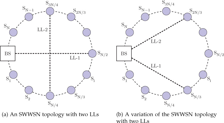
Figure 7.7. Examples of ring topology SWWSN with two LLs

The topology in Figure 7.7(a) provides an APLB of ≈ N/4 only. However, the second added LL (LL-2) does not provide any additional value. On the other hand, consider Figure 7.7(b) where the two LLs, LL-1 and LL-2, are added in a slightly different manner, from the BS to S_N/3 and S_3N/4, respectively. The configurations of two LLs result in substantial reduction in APLB, compared to Figure 7.7(a). In particular, the APLB of the network comes down to ≈N12 due to the addition of the two LLs, as shown in Figure 7.7(b).

Figure 7.8. An example grid topology SWWSN

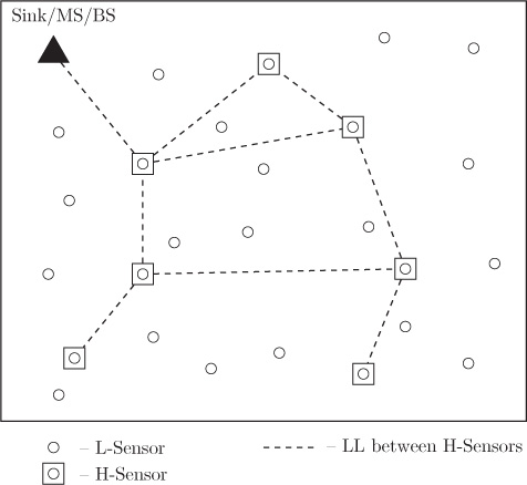
Figure 7.9. An example SWWSN created by RM-SWWSN approach

The key disadvantages of RM-SWWSN approach are that (i) the random selection of H-sensors for creating LLs does not take into account the specific traffic pattern present in the network, resulting in poor reduction in APLB, and (ii) the interference between the LLs may cause performance degradation, resulting in poor improvement in the overall performance.

where d(i, j) is the Euclidean distance between WSN nodes i and j, p_h is the highest LL addition probability to be considered in the SWWSN formation, and r is a structural parameter used for controlling the LL addition. For example, when r = 4 and p_h = 1, the denominator of Equation (7.6.8), capturing the Euclidean distance between two nodes in terms of hops, will have significant impact on p. When r = 2, we can obtain an LL addition probability similar to the Kleinberg model (see Section 4.5.3).

Once the link addition probability is determined, an LL addition has another hard constraint set by the transmission range limit of the H-sensors. That is, a chosen H-sensor pair for LL addition is discarded if

where Tx_range(i, j) and E(i, j) are, respectively, the transmission range of the H-sensors and the Euclidean distance between H-sensors i and j. Therefore, it can be seen that the actual probability of adding LLs in the network is lower than p value estimated in Equation (7.6.8). Experiments find that the number of H-sensors required to achieve effective small-world features when using NWSWWSN model is about 15%.

Note that LLs have both the lower and upper transmission limits. The lower transmission limit is set equal to a value higher than the transmission range of L-sensor nodes. The reason for this lower transmission limit is mainly that H-sensors are resource-expensive nodes and, therefore, using a transmission range equal to the L-sensor nodes may not help achieve small-world properties. The maximum range of an LL is also limited by the transmission range of the LL interface of an H-sensor. Despite the fact that the maximum and minimum transmission ranges determined for LLs are limited, energy efficiency can further be achieved by the application of power control.

In Kleinberg model–based SWWSNs, power control for an LL can be achieved over each of the LLs by exchanging messages with location information or by extracting the transmit power and received signal strength. Each H-sensor end point sends Hello messages to the other end point of an LL, with its location information included in the message. By exchanging the location information, transmission power is reduced sufficiently to maintain the connectivity of LLs. That is, the transmit power is limited to the amount required to maintain the connectivity of the LL. It is likely that not all H-sensor nodes have location information gathering capability. All H-sensor nodes that do not have location information gathering capability use the received signal strength indicator (RSSI) information to achieve power control.

From the simulation experiments it can be seen that an APL reduction of 45% can be achieved in a WSN field of 2000 nodes distributed in a 1000m × 1000m area where each node has an average neighbor degree of 15. In the experiment, the L-sensor nodes are taken with 60m transmission range, whereas the H-sensor nodes have maximum LL transmission range of 300m. When p_h = 1and r = 2, the number of H-sensors required to achieve effective small-world features is about 26%.

The main disadvantages of the Kleinberg SWWSN, in comparison to the NWSWWSN, include (i) higher APL and (ii) higher end-to-end latency. One of the reasons behind the higher end-to-end latency is that the key characteristics of LL formation in the Kleinberg model decrease the probability of LL addition when distance between nodes increases. Further, the Kleinberg model uses (iii) a larger number of H-sensor nodes and achieves lower value in latency with a given number of H-sensors.

The DRM, for creating an SWWSN, uses the following four steps to transform the network to an SWWSN:

• Step I—Creation of H-sensor neighbor tables (NTs).

• Step II—Selection of H-sensor neighbors to create a directed neighbor table (DNT).

• Step III—Formation of directed random LLs.

• Step IV—Interference-less channel allocation for the created LLs.

In the following, each of these steps are explained in detail:

• Step I—Creation of H-sensor NTs: In this step, an NT of H-sensors is created for each H-sensor i (as shown in Figure 7.10) in the network. Each H-sensor node sends Hello messages that contain its NodeId and geographic position over the H-sensor interface. When an H-sensor node receives such Hello messages, it creates an NT that contains the NodeId and position of its neighborhood H-sensors. Due to the fact that sensor nodes lack mobility, the Hello messages need not be transmitted in a periodic manner. However, the NTs are required to be re-created if events such as network reconfiguration or node failures happen.

  

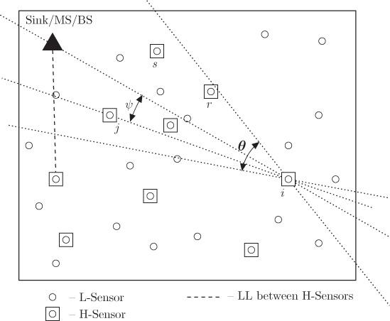
  Figure 7.10. Determination of directed LLs in DRM-SWWSN model

• Step II—Selection of H-sensor neighbors to create a DNT: In this step, a DNT is created for each H-sensor i (Figure 7.10) in the network. That is, a subset of the H-sensors in the NT of each node is selected due to their geographic position in the direction of the BS. Algorithm 7.1 is used for identifying the membership of the DNT.

• Step III—Formation of directed random LLs: In this step, random LL creation is carried out with the nodes in the DNT. Each H-sensor node with probability p chooses another H-sensor node in its DNT and sends a CREATE_LL packet for creating an LL with the node. In response to that packet, the requested node may send an ACK_CONFIRM packet or NACK_CONFIRM packet. The probability p is chosen based on the Klein-berg small-world model where p can be estimated as

  (7.6.10) p=1D(i,j)γ

  where D(i, j) is the distance between two candidate H-sensors i and j (see Figure 7.10), and γ is the scaling factor which is set as 2 in this case. The choice of p ensures that a longer range LL is created with lower probability compared to a medium range LL. Once a node is chosen, the ACK_CONFIRM packet is sent if the requested packet is available for creating an LL. On the other hand, the NACK_CONFIRM packet is sent in if the recipient of CREATE_LL already has LLs such that it cannot accept any more requests. In the case of ACK_CONFIRM response, both the nodes proceed with the formation of an LL between them. However, in NACK_CONFIRM, the H-sensor node that initiated CREATE_LL attempts forms an LL with another randomly selected node in its DNT.

  The random selection of DNT nodes for the formation of an LL continues until the H-sensor node forms an LL. It is possible with a low probability that an H-sensor node cannot easily find a DNT member to form an LL. The DRM-SWWSN approach additionally suggests forcing the formation of an LL with a DNT member by following a RECOVERY_LL process. In the RECOVERY_LL process, an H-sensor can send a FORCE_CREATE_LL message to its DNT member where the recipient is forced to create an LL by breaking its existing LL, if any.

  Algorithm 7.1 Algorithm for Creating Directed Neighbor Table for H-sensors in DRM-SWWSN

  Require:

  NT — Neighbor table of the given H-sensor

  1: Estimate the parameters of the line Y = aX + b formed by the H-sensor i and the BS

  2: Estimate the lines that form angle θ where the line Y = aX + b bisects the angle θ

  3: for Each H-sensor i ∈ NT do

  4: Estimate the parameters of the line, Y_i = a_i X + b_i, formed by node i and the BS

  5: Calculate the tangent of the angle formed by the line formed by H-sensor i by using ψi=ai−a1+aia

  6: end for

  7: DNT = ∀_i ∈ NT where tanψi<tanθ2 // All H-sensor neighbors within the angle tan θ2 is chosen to form DNT

• Step IV—Interference-less channel allocation for the created LLs: Channel assignment for the LLs is carried out in this step. The DRM-SWWSN approach utilizes an interference graph or conflict graph approach for assigning channels for the LLs. In this conflict graph approach, a graph ?′ is modeled as ?′=(?′,ℰ′), where the set of LLs is modeled as a set of nodes, ?′. The edges in ?′ are defined by the interference possibility between LLs. That is, if there is an interference between two LLs, then there is a corresponding edge in the edge set ℰ′ in the graph ?′. A channel is assigned to an LL in such a way that it does not interfere with other LLs using the same channel. Note that the channel allocation is carried out by the BS in a centralized manner and communicated to each H-sensor in the network.

DRM-SWWSNs have certain disadvantages which include: (i) higher complexity due to the estimation of DNTs for each H-sensor node, (ii) centralized channel allocation requiring high computation as well as information exchange, creating additional complexity, and (iii) forced LL creation, which triggers a set of LL changes in the network and does not guarantee at least one LL per H-sensor node.

• Step I—Obtain the WSN topology and estimate the betweenness centrality (BC) of all sensor nodes in the network.

• Step II—Identify a limited subset of sensor nodes, LLNodeSet, by choosing a set of WSN nodes with higher BC values.

• Step III—The members of LLNodeSet, selected in Step II, are instructed to operate as LL nodes by adapting the modulation rate of the radio interfaces.

• Step IV—Use the network formed by LL nodes as the backbone for achieving small-world network benefits.

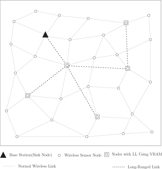
Figure 7.11. An example SWWSN created by the VRAM model where only about 15% of all sensor nodes (five nodes) with high BC values are chosen for VRAM-based LL formation

In Step I, the BS gathers the network topology of the sensor nodes. Since the topology can be large, this information cannot be easily gathered and used by individual sensor node. Therefore, the BS gathers the network topology and proceeds with the rest of the process in a centralized manner.

Once the topology of WSN is obtained, in Step II, the BS estimates the BC value of all the sensor nodes in the network (see Figure 7.11). BC value for a given node X can be obtained by estimating the ratio of the shortest paths in which X is involved to that of the total number of shortest paths between all source-destination pairs. Information about how to calculate BC can be found in Section 3.2.6.

To create LLs it is required to identify a limited number of nodes as a set, LLNodeSet. The exact number of nodes selected in the LLNodeSet is a design parameter that can be chosen by the network engineer based on the network topology, number of nodes, and the reliability/robustness required for the network. Empirical estimation suggests a choice of 10% of the number WSN nodes in the LLNodeSet to create LLs.

The estimation of BC can be carried out in the traditional approach as discussed in Section 3.2.6 or using a simplified approximation approach, suggested as part of the VRAM-SWWSN, called neighbor-avoiding walk (NAW). In NAW, a walker is assumed to start from the BS and visits nodes in the WSN. In the node visiting process, the walker avoids previously visited nodes as well as the neighbors of previously visited nodes while making a decision to visit the next node. Such an approach helps efficient calculation of the BC values at the cost of introducing approximations in the BC values estimated.

In Step III, once the LLNodeSet membership is chosen based on the high BC values in the WSN, they can be instructed to form LLs by adapting the modulation rates to achieve longer ranges (see Figure 7.11). For example, a radio interface operating at 64-point constellation quadrature amplitude modulation (64QAM) can be adapted to operate in 16-point constellation QAM (16QAM) in order to obtain an increased transmission range, given similar transmit power and environmental conditions. Approximate range for a 16QAM radio interface can be obtained as follows:

where R₁₆ and R₆₄ represent the transmission ranges obtained when using 16QAM and 64QAM, respectively, under similar transmission power and identical environmental conditions. It can be seen that approximately 36% higher transmission range can be achieved by adapting the modulation rate from 64QAM to 16QAM. Further increase in the range can be achieved by lowering the modulation rate.

Disadvantages of the VRAM-SWWSN approach include (i) the estimation of BC values for an N node WSN can take an asymptotic time complexity of ?(N2logN) which requires significant computing time for a large WSN, (ii) the use of NAW can result in suboptimal BC estimate, and (iii) the use of radios with rate adaptation capability increases the cost of sensor nodes.

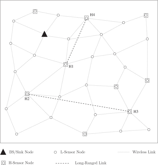
Figure 7.12. An example SWWSN created by degree-based LL addition where the H-sensor nodes with highest neighbor degree are chosen for LL addition

The major disadvantage of degree-based LL addition is that (i) in high assortativity networks, the addition of LLs may not be significant in APL reduction. That is due to the fact that the highdegree nodes are potentially closely located at certain specific regions of the network where addition of many LLs among the closely located nodes may not make significant improvement in APLB. Another disadvantage is that (ii) in a network with many high-degree nodes, the degree-based LL addition becomes ineffective as the solution reduces to a random LL addition method.

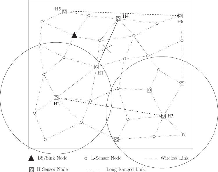
Figure 7.13. An example SWWSN created by inhibition distance-based LL addition where a minimal distance is maintained between any two LLs

Disadvantages of ID-SWWSNs include the following: (i) In order to estimate the inhibition distance, either geographic distance between nodes or global network topology is required. (ii) The number of LLs that can be added may be limited in a small or medium scale SWWSN. Further, (iii) the optimal value of inhibition distance is not known.

• Step I—Construct a narrow search space between WSN nodes and the BS.

• Step II—Identify WSN nodes that can form LLs within the narrow search space.

• Step III—Rotate the role of LL node formation among the nodes in the narrow search space in order to uniformly consume energy.

In Step I, a narrow physical space is identified for a WSN node and the BS by estimating a line formed by the WSN node and the BS. Consider the node marked i in Figure 7.14. This line, shown in Figure 7.14 as Line-1, can be estimated by using the location coordinates of the node i and the BS. The location information of the BS can be received by the WSN nodes through periodic packet updates, or it can be considered as the origin with coordinates (0, 0). Line-1 can be expressed as y = m × x; therefore, the gradient of Line-1 can be obtained as m=yixj where x_i and y_i are the x and y coordinates of Line-1 at any point i. In parallel to Line-1, and at distance D, two more lines, for example, Line-2 and Line-3 in Figure 7.14, are identified. The area between Line-2 and Line-3 within the network field region is identified as the narrow search space. Figure 7.14 shows the narrow space region formed between a node i and the BS.

Figure 7.14. An example SWWSN created by HgSWWSN model

In Step II, a subset of WSN nodes, located in the narrow search space, is identified by an efficient approach. The efficiency is achieved because every node can use local information, its local location coordinates, and information on the Line-1 coordinates to determine its presence within the narrow search space. That is, for any given WSN node k, located at coordinates (x_k, y_k) with as minimal information as the equation for Line-1, can estimate the distance d from the node to Line-1 as d=|yk−mxk|1+m2. Node k also checks whether d < D in order to determine its presence within the narrow search space. This method of determination of the existence of nodes within the narrow search space requires very small communication bandwidth because it does not require transmission of large volume of location information packets by the nodes.

Step III deals with the creation of LLs or selection of nodes within the narrow search space to work as end points for LLs. A node can be selected as an LL end point, based on a cluster-head election approach, with an end point LL addition probability parameter p [136]. The selection of LL end points is done only for a specific time duration. For example, a WSN node, k, can be selected as an LL end point to play the role of LL with probability time duration T_k where

and R represents the number of the round of operation. This relationship is used for nodes that have not been operating an LL in the last 1p rounds. Otherwise, the node does not form an LL in the current time slot. Further, note that the WSN node selected as an LL end point operates only for a time duration proportional to T_k. Such a distributed LL addition and deletion approach makes sure that each WSN node takes part in LL creation and operates only for a limited time at higher transmission powers.

Consider an example where the LL addition probability p = 0.25. For the 25^th round, the time slot value can be obtained as proportional to 0.33 units of time. That is, for a duration of 0.33 fraction of unit time, a node acts as an LL node. If the probability value is modified to p = 0.1, then in the same 25^th round, the LL formation fraction of time is about 0.2.

Therefore, at any given time, if there are N nodes in the narrow search space, the area may have about T_k × N LL end points. These LL end points operate their radios at higher transmission power to provide the necessary LLs to achieve shortcut paths. After the current round, another subset of nodes will operate as LL end points. The choice of a node to act as an LL end point can be estimated in a fully distributed way by using Equation (7.6.12).

The major disadvantages of this approach is (i) the requirement that every node needs to form LLs, which result in expensive nodes. Moreover, (ii) optimal value for p is not known.

The network model for SWWSN using wired LLs considers placement of LLs in a specific manner such that the routing of packets can utilize the locations of LLs. One end of the wired LLs is placed at distance closer (typically one hop) to the BS in the WSN. The other ends of the LLs are placed at the circumference of an imaginary circle whose center is located at the BS. The radius of the imaginary circle is taken as the length of the wired LL. Edges of the LLs that are located on the imaginary circle can be placed approximately equidistant so that the wired LLs can be utilized in a uniform manner. Note further that the imaginary circle may not be entirely covered in the WSN field, as shown in Figure 7.15. In the figure, the points marked by p, q, and r are the wired LL end points on the imaginary circle. The other end points of LLs are one hop away from the center of the LLs (i.e., the BS).

Figure 7.15. An example of wired LL based SWWSN

Figure 7.16 shows the routing approach used in wired SWWSN. Imagine a new LL is added between nodes w_i1 and w_i2, as shown in the figure. The cost of routing from WSN node B to the BS can be estimated based on the cost of the route using the LL or without using the LL. While the cost of path between node A to the BS is d(A, BS), the cost of the path through the LL is Cost(A, w_i1)+ Cost(LL) + Cost(w_i2, BS). The path cost taken for the APLB estimation is the lower of the available two paths. Thus, the path cost between node A and the BS can be

Figure 7.16. Routing in wired LL based SWWSN

In situations where the LL is directly connected to the BS, the cost of path through the LL can be obtained as Cost(A, w_i1)+ Cost(LL).

It can be observed from the simulation studies that close to 70% reduction in APLB can be achieved for cases where the BS is located at the center of the network.

The major disadvantages of this approach are that (i) use of wired LLs requires significant amount of time for planning and deployment, (ii) very long wired LLs may need additional relay devices with additional power sources, (iii) cost of wired links can be high, resulting in expensive network deployment, and (iv) it is not suitable for WSNs with mobility.

• One of the biggest challenges in the formation of LLs in an SWWSN is the hardware resource constraints of a WSN node. Since WSN nodes are of limited battery energy and consist of short-range radio and minimal computing power, realizing LLs by increasing transmission power is very challenging. One approach that is worth research investigation in SWWSNs is the possibility of forming distributed LLs. Distributed LLs can be formed by synchronized transmission operation of short-range radios of multiple WSN nodes such that their simultaneous operation can create a long-ranged communication link which can function as an LL. Such deployment can be considered as a dynamic LL, created for a short while, to relay a selected subset of the packets from one part of the network to another.

• Another open research problem in an SWWSN is the formation of dynamic LLs by using mobile relay nodes (data mules) that are more capable than the WSN nodes. For example, the data mule formed by a UAV can also create a trajectory of flight which can resemble an LL. Another possibility for creating a dynamic LL is to use the resource-rich radio transceiver of the UAV. The use of data mules as LLs in the context of SWWSNs is an interesting research area.

• Data fusion in WSNs refers to the special ways of data processing such that the overall data required to be transferred can be reduced while the information to be sensed can be retained. While in traditional WSNs, there exist many studies on data fusion techniques, in the context of SWWSNs, data fusion can be studied for improving performance while using the presence of LLs. The nodes with LLs are of particular interest in employing data fusion for improving the effectiveness of data fusion as well as for saving bandwidth resources.

• Similar to data fusion in SWWSNs, another interesting open problem is in the application of network coding in the presence of LLs in SWWSNs. Network coding is a recently introduced networking technique where the raw data is encoded as well as decoded in a network-wide manner by using algebraic algorithms so that the throughput can be improved, delay can be reduced, and the network robustness can be enhanced. While in traditional wired as well as wireless networks, there have been many existing works on network coding, in SWWSNs applying network coding can utilize the presence of LLs that aggregate data in a more significant manner than the other nodes. Therefore, new network coding algorithms can be developed for SWWSNs.

• In the context of string topology SWWSN, optimal energy-efficient LL addition was studied for only one to two LLs. Therefore, a generalized algorithm for adding k LLs in such a network is an open research problem.

• Similar to the above mentioned open problem, the optimal energy efficient LL addition is studied only for string topology SWWSNs which is a 1-D network. In the case of 2-D or 3-D networks, energy-efficient optimal LL addition remains an open research problem under the following cases: (i) 2-D and 3-D regular grid topology networks and (ii) 2-D and 3-D arbitrary topology networks. Another interesting open problem is in the existence or identification of anchor points in 2-D and 3-D SWWSNs.

• While there exist some routing protocols for SWWMNs, they are not suitable for efficient operation in SWWSNs. Therefore, routing protocols provide opportunities for research in SWWSNs, particularly with the emphasis on designing efficient routing protocols that consider the presence of LLs, possibility of network coding over LLs, and data fusion.

• In SWWSNs, the LLs carry aggregated traffic from many WSN nodes, and as a result, they can face higher traffic load. Therefore, link-level packet aggregation as well as data compression can be beneficial in efficient utilization of the LL bandwidth.

• Compressed sensing is an approach to avoid redundancy in WSNs, thereby improving the efficiency of resource management in WSNs. Therefore, when transforming WSNs to SWWSNs, compressive sensing can be very useful in determining the locations of LLs. Novel LL addition strategies can be developed by following compressive sensing techniques with energy efficiency considerations.

• A set of interesting open research problems emerge in SWWSNs when we consider software defined radio (SDR)-based radio interfaces. SDRs allow programmability of radios, thereby modifying the modulation techniques, transmission ranges, data rates achieved, as well as energy consumed. While today SDRs consume significant amounts of computing power and energy resources, advancement in the area of SDRs can result in using SDRs in highly constrained networks such as WSNs. When SDRs are used in sensor nodes, every sensor node may obtain LL capability, thereby enabling the possibility of a potentially large number of nodes with LL capability. One of the important issues in using long-range transmissions is the possibility of high interference, which will bring down the achievable network capacity. To manage the interferences, programmability of the SDRs can be utilized. Such an SDR-based SWWSN environment offers a rich set of open research issues including the following: (i) the possibility of variable transmission range LLs and the study of impact of variable transmission range LLs, (ii) the optimal number of LLs and their transmission range distribution, (iii) interference-aware LL usage algorithms, and (iv) optimal locations of LLs with variable transmission range.

• The Braess paradox [127] is known for describing the situation where a new link addition in a network may worsen the network performance. For example, a new road addition to improve the travel time and reduce the traffic congestion in an already congested road network may further worsen the travel time and traffic congestion if all the commuters prefer the new road. The following open problems exist in this direction: (i) the possibility and conditions of existence of the Braess paradox in SWWSNs, (ii) the conditions of edge-weight requirements that may avoid the possibility of existence of the Braess paradox in a SWWSN, and (iii) the design of routing protocols that can avoid the Braess paradox situation in SWWSNs.

• Interference between wireless LLs and normal links can be a significant problem in SWWSNs. Existing models are insufficient to study the impact of interference between LLs and normal links. Open research issues include creating accurate simulation or analytical models of SWWSNs for studying the interference issues under the following two cases: (i) when LLs and normal links share the same channel and (ii) when LLs and normal links use separate channels. Further, channel allocation or transmission scheduling algorithms that can minimize the interference between LLs and normal links are also interesting open research issues.

1. Conduct a survey of technical specifications of a number of WSN nodes and prepare a comparison table on the following items: form factor of the nodes; energy used by the nodes during transmission, reception, sleep, and idle modes; transmission range; data rate; number of radio interfaces; and other major technical specifications. Judge for yourself on the sensors with radio transceivers that can be used for forming LLs. Prepare a short list of WSN nodes that can be used for formation of SWWSNs.

2. In a SWWSN, the low-power sensor nodes usually transmit at a transmit power such that the transmission range is 10 meters. The terrain where the network is deployed has been found to have a path loss exponent of 2.2. In order to increase the transmission range of selected sensor nodes to form LLs, a radio frequency (RF) amplifier can be connected to the output of the transmitter. The range required for the LL is estimated as 40 meters. Estimate the percentage increase in transmit power that will be consumed due to the use of the RF amplifier.

3. Write a computer program for simulating a random model for SWWSN for a WSN area of 1 square kilometer. Assume the sensors have two network interfaces, one short-range (10m) and another long-range (50m). Use uniform distribution of WSN nodes in the field. Also assume that the connectivity among the WSN nodes with LL is decided based on the Euclidean distance between sensor nodes and the range of the LL. Assume that the sensed data traffic flow is from the WSN nodes to the BS located at corner of the WSN field. Average your observations for at least 10 different random positions of the WSN nodes and link formations. Estimate the following:

(a) Average number of LLs formed in the network.

(b) Average number of WSN nodes that are one hop away from a WSN node with LL.

(c) Average path length from WSN nodes to the BS with and without the LLs.

4. Consider an N-node string topology WSN transformed to an SWWSN by adding one LL between the BS and the node at location N2 . After the transformation is carried out, the APLB is reduced to less than N5 . While the location of LL addition halves the WSN, the reduction in APLB is much more than its proportion. What is the likely reason for the nonlinear decrease in the APLB?

5. In the string topology SWWSN shown in Figure 7.5, estimate the traffic load that needs to be carried by the LL when the LL is connected between the BS and the WSN node at location 0.6N. Assume the routing protocol used by the SWWSN nodes is shortest path routing and each sensor node generates an approximate traffic of k bits per second.

6. For the above problem, estimate the APLB reduction factor due to the transformation to an SWWSN. What is the impact on APLB when you add one more LL to the SWWSN between locations 0.3N and BS?

7. In a string topology SWWSN with one LL, prove that the optimal LL addition for achieving minimal APLB is made between the BS and the node at fractional location 0.6.

8. Write a computer program to simulate a large string topology SWWSN with 1000 nodes or larger where nodes are uniformly spaced at distances such as 20 meters. Simulate LL additions among all node pairs such that location for one LL that results in the lowest APLB can be identified. Note the locations for adding 1, 2, 5, and 10 LLs in sequence by minimizing APLB at each stage. Now consider the limitation on the transmission range of the links by eliminating LL possibilities beyond 100 meters. With the LL constraint, estimate the locations for adding 1, 2, 5, and 10 LLs in sequence. Make your own observations on the impact of length constraints of the LLs.

9. Write a computer program to simulate a grid topology network of very large size (∼1024 nodes). Using this simulated topology, estimate the nodes where LLs can be connected to achieve the minimum APLB in the network after the LL addition, when the BS is located at a corner of the grid topology. Make your own observations on the location and repeat the experiment to add a second LL after addition of the first.

10. Consider a random model–based SWWSN with N_L L-sensors and N_H H-sensors where the probability of adding LLs between H-sensors is taken as p. What is the mean number of LLs that can exist in the network? Also what is the probability of having the H-sensors connected by LLs to form a connected subgraph?

11. In a NW-SWWSN, the transmission range of the long-range transmitter of H-sensor nodes is about 250 meters. The highest LL addition probability is set to 0.8. Estimate the LL addition probability, p, for the structural parameters 2 and 3 for a given link between two nodes separated at distance 20 meters. Also estimate the probability of LL addition between two nodes separated by a distance 300 meters.

12. Consider a DRM-SWWSN where there are N nodes spread across an area of Am² in a uniform distributed manner. Assume that all nodes have H-sensor capability. For a directed angle of θ = 30 degrees, estimate the mean number of members in the DNT given the probability p = 0.2. What are the impacts of having a very small number of members in the DNT?

13. In a VRAM-SWWSN, assume the normal transmission range of the radio interface is estimated as 100 meters when using a modulation rate of 64QAM. For creating LLs, rate adaptation is employed in a dynamic manner to two lower modulation rates by adapting to the following two levels: (a) 32 QAM and (b) 8 QAM. Assume the path loss exponent is 2 and the transmission power is fixed. Estimate the transmission range of the LLs when operating at the two lower rates. Suggest a method to utilize the two LL ranges in a way to achieve energy efficiency in the SWWSN.

14. Assuming a centralized algorithm for implementing the degree-based SWWSN, estimate the asymptotic time complexity for adding k LLs in a sensor network of N nodes. Also compare the estimated time complexity of degree-based SWWSN to the time complexity of ID-SWWSN where the inhibition-distance is taken as equal to twice that of the length of normal links.

15. Consider HgSWWSN where the narrow search space in which the nodes form an LL is limited to 1km × 0.1km. The node density of sensors in the entire sensor network field is about 500 sensors per square kilometer. If the probability of a WSN node forming an LL is about 0.1, estimate the following: (a) the fraction of time a given node operates its LL in the first round of operation and (b) the number of WSN nodes with LL present in the narrow search space.

16. In a wired LL–based WSN that spans a radius of 1000 meters, estimate the optimal length, L, of LLs that need to be used for minimizing the APLB. Assume all the LLs are of constant length and are deployed from BS to a circle of radius L.

17. Simulate an SWWSN environment where the BS is located at the center of the network and the network is in a circular shape with radius R meters. Assume a large number of wired LLs are employed where the LLs are added from the BS to a circle at distance L from the center of the network. Nodes are distributed uniformly in the network area. (a) Estimate the APLB with and without the LLs and plot the APLB variation against the number of LLs added. (b) Locate the BS at the periphery of the network and repeat (a). (c) Simulate and develop an empirical model for optimal LL length for LLs where the length may vary randomly within a range.

18. Conduct a literature survey of WSNs with at least five different real-world application scenarios. Categorize the identified application scenarios based on the suitability for transformation to SWWSNs. Also identify the most suitable transformation mechanism among existing techniques discussed in this chapter.

19. Consider an SWWSN with arbitrary topology with N nodes. Each node has a certain fixed transmission range t_x. Develop an algorithm for adding LLs in the network such that both energy consumption and end-to-end delay can be optimized. Assume suitable transmission range for the LLs.

20. Create a simulation model for SWWSN using a widely used network simulator, such as Network Simulator 2 (NS2), with a total of N nodes out of which M nodes have LL capability. Create an appropriate routing protocol for the SWWSN. Assume that the normal links and LLs use the same or different transmission channels. LLs use directional radios compared to the omnidirectional radios used by the normal links. Using the simulation model, conduct experiments to gather information on the impact of LLs sharing the same channel as the normal links.

1. The base station is also known as sink node (SiN) or monitoring station (MS). In this book, we use these terms interchangeably.

2. Note that an LL is also referred to as a shortcut link or a new link. In this textbook, we use these terms interchangeably.

3. A detailed technical discussion on Iridium 9602 can be found in [128].