In the planar analysis, the rotation of the rigid body can be described using one coordinate, such that the angular velocity of the body is defined as the time derivative of this orientation coordinate. Furthermore, the order of the finite rotation is commutative since the body rotation is about the same axis. Two consecutive rotations can be added and the sequence of performing these rotations is immaterial. One of the principal differences between the planar and the spatial kinematics is due to the complexity of defining the orientation of a body in a three-dimensional space. In the spatial analysis, the unconstrained motion of a rigid body is described using six coordinates; three coordinates describe the translation of a reference point on the body and three coordinates define the body orientation. The order of the finite rotation in the spatial analysis is not commutative and, consequently, the sequence of performing the rotations must be taken into consideration. Moreover, the angular velocities of a rigid body are not the time derivatives of a set of orientation coordinates. These angular velocities, however, can be expressed in terms of a selected set of orientation coordinates and their time derivatives.
In this chapter, methods for describing the orientation of rigid bodies in space are presented. The configuration of the rigid body in a multibody system is described using a set of generalized coordinates that define the global position vector of a reference point on the body as well as the body orientation. As in the planar analysis, coordinate transformations are defined in terms of the generalized orientation coordinates. The relationships between the angular velocity vectors and the time derivatives of the generalized orientation coordinates are developed and used to define the absolute velocity and acceleration vectors of an arbitrary point on the rigid body. These kinematic relationships are then used to develop the dynamic equations of motion of multibody systems in terms of the system-generalized coordinates. As it is shown in the analysis presented in this chapter, the equations that describe the motion of a rigid body in three-dimensional space are quite complex as compared to the equations of the planar motion. Derivation of the dynamic equations of motion and definition of the mass matrix of spatial rigid body systems are presented and the simplifications in the dynamic relationships when the reference point is selected to be the body center of mass are discussed. This special case leads to the formulation of the Newton-Euler equations, in which there is no inertia coupling between the translation and rotation of the rigid body. The application of the augmented formulation and recursive methods to the dynamics of spatial multibody systems consisting of interconnected rigid bodies is also demonstrated in this chapter.
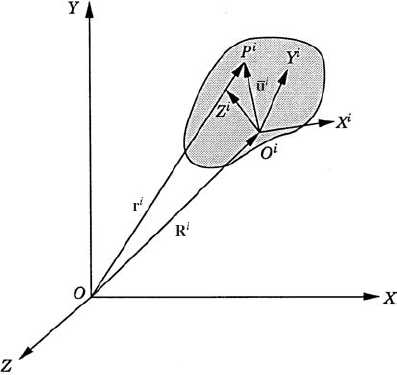
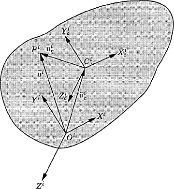
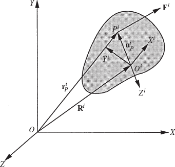
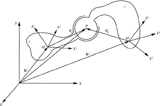
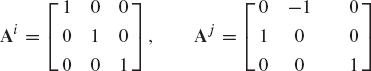
In the three-dimensional analysis, the unconstrained motion of a rigid body is described using six independent coordinates; three independent coordinates describe the translation of the body and three independent coordinates define its orientation. The translational motion of the rigid body can be defined by the displacement of a selected reference point that is fixed in the rigid body. As shown in Fig. 1, which depicts a rigid body i in the three-dimensional space, the global position vector of an arbitrary point on the body can be written as
where Ri is the global position vector of the origin of the body reference Xi YiZi, Ai is the transformation matrix from the body coordinate system to the global XYZ coordinate system, and
and
In the case of pure translational motion, the orientation of the body does not change, and consequently, all the points on the rigid body move with equal velocities. On the other hand, if the reference point is fixed, the body does not have the freedom to translate and the remaining degrees of freedom are rotational.
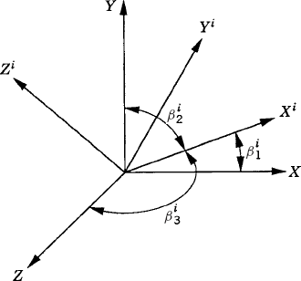
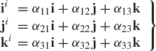
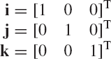
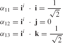
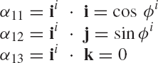
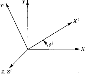
In this section, a method for determining the transformation matrix Ai of Eq. 1 is presented. This matrix defines the orientation of the body coordinate system XiYiZi with respect to the coordinate system XYZ. Figure 2 shows the coordinate system XiYiZi of body i. The orientation of this coordinate system in the XYZ system can be described using the method of the direction cosines. Let ii, ji, and ki be unit vectors along the Xi, Yi, and Zi axes, respectively, and let i, j, and k be unit vectors along the axes X, Y, and Z, respectively. Let βi1 be the angle between the Xi and X axes, βi2 be the angle between Xi and Y axes, and βi3 be the angle between Xi and Z axes. The components of the unit vector ii along the X, Y, and Z axes are given, respectively, by
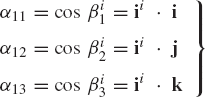
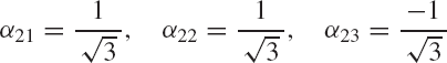
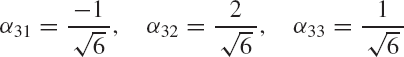
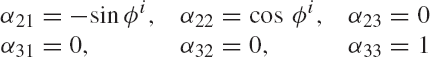
where α11, α12, and α13 are the direction cosines of the Xi axis with respect to the X, Y, and Z axes, respectively. In a similar manner, the direction cosines α21, α22, and α23 of the axis Yi, and the direction cosines α31, α32, and α33 of the axis Zi, can be defined as
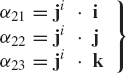
and
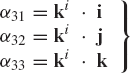
Since the direction cosines αij represent the components of the unit vectors ii, ji, and ki along the axes X, Y, and Z, one has
Let us now consider the vector ui whose components in the body i coordinate system are denoted as
or
Substituting Eq. 7 into Eq. 8, one obtains
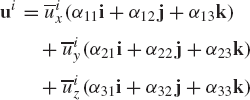
which leads to
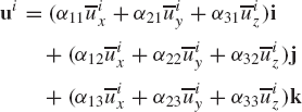
By comparing Eqs. 9 and 10, one concludes
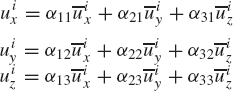
That is, the relationship between the coordinates of the vector ui in the XYZ coordinate system, and its coordinates in the XiYiZi coordinate system, can be written in the following matrix form
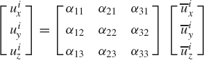
In order to distinguish between the two different representations of the vector ui, this vector will be denoted as
and
Using this notation, Eq. 11 can be rewritten as
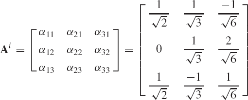
where Ai is recognized as the transformation matrix defined in terms of the direction cosines αij, i, j = 1, 2, 3 as
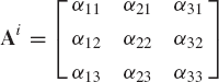
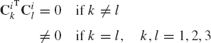
The transformation matrix of Eq. 15 is expressed in terms of nine parameters αij, i, j = 1, 2, 3. The nine direction cosines αij are not totally independent because only three independent parameters are sufficient to describe the orientation of a rigid body in space. Since the direction cosines represent the components of three orthogonal unit vectors, they are related by the six algebraic equations
where δkl is the Kronecker delta defined as
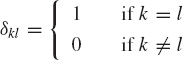
Because of the six algebraic relationships of Eq. 16, there are only three independent components among the elements of the transformation matrix Ai.
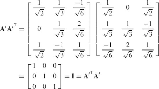
An important property of the transformation matrix is the orthogonality, that is
where I is the 3 × 3 identity matrix. The orthogonality of the transformation matrix can be verified by direct matrix multiplication and the use of the identity of Eq. 16. The relationship of Eq. 18 remains valid regardless of the set of coordinates used to describe the orientation of the body in the three-dimensional space.
Example 7.1
If the axes Xi, Yi, and Zi of the coordinate system of body i are defined in the coordinate system XYZ by the vector [1.0 0.0 1.0]T, [1.0 1.0 −1.0]T, and [−1.0 2.0 1.0]T, obtain the transformation matrix that defines the orientation of the coordinate system XiYiZi with respect to the system XYZ.
Solution. The unit vectors ii, ji, and ki along the axes Xi, Yi, and Zi are
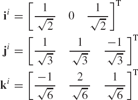
The vectors i, j, and k are
It follows that
Similarly,
and
The transformation matrix Ai that defines the orientation of the coordinate system XiYiZi with respect to the coordinate system XYZ is
Note that
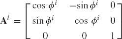
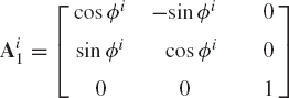
We now consider the case of simple finite rotations of the coordinate system XiYiZi about the axes of the coordinate system XYZ. Consider the case in which the axes of the two coordinate systems are initially parallel and the origins of the two systems coincide. First we consider the rotation of the coordinate system XiYiZi about the Z axis by an angle ϕi. As shown in Fig. 3, as a result of this finite rotation
Similarly, one can show that the other direction cosines are
It follows that the transformation matrix that defines the orientation of the coordinate system XiYiZi as the result of a rotation ϕi about the Z axis is given by
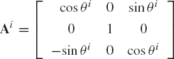
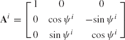
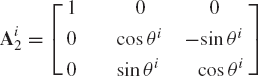
The use of a similar procedure shows that if the coordinate system XiYiZi rotates an angle θi about the Y axis, the transformation matrix is
and in the case of a rotation ψi about the X axis, the resulting transformation matrix is
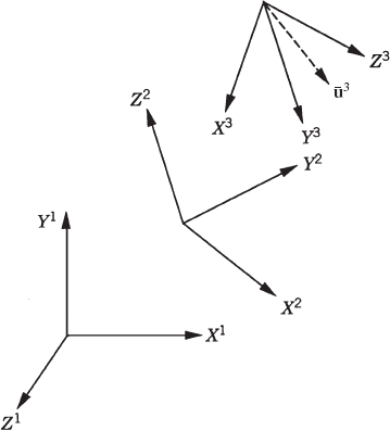
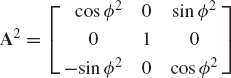
As demonstrated in Chapter 1, the order of the finite rotation is not commutative. An exception to this rule occurs only when the axes of rotation are parallel. Consider the case of three coordinate systems X1Y1Z1, X2Y2Z2, and X3Y3Z3. As shown in Fig. 4, these three coordinate systems have different orientations. Let A32 be the transformation matrix that defines the orientation of the coordinate system X3Y3Z3 with respect to the coordinate system X2Y2Z2, and let A21 be the transformation matrix that defines the orientation of the coordinate system X2Y2Z2 with respect to the coordinate system X1Y1Z1. Let
The components of the vector u2 can be defined in the coordinate system X1Y1Z1 by the vector u1, where
Substituting Eq. 22 into Eq. 23, the vector u1 can be expressed in terms of the original vector
which can be written as
where, in this case, the transformation matrix A31 that defines the orientation of the coordinate system X3Y3Z3 with respect to the coordinate system X1Y1Z1 is given by
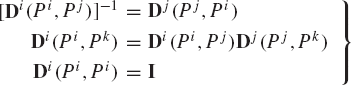
Similarly, in the case of n coordinate systems, one has
where Aij is the transformation matrix that defines the orientation of the ith coordinate system with respect to the jth coordinate system. Note that in general
as previously demonstrated.
Example 7.2
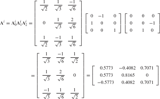
In the initial configuration, the axes Xi, Yi, and Zi of the coordinate system of body i are defined in the XYZ coordinate system by the vectors [1.0 0.0 1.0]T, [1.0 1.0 −1.0]T, and [−1.0 2.0 1.0]T, respectively. The body then rotates an angle θi1 = 90° about its Zi axis followed by a rotation θi2 = 90° about its Xi axis. Determine the transformation matrix that defines the orientation of the body i in the XYZ coordinate system as a result of the successive rotations. If
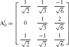
Solution. In the initial configuration, the method of the direction cosines can be used to determine the transformation Ai0 that defines the orientation of the body before the rotations θi1 and θi2. It was shown in Example 1 that this transformation matrix is
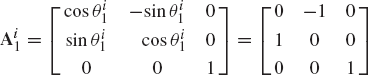
As a result of the rotation θi1, the body occupies a new position. The orientation of the body as a result of this rotation is defined with respect to the initial configuration by the matrix Ai1 defined as
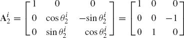
Since the second rotation θi2 is about the Xi axis, the matrix Ai2 is given by
The final orientation of the body is defined by the matrix Ai given by
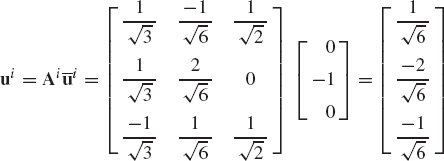
The components of the vector
The direction cosines are rarely used in describing the three-dimensional rotations of multibody systems. Among the most widely used parameters for describing the orientation are the three independent Euler angles. Several different sets of Euler angles are in common use in the analysis of mechanical and aerospace systems. In this section, the most widely used Euler angles are defined and the transformation matrix in terms of them is developed.
Euler angles involve three successive rotations about three axes that are not, in general, perpendicular. By performing these three successive rotations in the proper sequence, a coordinate system can reach any orientation. Consider the coordinate systems XYZ and XiYiZi, which initially coincide. The sequence starts as shown in Fig. 5, by rotating the system XiYiZi an angle ϕi about the Z axis. Since ϕi is a rotation about the Z axis, the transformation matrix resulting from this rotation is given by
The coordinate system XiYiZi is then rotated an angle θi about the current Xi axis, which at the current position is called the line of nodes. The change in the orientation of the coordinate system XiYiZi as a result of the rotation θi is described using the matrix
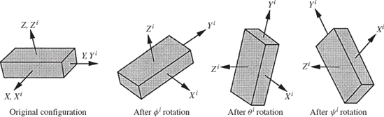
Finally, the coordinate system XiYiZi is rotated an angle ψi about the current Zi axis. The change in the orientation of the system XiYiZi as a result of this rotation is given by
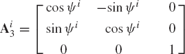
Using the transformation matrices Ai1, Ai2, and Ai3 given, respectively, by Eqs. 28, 29, and 30, the final orientation of the coordinate system XiYiZi can be defined in the system XYZ by the transformation matrix Ai given by
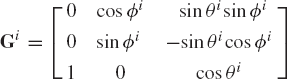
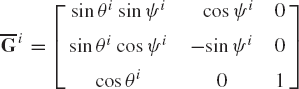
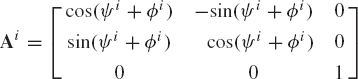
This equation can be used to define the matrix Ai in terms of the angles ϕi, θi, and ψi as

The three angles ϕi, θi, and ψi are called the Euler angles. The orientation of any rigid body in space can be obtained by performing these three independent successive rotations.
In the discussion presented in this section, we considered the sequence of rotations about the Zi, Xi, and Zi axes. Other sequences that are also used to define Euler angles are rotations about Zi, Yi, and Xi, or rotations about Zi, Yi, and Zi. The use of these sequences leads to transformation matrices that are different from the one presented in this section. The procedure used to define the transformation matrix using these sequences, however, is the same as described in this section and is left to the reader as an exercise. There are also other sets of rotational coordinates that are often used to describe the orientations of rigid bodies in space. Among these coordinates are the four Euler parameters and the three independent Rodriguez parameters. These sets will be introduced in the following chapter.
Using the fact that the elements of the transformation matrix are the direction cosines of the axes Xi, Yi, and Zi, the nine direction cosines can be easily expressed in terms of Euler angles. For instance, the elements of the third column in the transformation matrix of Eq. 32 are the direction cosines of the Zi axis. These three direction cosines are functions of the angle ϕi since the rotation θi is about an axis whose direction cosines are defined by the unit vector
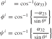
The quadrants where the angles lie are selected so as to ensure that all the remaining elements in the Euler angle transformation matrix are the same as the elements of the transformation matrix evaluated using the direction cosines.
The general displacement of a rigid body in space is the result of translational and rotational displacements. In this case, the global position vector of an arbitrary point on the body is given by Eq. 1, which is reproduced here:
where Ri is the global position vector of the origin of the body fixed coordinate system, Ai is the transformation matrix that defines the orientation of the body in the global coordinate system, and
The absolute velocity of an arbitrary point on the rigid body can be obtained by differentiating Eq. 33 with respect to time. This leads to
Since the transformation matrix is orthogonal, one has
which upon differentiation leads to
or
This equation implies that
A matrix that is equal to the negative of its transpose is a skew symmetric matrix. Therefore, Eq. 38 can be written as
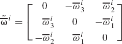
where ω~ i is a skew symmetric matrix that can be written as
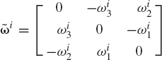
and ωi1, ωi2, and ωi3 are called the components of the angular velocity vector ωi, that is
Postmultiplying both sides of Eq. 39 by the matrix Ai and using the orthogonality of the transformation matrix, one obtains
Substituting this equation into Eq. 34 yields
which can also be written as
where
Using the cross product notation, Eq. 44 can be rewritten as
Example 7.3
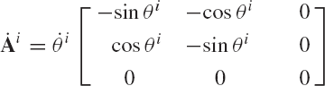
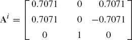
Consider the case in which the rigid body i rotates about the fixed Z axis. If the angle of rotation is denoted as θi, the transformation matrix is
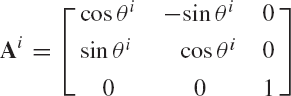
and
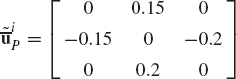
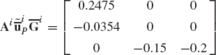
The skew-symmetric matrix ω~i of Eq. 39 is
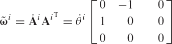
That is,
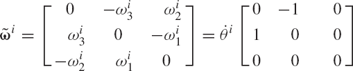
which defines the angular velocity vector ωi as
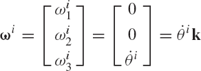
where k is a unit vector along the axis of rotation. The preceding equation, which is the familiar form of the angular velocity vector used in the planar analysis, is obtained here using the general development presented in this section.
Equation 39 defines the components of the angular velocity vector in the global coordinate system. The components of this vector can also be defined in the coordinate system of body i using the transformation
where
An alternative form for the absolute velocity vector of an arbitrary point on the rigid body can be obtained by using the vector
which, upon differentiation, leads to
This implies that the matrix
where
where
Premultiplying Eq. 50 with Ai and using the orthogonality of the transformation matrix, one obtains
Substituting this equation into Eq. 34, another form of the absolute velocity vector of an arbitrary point on the rigid body can be obtained as
The use of Eqs. 42 and 53 implies that
Example 7.4
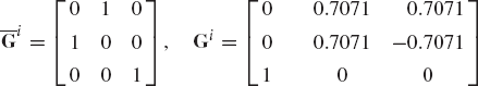
We again consider the case of simple rotation of a rigid body i about the fixed Z axis by an angle θi. The transformation matrix Ai and its time derivative
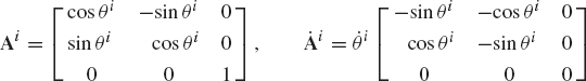
Using Eq. 50, one has
which defines the components of the absolute angular velocity vector in the body coordinate system as
Comparing these results with the results obtained in Example 3, we conclude in this special case of a simple rotation about a fixed axis that
are still in effect.
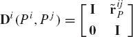
The transformation matrix that defines the orientation of an arbitrary body i can be expressed in terms of the transformation matrix that defines the orientation of another body j as
It follows that
where
holds (see Eqs. 55 and 56), where
which implies that
This equation states that the absolute angular velocity of body i is equal to the absolute angular velocity of body j plus the angular velocity of body i with respect to body j.
The equation of the absolute acceleration can be obtained by differentiating Eq. 34 with respect to time. This leads to
Differentiating Eq. 42 with respect to time, one obtains
Substituting Eq. 42 into Eq. 60, one obtains
where
Substituting Eq. 61 into Eq. 59, the absolute acceleration of an arbitrary point on the rigid body i can be written as
which, upon the use of Eq. 45 and the notation of the cross product, can be written as
where
Equation 64 can also be written in an alternative form as
in which
The kinematic and dynamic relationships of multibody mechanical systems can be formulated in terms of the angular velocity and acceleration vectors. The angular velocities, however, are not the time derivatives of a set of orientation coordinates and, therefore, they cannot be integrated to obtain the orientation coordinates. For this reason it is desirable to formulate the dynamic equations using the rotational coordinates such as Euler angles.
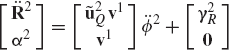
In order to achieve this objective, Eq. 46, which defines the absolute velocity vector of an arbitrary point on the rigid body i, is written as
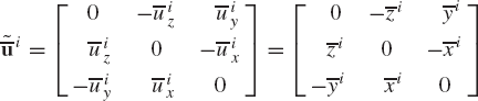
which can be written using the skew-symmetric matrix notation as
where u~i is the skew symmetric matrix
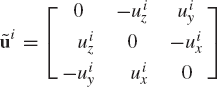
and uix, uiy, and uiz are the components of the vector ui.
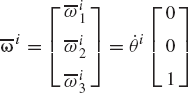
In Section 3, the transformation matrix that defines the orientation of body i was developed in terms of Euler angles. By using this transformation matrix and the identity of Eq. 39, the angular velocity vector ωi defined in the global coordinate system can be expressed in terms of Euler angles and their time derivatives as
where θi is the set of Euler angles defined as
and
The columns of this matrix, which represent unit vectors along the axes about which the Euler angle rotations ϕi, θi, and ψi are performed, are vectors defined in the fixed coordinate system.
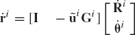
Substituting Eq. 70 into Eq. 68, the absolute velocity of an arbitrary point on the rigid body can be expressed in terms of Euler angles as
which can be written using matrix partitioning as
Similarly, the absolute acceleration of the arbitrary point on the rigid body can also be expressed in terms of the generalized orientation coordinates using Eq. 64, which can be written using the skew symmetric matrix notation as
Differentiating Eq. 70 with respect to time, one obtains
Substituting this equation into Eq. 74, the absolute acceleration vector
where aiv is a vector that absorbs terms which are quadratic in the velocities. This vector is defined as
The vector aiv absorbs the normal component of the acceleration as well as the portion of the tangential component that is quadratic in the velocities.
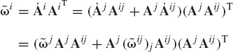
In the development of the kinematic equations presented in this section, the angular velocity and acceleration vectors defined in the global coordinate system are used. Another alternate approach to the formulation of the kinematic equations is to use the expressions of the angular velocity and acceleration vectors as defined in the body coordinate system. By following this procedure, one can show that
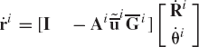
and

where
The matrix
where
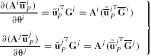
Using Eq. 47 or Eq. 50, it can be shown that the angular velocity vector
Equations 78 and 79 can be obtained directly from Eqs. 73b and 76 by using the identity
Recall that
Since
Comparing this equation with Eq. 75, one concludes that
Therefore, the quadratic velocity vector of Eq. 77 that also appears in Eq. 79 can be written in another form using the identity of Eq. 84 as
The fact that
It can be verified that the determinant of the matrix
which is a nonsingular orthogonal matrix whose inverse remains equal to its transpose. All Euler angle representations suffer from the singularity problem, which is encountered when two rotations occur about two axes that have the same orientation in space. In this case, the two Euler angles are not independent. A similar singularity problem is encountered when any known method that employs three parameters to describe the orientation of the rigid bodies in space is used. For this reason, the four Euler parameters are often used in the computer-aided analysis of the spatial motion of rigid bodies.
Equations 81 and 83 can be used to demonstrate that the components of the angular velocities are not exact differentials. For example, the use of these two equations defines
where
It is clear from these definitions that
which imply that
There are several methods for developing the dynamic equations of motion of the rigid bodies. In this chapter, the principle of virtual work in dynamics will be used to obtain the differential equations that govern the spatial motion of the rigid bodies. First, we develop in this section an expression for the virtual work of the generalized inertia forces.
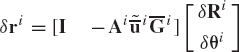
The virtual change in the position vector of an arbitrary point on the rigid body i is given by (see Eq. 78)
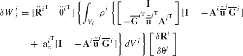
The virtual work of the inertia forces of the rigid body is
where ρi and Vi are, respectively, the mass density and volume of the rigid body i. Substituting Eqs. 79 and 92 into Eq. 93, one obtains
which can be written as
where qi is the vector of generalized coordinates of the rigid body i defined as
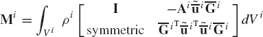
Mi is the symmetric mass matrix
and Qiv is the vector of the inertia forces that absorbs terms that are quadratic in the velocities. This vector is
In developing Eq. 95, the origin of the body coordinate system (reference point) is assumed to be an arbitrary point on the rigid body, and therefore, the mass matrix of Eq. 97 and the inertia force vector of Eq. 98 are presented in their most general form. Equations 97 and 98 can be simplified if the reference point is chosen to be the center of mass of the body, which is the case of a centroidal body coordinate system. The use of a centroidal body coordinate system is one of the basic assumptions used in developing the well-known Newton-Euler equations, which are discussed in later sections.
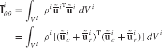
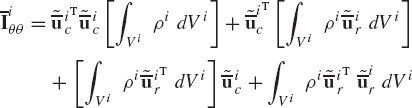
The symmetric mass matrix of the rigid body i defined by Eq. 97 can be written in the form
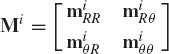
where mi is the total mass of the rigid body i, and
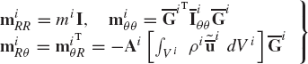
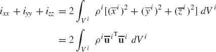
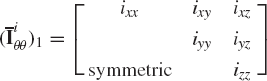
Using Eqs. 3, 82, and 101, the inertia tensor of the rigid body i can be written as
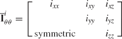
where the elements ixx, iyy, izz are called the moments of inertia and ixy, ixz, iyz are called the products of inertia. These elements are defined as
It is clear that the moments of inertia satisfy the following identity:
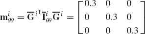
While the moments and products of inertia defined by Eq. 103 are constant since they are defined in the rigid body coordinate system, the matrix miθθ of Eq. 100 is a nonlinear matrix since it depends on the orientation coordinates of the rigid body. This matrix, upon the use of the identity of Eq. 80, can be written in an alternate form as
where
Note also that in the mass matrix of Eq. 99, there is a dynamic or inertia coupling between the translation and the rotation of the rigid body, and this coupling is represented by the off-diagonal nonlinear matrices, miRθ and miθR, which also depend on the orientation coordinates of the rigid body.
Example 7.5
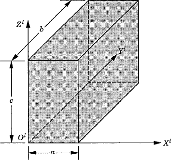
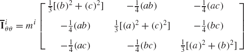
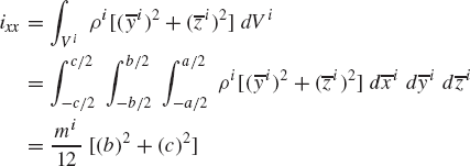
Obtain the components of the inertia tensor of the rectangular prism shown in Fig. 6 with respect to a coordinate system whose origin is located at one of the corners, as shown in the figure.
Solution. The elements of the inertia tensor can be evaluated using Eq. 103. For the rectangular prism shown in the figure,
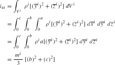
where mi is the total mass of the rectangular prism. Similarly, one can show that
The product of inertia ixy is
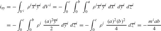
Similarly,
The inertia tensor of the rectangular prism defined in the coordinate system shown in the figure can be written as
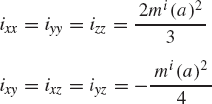
In the special case of a homogeneous cube, a = b = c, and the elements of the inertia tensor reduce to
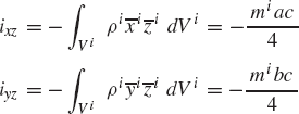
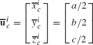
The elements of the inertia tensor given by Eq. 103 are defined in a coordinate system whose origin is attached to an arbitrary point on the rigid body. In this coordinate system, let
where
or
Since
and consequently,
The equation for the inertia tensor of the body becomes
where the fact that
was utilized, and
is the inertia tensor of the body defined in a centroidal XicYicZic coordinate system whose axes are parallel to the axes of the coordinate system XiYiZi as shown in Fig. 7. Equation 112 is called the parallel axis theorem, which states that the mass moments of inertia defined with respect to a noncentroidal coordinate system XiYiZi are equal to the mass moments of inertia defined with respect to a centroidal coordinate system XicYicZic plus the mass of the body times the square of the distances between the respective axes. These moments of inertia as well as the products of inertia can be expressed in terms of those defined with respect to the centroidal coordinate system as
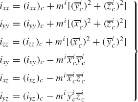
where (ixx)c, (iyy)c, (izz)c, (ixy)c, (ixz)c, and (iyz)c are the moments and products of inertia defined with respect to the center of mass, and
It is worth noting that since
or
which leads to
This equation defines the position vector of the center of mass with respect to the origin of the body coordinate system.
Example 7.6
For the rectangular prism of Example 5, obtain the elements of the inertia tensor defined with respect to a centroidal coordinate system whose axes are parallel to the axes of the coordinate system shown in Fig. 6.
Solution. It is clear in this simple example that the center of mass of the rectangular prism in the XiYiZi coordinate system is
This obvious result can also be obtained using the general equation
which, by assuming that the mass density ρi is constant, yields in this example
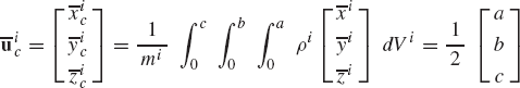
as expected.
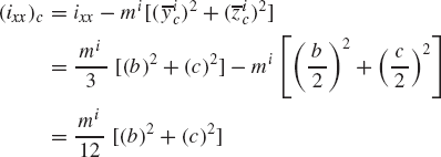
The element (ixx)c of the inertia tensor defined with respect to the centroidal coordinate system can be evaluated using the results obtained in Example 5 as
The product of inertia (ixy)c is
Using the results of the preceding example, one has
It can be also shown that
Thus,
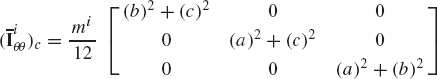
The results obtained in this example using the parallel axis theorem can also be obtained by attaching the origin of the body coordinate system XiYiZi to the center of mass and using Eq. 103. For example,
which is the same result obtained previously by the application of the parallel axis theorem.
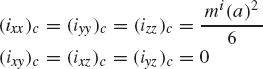
In the special case of a homogeneous cube, the moments and products of inertia reduce to
The parallel axis theorem shows the effect of the translation of the coordinate system on the definition of the moments and products of inertia. In order to define the relationship between two inertia tensors defined with respect to two body-fixed coordinate systems that differ in their orientation, let
Using this equation, it can be shown that the relationship between the inertia tensors defined in the two body-fixed coordinate systems can be written as
Using the orthogonality of the transformation matrix, and postmultiplying both sides of this equation by Ci, one obtains
It is possible to select the orientation of the body-fixed coordinate system Xi2Yi2Zi2 such that all the products of inertia are equal to zeros. In this special case, the inertia tensor
The principal axes and principal moments of inertia can be determined using Eq. 121. If Xi2, Yi2, and Zi2 are principal axes, the inertia tensor
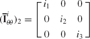
where i1, i2, and i3 are the principal moments of inertia. The inertia tensor
Now let Cik be the kth column of the transformation matrix Ci in Eq. 121. Equation 121 can, therefore, be written as
where I is the 3 × 3 identity matrix. Equation 124 is a system of homogeneous equations that can be solved for the vector Cik. This system has a nontrivial solution if and only if the coefficient matrix is singular. That is,
or
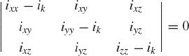
This determinant defines a cubic polynomial in ik. The roots of this polynomial define the principal moments of inertia ik, k = 1, 2, 3, and the principal directions Cik can be defined using Eq. 124. Since
Once Cik are determined, they can be used to determine unit vectors along the principal directions. These unit vectors define the vectors of the direction cosines, which form the columns of the transformation matrix Ci that defines the orientation of the coordinate system Xi2Yi2Zi2 with respect to the coordinate system Xi1Yi1Zi1. If two principal moments of inertia are equal, say i2 = i3≠i1, the direction of the principal axis associated with i1 is uniquely defined but any axis that lies in the plane whose normal is defined by Ci1 is a principal axis. In the case i1 = i2 = i3, any three mutually perpendicular axes form the principal directions. An example of this special case is the case of a sphere.
We note, in general, that in the case of repeated roots, the substitution of the repeated root in the coefficient matrix of Eq. 124 reduces the rank of this matrix by the number of the equal roots. This makes the dimension of the null space of the resulting coefficient matrix equal to the number of the repeated roots, ensuring that Eq. 124 has a number of independent solutions equal to the number of the repeated roots. These independent solutions define the principal directions.
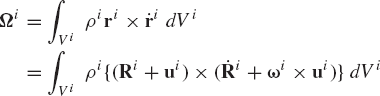
Using Eq. 98, the vector Qiv that absorbs terms that are quadratic in the velocities can be written as
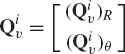
which upon the use of the expression for the vector aiv presented at the end of the preceding section yields
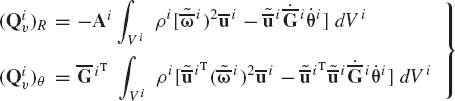
The vectors (Qiv)R and (Qiv)θ can be written as
and
where the definition of
The following vector and matrix identities can be verified
Using the last identity in the preceding equation, one has
The last two terms in this equation are identically equal to zero. Thus

Substituting this equation into Eq. 130, one obtains
The generalized external forces of the rigid body i can be defined using the expression of the virtual work. Examples of these forces are the gravity, spring, damping, friction, actuator forces, and motor torques. Examples of some of these forces which can be nonlinear functions of the system variables are presented in this section and the formulation of the generalized applied forces associated with the generalized coordinates of the spatial rigid body systems are discussed.
Let Fi be a force vector that acts at a point Pi on the rigid body i as shown in Fig. 8. This force vector is assumed to be defined in the global coordinate system. The virtual work of this force vector can be written as
where δriP can be obtained using Eq. 92 as
where
This equation can be obtained from Eq. 136 by using the identity of Eq. 84. Substituting Eq. 137 into Eq. 135, one obtains
or
in which
Equation 139 implies that a force that acts at an arbitrary point on the rigid body i is equipollent to another system defined at the reference point that consists of the same force and a set of generalized forces, defined by the second equation of Eq. 140, associated with the orientation coordinates of the body.
Since
Recall that uiP×Fi is the Cartesian moment resulting from the application of the force Fi, that is,
where Mia is the moment vector whose components are defined in the Cartesian coordinate system. Equation 141, therefore, defines the relationship between the generalized forces associated with the orientation coordinates and the Cartesian components of the moment as
One can also show that if the components of the moment vector are defined in the body coordinate system, one has
where
A special case occurs when the reference point lies on the line of action of the force Fi. In this special case, the vector uiP and the force Fi are parallel, and hence
It follows that Fiθ = 0. This equation and Eq. 140 imply that the effect of the force does not change if its point of application is moved to an arbitrary position along its line of action. For this reason, the force is considered as a sliding vector.
Example 7.7
A force vector Fi = [5.0 0.0 −3.0]T N is acting on body i whose orientation is defined by the Euler angles
The local position vector of the point of application of the force is
Using the absolute Cartesian coordinates and Euler angles as the generalized coordinates, define the generalized forces associated with the body-generalized coordinates.
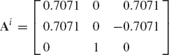
Solution. The transformation matrix that defines the orientation of the body is
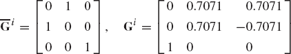
At the given configuration,
The virtual work of the force is
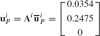
where
and
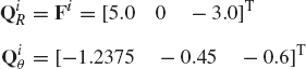
The generalized forces associated with the translation of the body reference are
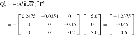
and the generalized forces associated with the orientation coordinates are
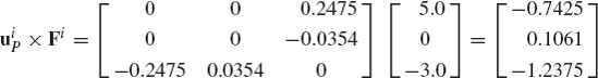
The generalized forces associated with the orientation coordinates can be defined using an alternative approach by first defining the Cartesian moment uiP×Fi, where
The Cartesian moment can then be defined as
The vector of generalized forces associated with the orientation coordinates is
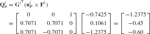
which is the same vector obtained previously.
If a rigid body i is subjected to a set of forces Fi1, Fi2, ..., Finf that act, respectively, at points whose position vectors are ri1, ri2, ..., rinf, and a set of moments Mi1, Mi2, ..., Minm, then the virtual work of these forces and moments can be written as
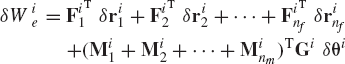
which upon the use of the relationship presented previously in this section yields
This equation can be written as
where (Qie)R and (Qie)θ are the vectors of generalized forces associated, respectively, with the generalized translation and orientation coordinates. These two vectors are defined as

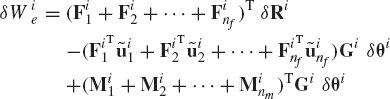
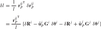
Figure 9 shows two bodies, body i and body j, connected by a spring-damper-actuator element. The attachment points of the spring-damper-actuator element on body i and body j are, respectively, Pi and Pj. The spring constant is k, the damping coefficient is c, and the actuator force acting along a line connecting points Pi and Pj is fa. Here, fa is a general actuator force that may depend on the system coordinates, on velocities, and possibly on time, and the coefficients k and c can also be nonlinear functions of the system variables. The underformed length of the spring is denoted as lo. The component of the spring-damper-actuator force along a line connecting points Pi and Pj can then be written as
where l is the current spring length. The first term on the right-hand side of Eq. 150 is the spring force, the second term is the damping force, and the third term is the actuator force. The virtual work of the force of Eq. 150 is
where
and rijP is the position vector of point Pi with respect to point Pj, that is,
where
which, upon using Eq. 152, yields
where
Let
be a unit vector along the line of action of the force Fs. Using the preceding equation and Eqs. 150 and 155, the virtual work of Eq. 151 takes the form
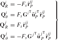
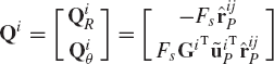
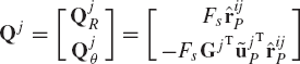
which can be written as
where the generalized forces QiR, Qiθ, QjR, and Qjθ are
The virtual work of Eq. 158 can also be expressed in the following form:
where qi and qj are the generalized coordinates of body i and body j, respectively, and
While the order of the finite rotation is not commutative and, consequently, such rotations cannot be treated as vector quantities, the order of the infinitesimal rotation is commutative. Thus, infinitesimal rotations can be treated as vectors. This can be demonstrated by considering two successive infinitesimal rotations that define the two transformation matrices Ai1 and Ai2. By using a first-order approximation, one can show that
We have shown previously that the angular velocity vector, defined in the global coordinate system, can be written in terms of the orientation coordinates and their time derivatives as
where the matrix Gi in the case of Euler angles is defined by Eq. 72. We observe from the preceding equation that the angular velocity in the spatial analysis is not the time derivative of the orientation coordinates. The angular velocity vector, however, can be considered as the time rate of a set of infinitesimal rotations δπi about the axes of the global coordinate system. Therefore, the use of the preceding equation leads to
which leads to the relationship between the infinitesimal virtual rotations about the axes of the global Cartesian coordinate system and the virtual change in the generalized orientation coordinates θi as
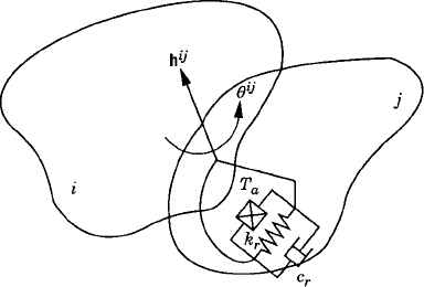
We now consider the case of a rotational spring-damper-actuator element (Fig. 10) that connects two arbitrary bodies i and j in the multibody system. These two bodies may be connected by a revolute, screw, or cylindrical joint. Let θij be the rotation of body i with respect to body j along the joint axis, and let hij be a unit vector along the joint axis. The virtual change δθij can be expressed in terms of the generalized orientation coordinates of bodies i and j as
This equation implies that the virtual relative rotation δθij is the projection of the relative Cartesian rotation
The torque exerted on body i by the rotational spring-damper-actuator element as the result of the rotation θij is
where kr and cr are, respectively, the rotational spring and damping coefficients, and Ta is the actuator torque. The coefficients kr and cr and the torque Ta can be nonlinear functions of the system coordinates, velocities, and time.
The virtual work of the torque Tij is
This equation can also be written as
where the generalized forces Qi and Qj are given by
In the preceding two sections, the virtual work of the inertia forces and the virtual work of the applied forces acting on the rigid body i were developed. It was shown that the virtual work of the inertia forces can be written as (Eq. 95)
where Mi is the symmetric mass matrix,
The virtual work of the applied forces is
where Qie is the vector of generalized applied forces.
Using the principle of virtual work in dynamics for unconstrained motion, one has
Substituting Eqs. 172 and 173 into Eq. 174, one obtains
or
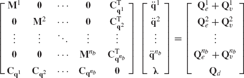
In the case of unconstrained motion, the elements of the vector δqi are independent. In this case, Eq. 176 leads to
where nb is the total number of rigid bodies in the system. The preceding equation can be written in a partitioned matrix form as
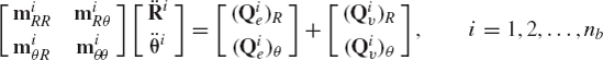
where miRR,
Equation 178 is the matrix equation that governs the unconstrained motion of the rigid body. This equation can be simplified if the origin of the body coordinate system is rigidly attached to the center of mass of the body. In this case
It follows also that
Substituting this equation into Eq. 100, one obtains
which imply that in the case of a centroidal body coordinate system, there is no inertia coupling between the translation and the rotation of the rigid body. Furthermore, in this special case
The use of Eqs. 181, 182, and 178 leads to the following dynamic equations:
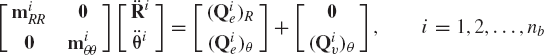
where, as previously defined by Eqs. 100 and 134,

When Euler angles are used, the set of orientation coordinates θi has three elements and the mass matrix in Eq. 183 is a 6 × 6 matrix.
Example 7.8
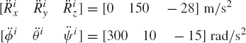
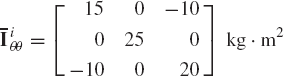
A force vector Fi = [5.0 0.0 −3.0]T N is acting on unconstrained body i. The orientation of a centroidal body coordinate system is defined by the Euler angles
The time rate of change of Euler angles at the given configuration is
The local position vector of the point of application of the force is
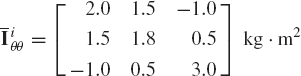
The mass of the body is 2 kg and its inertia tensor is
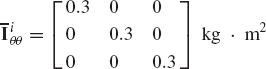
Write the equations of motion of this system at the given configuration and determine the accelerations.
Solution. The transformation matrix that defines the orientation of the body is
At the given configuration, one also has
It was shown in Example 7 that the generalized forces associated with the translation and the orientation coordinates of the body reference are
Using the mass of the body, one has
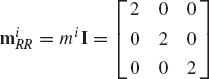
and
Since a centroidal body coordinate system is used
The angular velocity vector in the body coordinate system is
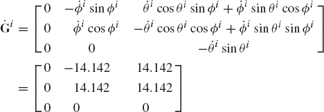
Using Euler angles and their time derivatives, one has
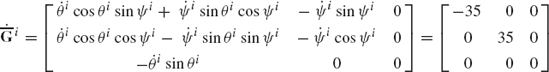
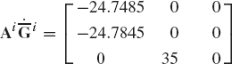
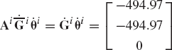
It follows that
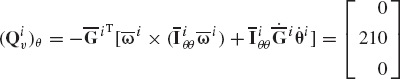
The quadratic velocity inertia force vector associated with the translation of the body reference is equal to zero since a centroidal body coordinate system is used, while the force vector associated with the orientation coordinates is
Using the case of the centroidal body coordinate system, the matrix equation of motion of the body can be written as
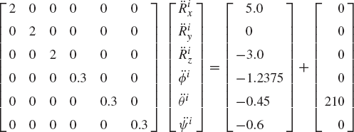
or
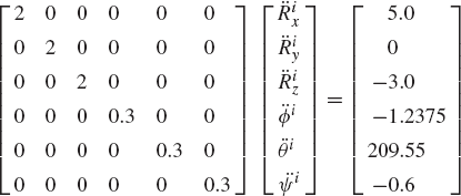
The solution of this system of equations defines the accelerations as
The results obtained in this example can also be used to show that
while
Nonetheless,
remains in effect.
As in the case of planar analysis, there are different approaches for formulating the dynamic equations of constrained spatial multibody systems. The first approach, in which a set of independent coordinates are used in the formulation of the dynamic relationships, leads to the smallest set of differential equations expressed in terms of the system degrees of freedom. This method will be discussed in more detail in Section 14 of this chapter. An alternative approach that is discussed in this section is to use the augmented formulation, wherein the dynamic equations are formulated in terms of a set of dependent and independent coordinates. The kinematic relationships that describe mechanical joints and specified motion trajectories are adjoined to the system differential equations using the technique of Lagrange multipliers. This approach leads to a relatively large system of loosely coupled equations that can be solved using matrix, numerical, and computer methods.
Consider a multibody system that consists of nb interconnected bodies. In the analysis presented in this section, the configuration of each body in the multibody system is described using the absolute Cartesian coordinates Ri and the orientation coordinates θi. The vector of system-generalized coordinates can be written as
which can also be written as
where
The kinematic relationships that describe mechanical joints and specified motion trajectories such as driving constraints can be written in the following vector form:
If the number of kinematic constraint equations is equal to the number of the generalized coordinates, the system is said to be kinematically driven, and in this case, Eq. 188 can be solved for the generalized coordinates using a Newton-Raphson algorithm.
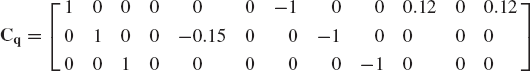
The velocity kinematic equations can be obtained by differentiating Eq. 188 with respect to time, yielding
where Cq is the constraint Jacobian matrix and Ct is the vector of partial derivatives of the constraint equations with respect to time. The Jacobian matrix is obtained by differentiating the constraint equations with respect to the coordinates, while the vector Ct is defined as
The vector Ct is the zero vector if the constraint equations are not explicit functions of time. If the constraint equations are linearly independent, the constraint Jacobian matrix has a full row rank, and in the case of kinematically driven systems, the Jacobian matrix becomes a square matrix. In this special case, Eq. 189 can be considered as a linear system of algebraic equations in the velocities, and this system has a unique solution that can be determined assuming that the generalized coordinates are known from solving Eq. 188.
The kinematic acceleration equations can be obtained by differentiating Eq. 189 with respect to time. This leads to
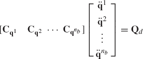
where Qd is a vector that absorbs terms that are quadratic in the velocities. This vector is defined as
Equation 191 can be considered as a linear system of algebraic equations in the accelerations, and in the case of kinematically driven systems, Eq. 191 has a unique solution that determines the vector of generalized accelerations.
It is clear that the kinematic equations of the spatial multibody systems are similar to the equations obtained in the case of planar systems. Consequently, the numerical algorithms used in the spatial kinematic analysis have the same steps as the algorithms used in the planar kinematic analysis. These algorithms were discussed in detail in Chapter 3.
In the formulation of the dynamic equations using the absolute coordinates, the technique of Lagrange multipliers is used to adjoin the kinematic constraint equations to the differential equations of motion. For body i in the system, the equations of motion can be written in a matrix form as
where Mi is the body mass matrix,
Equations 193 and 194 can be combined in order to obtain the following matrix equation:
which can also be written as
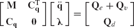
This equation can be solved for the vectors of accelerations and Lagrange multipliers. The vector of Lagrange multipliers can be used to determine the generalized constraint forces
In the analysis presented in this book, the kinematic constraints are classified as joint or driving constraints. Joint constraints define the connectivity between bodies in the system, while driving constraints describe the specified motion trajectories. The driving constraints may depend on time and may take any form depending on the particular application. On the other hand, in the case of using the absolute coordinates in the analysis of mechanical systems, the formulation of the kinematic constraints that describe a joint between two arbitrary bodies in the system can be made independent of the particular topological structure of that system since similar sets of coordinates are used to describe the motion of the bodies. A computer library that contains the formulations of a number of mechanical joints that are often encountered in the analysis of mechanical systems can be developed and used in the computer-aided analysis of a variety of applications. In this section, the formulations of some of the mechanical joints used in spatial multibody systems are discussed.
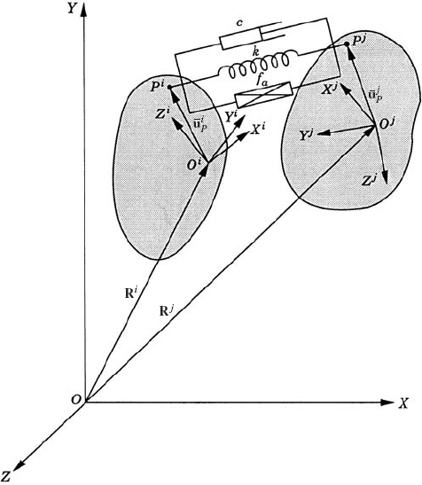
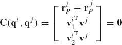
Figure 11 shows two bodies, i and j, connected by a spherical joint which eliminates the freedom of relative translations between the two bodies, and it allows only three degrees of freedom of relative rotations. The kinematic constraints of the spherical joint require that two points, Pi and Pj on bodies i and j, respectively, coincide throughout the motion. This condition can be written as
where Ri and Rj are the global position vectors of the origins of the coordinate systems of bodies i and j, respectively; Ai and Aj are the transformation matrices of the two bodies; and
where
Therefore, a virtual change in the kinematic constraints of the spherical joint leads to
This equation can be expressed in matrix form as
which can be written as
where Cq is the Jacobian matrix of the spherical joint constraints defined as
This Jacobian matrix can also be written as
where
Example 7.9
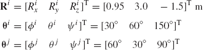
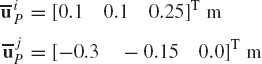
Two bodies i and j are connected by a spherical joint. The orientation of the two bodies are defined by the Euler angles
The local position vectors of the joint definition point on bodies i and j are defined, respectively, by the vectors
Using the absolute Cartesian coordinates and Euler angles as the generalized coordinates, obtain the Jacobian matrix of the kinematic constraints of this two-body system at the given configuration.
Solution. The transformation matrices that define the orientation of the two bodies are
Using Eq. 81, it can be shown, at the given configuration, that
The Jacobian matrix of the kinematic constraints is
where
Thus,
where each row corresponds to one of the constraint equations of the spherical joint and each column corresponds to one of the generalized coordinates ordered as defined in the vector q.
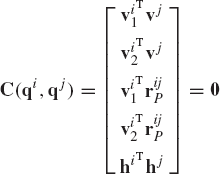
Figure 12 shows a cylindrical joint that allows relative translation and rotation between body i and body j along the joint axis. The joint has two degrees of freedom because it eliminates the freedom of four possible independent relative displacements between the two bodies. The cylindrical joint constraints can, therefore, be described using four algebraic equations. Let vi and vj be two vectors defined along the joint axis on body i and body j, respectively, and let Pi and Pj be two points on body i and body j, defined along the joint axis. The constraint equations for the cylindrical joint can be defined as
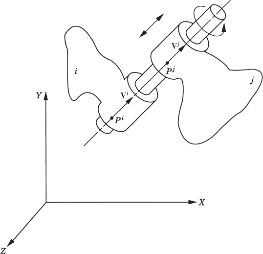
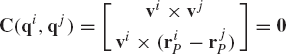
Since each of the cross products in the preceding equation defines two independent equations only, the preceding equation defines four independent kinematic relationships.
An alternative for the use of the cross product is to use two independent dot product equations as described in Chapter 2. In this case, two vectors vi1 and vi2 are defined on body i such that vi, vi1, and vi2 form an orthogonal triad. The constraint equations for the cylindrical joint can then be defined as
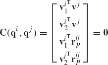
where rijP is defined as
A simple computer procedure for defining the vectors vi1 and vi2 was described in Chapter 2.
The Jacobian matrix of the cylindrical joint constraint equations can be written as
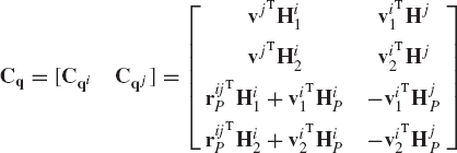
where HiP and Hjp are as defined by Eq. 205, and
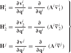
in which
The revolute joint has one degree of freedom and can be considered as a special case of the cylindrical joint by eliminating the freedom of the relative translation between the two bodies. In order to preclude the relative translation between the two bodies, the distance between point Pi on body i and point Pj on body j (Fig. 12), both defined along the joint axis, must remain constant, that is,
where kr is a constant and
Equation 211 is a scalar equation that when added to the constraints of the cylindrical joint, as defined by Eq. 207, leads to
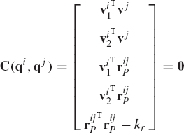
This system of equations has five independent constraint equations.
The Jacobian matrix of the revolute joint constraints is
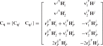
where all the variables that appear in this equation are the same as the ones used in the case of the cylindrical joint.
Another alternate approach for formulating the revolute joint constraints is to consider it as a special case of the spherical joint in which the relative rotation between the two bodies is allowed only along the joint axis. If point P is the joint definition point as defined in the case of the spherical joint, and vi and vj are two vectors defined along the joint axis on bodies i and j, respectively, the constraint equations of the revolute joint can be written as
The last two equations in Eq. 215 guarantee that the two vectors vi and vj remain parallel, thereby eliminating the freedom of the relative rotation between the two bodies in two perpendicular directions.
The Jacobian matrix of the revolute joint constraints as defined by Eq. 215 is

where the matrices HiP, Hjp, Hi1, and Hi2 are as defined by Eqs. 205 and 210, respectively.
The single-degree-of-freedom prismatic joint can also be obtained as a special case of the cylindrical joint by eliminating the freedom of the relative rotation between the two bodies about the joint axis. The two orthogonal vectors hi and hj drawn perpendicular to the joint axis are defined on bodies i and j, respectively, as shown in Fig. 13. In order to preclude the relative rotation between the two bodies, one must have
This equation can be added to the constraint equations of the cylindrical joint, as defined by Eq. 207, in order to define the constraint equations of the prismatic joint as
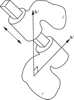
This vector equation has five independent constraint equations that depend only on the generalized coordinates of bodies i and j.
The Jacobian matrix of the prismatic joint constraints is
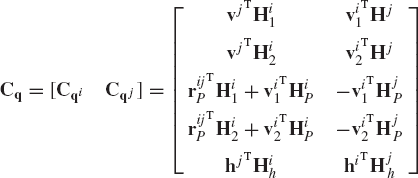
where
in which
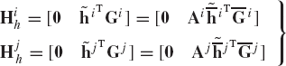
The universal joint shown in Fig. 14 is a two-degree-of-freedom joint. Let point P be the point of intersection of the two bars of the joint cross, as shown in the figure. The coordinates of this point in the coordinate systems of bodies i and j are constant. Let hi and hj be two orthogonal vectors defined along the intersecting axes of the joint on bodies i and j, respectively. The constraint equations of the universal joint can be written as
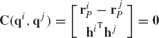
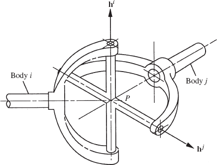
where riP and rjp are the global position vectors of point P defined using the generalized coordinates of bodies i and j, respectively.
The Jacobian matrix of the universal joint constraints is
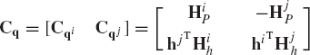
where the matrices HiP, Hjp, Hih, and Hjh are as previously defined.
A rigid joint between two rigid bodies i and j does not allow any freedom of relative translation or relative rotation between the two bodies. The rigid joint is described using six constraint equations that can be written as
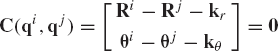
where kr and kθ are two constant vectors.
The Jacobian matrix of the rigid joint can simply be written as
A special case of the rigid joint concerns the ground constraints. If, for example, body i is the fixed link (ground), one has
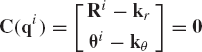
where kr and kθ are constant vectors. The preceding constraint equations eliminate the freedom of body i to translate or rotate.
It is clear from the discussion presented in this section that most of the joint kinematic constraint equations can be formulated in terms of simple vector addition and/or scalar product. For instance, the following basic vector operations were used in formulating the joint constraints between body i and body j:
where c is a constant vector, vi and vj are vectors defined on body i and body j, respectively, and rijP is as defined by Eq. 212. The preceding three basic equations and their partial derivatives with respect to the generalized coordinates can be used to develop a computer library that can be used in formulating many of the joint constraint equations described in this section.
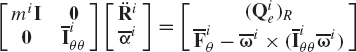
In the Newton-Euler formulation, the equations of motion of the rigid body are expressed in terms of the angular velocity and acceleration vectors. It is also assumed that the origin of the body coordinate system (reference point) is the center of mass of the body. Using this assumption and the relationships between the angular velocity and acceleration vectors, and the orientation coordinates, it can be shown that Eq. 183 leads to
where αi and ωi are, respectively, the angular acceleration and velocity vectors defined in the global coordinate system, mi is the mass of the rigid body,
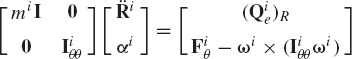
or
where
As pointed out previously, the angular velocities in the spatial analysis are not, in general, the time derivatives of a set of orientation coordinates. For this reason, the angular accelerations obtained by solving Newton-Euler equations cannot be integrated directly in order to obtain the system coordinates. One must first determine the second derivatives of the generalized orientation coordinates as a function of the angular accelerations. The second derivatives of the generalized orientation coordinates can then be integrated to determine the generalized coordinates and velocities. In the recursive methods discussed in Section 14, however, the angular velocity and acceleration vectors are expressed in terms of the joint coordinates and their first and second time derivatives. The joint accelerations can be determined and can be integrated numerically in order to determine the joint angles and joint velocities.
The coefficient matrix in the Newton-Euler equations of Eq. 229 can be made constant if the angular acceleration is defined in the body coordinate system. Recall that
In this equation,
In this form of the Newton-Euler equations, the coefficient matrix is constant since the inertia tensor is defined in the body coordinate system.
In this chapter, the virtual work principle was used to obtain the Newton-Euler equations. As in the case of the planar analysis discussed in Chapter 4, the Newton-Euler equations can be derived in a straightforward manner by applying D'Alembert's principle. The procedure for doing that is outlined in this section.
If the rigid body i is assumed to consist of a large number of particles, each of which has mass ρidVi where ρi is the mass density and dVi the infinitesimal volume, the inertia force of a particle whose position vector ri is equal to
In this equation, (Qie)R is the vector of resultant forces acting on the body. The preceding equation, as in the case of the planar analysis, allows using any point as the reference point. Recall that the absolute acceleration of an arbitrary point on the rigid body can be written as
where Ri is the global position vector of the reference point on the body; ωi and αi are, respectively, the angular velocity and angular acceleration vectors of the body;
Substituting Eq. 235 into Eq. 234 and using the identity of Eq. 236 and the fact that ωi and αi do not depend on the location of the arbitrary point, one obtains
or
which is the Newton equation of motion.
Euler equation can be obtained from D'Alembert's principle by treating the inertia forces as the applied forces. To this end, it is assumed again that the rigid body i consists of a large number of particles. The moment of the inertia force of a particle about an arbitrary reference point is
In this equation, Fiθ is as defined in the preceding section.
In order to obtain Euler equation, the reference point is chosen to be the body center of mass. Substituting Eq. 235 into Eq. 239, and using the identity of Eq. 236, one can show that
This equation can be written as
which is the Euler equation obtained in the preceding section.
Newton-Euler equations can also be derived using the principle of linear and angular momentum. The linear momentum of a rigid body is defined as
where
where Ri, in this case, is the global position vector of the center of mass of the rigid body.
Newton's law of motion states that the rate of change of the linear momentum is equal to the vector of the resultant force acting on the body, that is
which leads to Newton's equations
The angular momentum of the rigid body i is defined as
which upon the use of Eqs. 84 and 180 and the definition of the linear momentum reduces to
where
where
where the fact that
The rate of change of the angular momentum
which leads to Euler equations
This equation can also be expressed in terms of vectors defined in the centroidal body coordinate system as
which upon premultiplying by AiT yields
where
It is clear from the preceding discussion that if there are no forces or moments acting on the rigid body, one gets
which imply that the linear and angular momentum are constants of motion.
Example 7.10
Consider the rigid body whose inertia tensor defined in a centroidal body coordinate system is
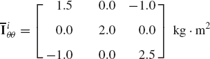
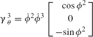
The body rotates with a constant angular velocity such that
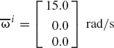
Determine the components of the external moments applied to this body.
Solution. Euler's equation defined in the body coordinate system is
Since the angular velocity vector is constant, it follows that
Euler's equation reduces in this case to
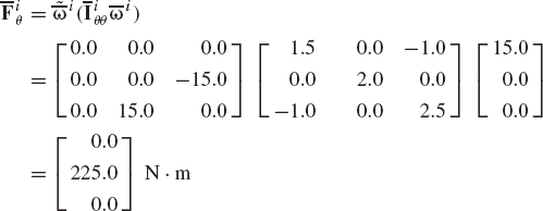
It can be seen from these results that the applied moment is constant in the body coordinate system. This moment is equal in magnitude and opposite in direction to the inertial moment due to the centrifugal force.
As pointed out previously, one of the major advantages of using the absolute coordinates is that the motion of each body in the multibody system is described using similar sets of generalized coordinates that do not depend on the topological structure of the system. The mass matrices of the bodies in the system have similar form and dimensions, such that a computer program with simple structure can be developed based on the augmented formulation. A library of standard joint constraints can also be developed and used as a module in this computer program. One disadvantage, however, of using the augmented formulation is the complexity of the numerical algorithm that must be used to solve the resulting mixed system of differential and algebraic equations.
Other alternate approaches for formulating the equations of motion of constrained mechanical systems are the recursive methods, wherein the equations of motion are formulated in terms of the joint degrees of freedom. This formulation leads to a minimum set of differential equations from which the workless constraint forces are automatically eliminated. The numerical procedure used in solving these differential equations is much simpler than the procedure used in the solution of the mixed system of differential and algebraic equations resulting from the use of the augmented formulation.
There are several techniques for formulating the recursive dynamic equations of multibody systems. These techniques eventually lead to the same equations if the same set of joint variables is used. In fact, the equivalence of these techniques can be demonstrated using simple coordinate transformations. One of the approaches used for formulating the dynamic recursive equations is based on Newton-Euler equations that are expressed in terms of the angular accelerations. We discuss this approach in this section in order to have a better understanding of the basic joint-force relationships in the analysis of interconnected bodies. By so doing, we will have an appreciation of the principle of virtual work in dynamics, which can also be used to obtain the same recursive dynamic equations presented in this section.
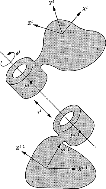
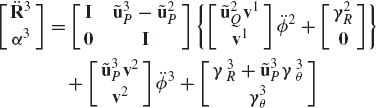
In order to illustrate the development of the recursive kinematic equations, we consider the two bodies i−1 and i, which are connected by a cylindrical joint as shown in Fig. 15. The two-degree-of-freedom cylindrical joint allows relative translation along, and relative rotation about the joint axis. If τi and ϕi denote, respectively, the relative translation and rotation between the two bodies, the following kinematic relationships between the absolute and relative coordinates hold:
where
and the vector vi−1 can be written as
where
Similarly, differentiating Eq. 257 with respect to time, one obtains
Differentiating the first equation in Eq. 256 twice with respect to time and the second equation once with respect to time and using Eqs. 259 and 260, one obtains

and
Using the skew-symmetric matrix notation, the preceding two equations can be written as
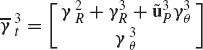
where γiR and γiθ are vectors that absorb terms that are quadratic in the velocities. Those vectors are defined as
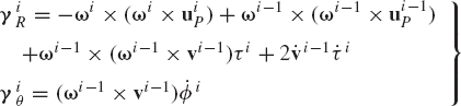
Equations 263 and 264 can be combined into one matrix equation as
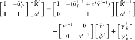
Note that
Using this equation, Eq. 266 leads to

which can also be written as
where
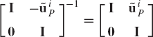
The matrix Di can be written as
and
The matrix Di satisfies the following identities:
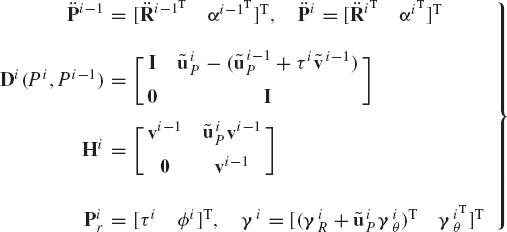
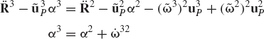
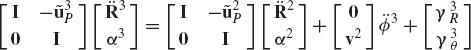
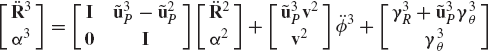
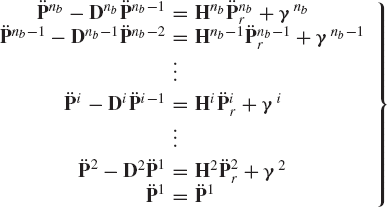
In Eq. 269, the vector of accelerations of body i is expressed in terms of the accelerations of body i − 1 and the vector of joint accelerations
Since Eq. 269 is developed for two arbitrary bodies, one also has
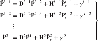
where body 1 is considered as the base body.
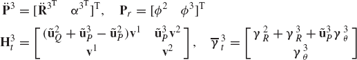
Substituting Eq. 274 into Eq. 269, the accelerations of body i can be expressed in terms of the accelerations of the base body and the joint accelerations as
where Pr is the vector of the system joint degrees of freedom, Dit and Hit are velocity influence coefficient matrices, and γit is a vector that absorbs terms that are quadratic in the velocities. The vector Pr is given by
where Pkr is the vector of the degrees of freedom of the joint connecting bodies k and k − 1, and
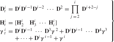
in which
If the motion of the base body is specified, Eq. 275 can be written as
where
Example 7.11
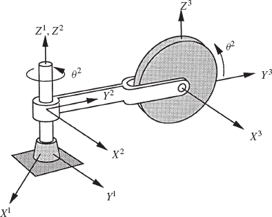
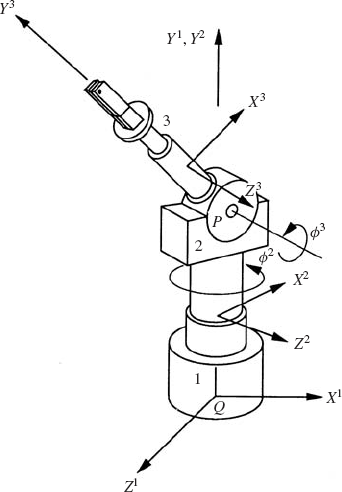
Figure 16 shows a two-degree-of-freedom robotic manipulator which consists of three bodies including the ground (body 1). Body 2 is connected to body 1 by a revolute joint at point Q, and the axis of this joint is along the Y1 axis. Body 3 is connected to body 2 by a revolute joint at point P, and the axis of this revolute joint is assumed to be parallel to the Z2 axis. Obtain the recursive kinematic relationships of this system.
Solution. Since body 2 is rotating about the Y1 axis, the transformation matrix that defines the orientation of this body is given by
where ϕ2 is the degree of freedom of the joint at point Q. Similarly, since body 3 rotates about an axis parallel to the Z2 axis, the orientation of this body with respect to body 2 is defined by the matrix
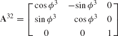
where ϕ3 is the degree of freedom of the second revolute joint.
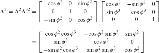
The transformation matrix that defines the orientation of body 3 with respect to body 1 is then given by
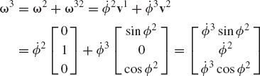
Equation 256 can be used to describe the connectivity between bodies 2 and 3 as
where
in which
This defines ω32 as
which upon differentiation yields
where
By differentiating the kinematic relationships of the revolute joint at P, one obtains
or
where
and
It follows that
This equation can also be obtained as a special case of Eq. 268 or equivalently, Eq. 269, that describes the more general two-parameter screw motion. It is clear from the preceding equation that the matrix H3 reduces in the case of revolute joint to a six-dimensional vector since the revolute joint has only one degree of freedom.
For the revolute joint between body 2 and body 1, similar kinematic relationships can be obtained. Nonetheless, the resulting equations can be simplified since body 1 is fixed in space. In this case, one has
where u~2Q is the skew-symmetric matrix associated with the vector
and
The absolute acceleration of body 3 can then be expressed in terms of the joint variables as
which can be written in the form of Eq. 279 as
where
We note also from the preceding equations that the angular velocity of body 3 can be expressed in terms of the joint rates as
Using the results obtained in this example, one can also verify that
and
Equation 279, in which the accelerations of body i are expressed in terms of the joint accelerations, can be used with Newton-Euler equations to obtain a minimum set of differential equations expressed in terms of the joint degrees of freedom. If Eq. 279 is substituted into Newton-Euler equations of body i as defined by Eq. 230, one gets
where Fic is the vector of joint reaction forces acting on body i. Premultiplying Eq. 281 by
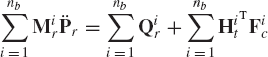
which can be written as
where nb is the total number of bodies, and
Note that Mir is a square matrix whose dimension is the same as the number of the system joint degrees of freedom. Since Eq. 283 is developed for an arbitrary body in the system, one has
Utilizing the fact that
one obtains
where Mr is the generalized system mass matrix associated with the joint degrees of freedom, and Qr is the vector of generalized forces. The matrix Mr and the vector Qr are given by
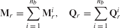
Since the kinetic energy is a positive definite quadratic form, the system mass matrix Mr is nonsingular, and Eq. 287 can be solved for the joint accelerations as
These accelerations can be integrated numerically forward in time using a direct numerical integration method. The numerical solution defines the joint coordinates and velocities. Once the joint variables are determined, the absolute variables can be determined by using the kinematic relationships.
Example 7.12
Use the recursive kinematic relationships obtained in Example 11 to derive the independent differential equations of motion of the two degree of freedom robotic manipulator shown in Fig. 16.
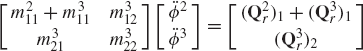
Solution. Newton-Euler equations of body 3 can be written in the following matrix form:
or
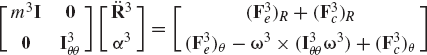
This equation can be expressed in terms of the joint degrees of freedom using the kinematic equations obtained in Example 11. It was shown that the acceleration kinematic relationships are
where
and
Using Eq. 283, one has
where
in which
The vector Q3r is given by
where
Similarly, for body 2, one has
where, as shown in Example 11,
It follows that
where
where
The system equations of motion can then be written in terms of the joint degrees of freedom using Eq. 287 as
The recursive method presented in this section can also be extended to the analysis of open-chain multibody systems with multiple branches. The use of this approach in the dynamic analysis of such systems has two major computational advantages over the augmented formulations that employ Lagrange multipliers. The first advantage is that a minimum set of differential equations is obtained. As a result of that, the constraint forces are automatically eliminated since the dynamic equations are expressed in terms of the joint degrees of freedom. The second advantage is the simplicity of the numerical scheme used for the solution of the dynamic equations developed using the recursive methods. There is no need for using a Newton-Raphson algorithm since the recursive formulation of the equations of open kinematic chains leads only to a set of differential equations. One disadvantage of using the recursive method, however, is that the dynamic equations are expressed in terms of a set of joint variables that depend on the topological structure of the multibody system. For that reason, it is more difficult to develop general-purpose multibody computer programs based on the recursive methods. These methods also become less attractive in the analysis of closed-chain mechanical systems. One approach for dealing with closed-chain systems using the recursive methods is to make cuts at selected secondary joints to form spanning tree structures. The method of analysis presented in this section can then be used to develop the equations of motion of the resulting open-chain branches. Connectivity conditions between the branches at the secondary joints can be handled by either eliminating the dependent variables or by using the method of Lagrange multipliers. In the case of Lagrange multipliers, the recursive formulation leads to a mixed system of differential and algebraic equations that must be solved using the same numerical procedure used in the case of the augmented formulation.
Another elegant approach similar, in principle, to the methods discussed in Chapter 6 can be used for deriving the recursive kinematic and dynamic equations of spatial mechanical systems. In this approach, Eq. 274 can be written for nb bodies as
which leads to
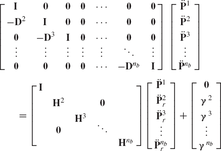
This equation can be written as
where
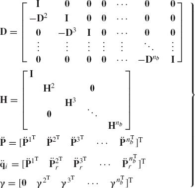
The matrix D can be written as the product of nb−1 matrices as follows:
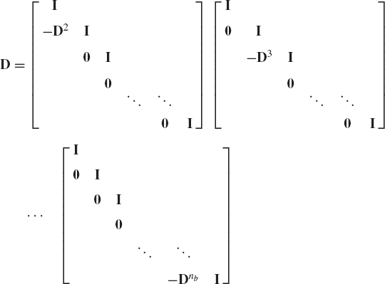
from which
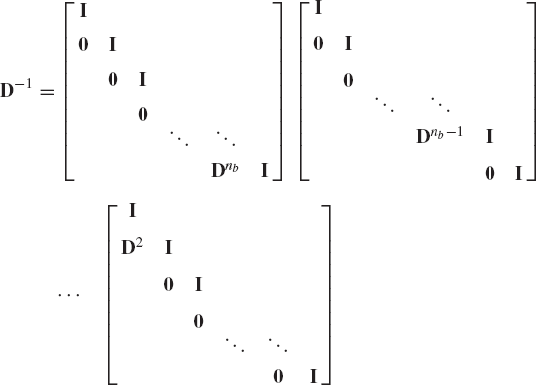
or
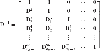
where
The absolute accelerations can then be expressed in terms of the joint accelerations as
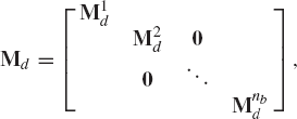
where Bi = D−1H and
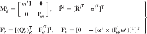
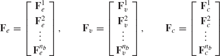
where Md is the block diagonal mass matrix, Fe is the vector of applied forces, Fv is the vector of centrifugal forces, and Fc is the vector of constraint forces. The matrix Md is defined as
and the vectors Fe, Fv, and Fc are defined as
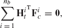
Substituting the kinematic acceleration equations into the dynamic equations of motion and premultiplying by BTi, one obtains
Since these equations are expressed in terms of the independent joint accelerations one must have
Using the preceding two equations, the independent differential equations of motion of the system reduce to
where
If the axes Xi, Yi, and Zi of the coordinate system of body i are defined in the coordinate system XYZ by the vectors [0.5 0.0 0.5]T, [0.25 0.25 −0.25]T, and [−2.0 4.0 2.0]T, respectively, use the method of direction cosines to determine the transformation matrix that defines the orientation of body i in the coordinate system XYZ.
The axes Xi, Yi, and Zi of the coordinate system of body i are defined in the coordinate system XYZ by the vectors [0.0 1.0 1.0]T, [−1.0 1.0 −1.0]T, and [−2.0 −1.0 1.0]T, respectively. Use the method of the direction cosines to determine the transformation matrix that defines the orientation of the rigid body i in the coordinate system XYZ.
The axes Xi, Yi, and Zi of the coordinate system of the rigid body i are defined in the coordinate system XYZ by the vectors [0.0 −1.0 1.0]T, [−1.0 1.0 1.0]T, and [−2.0 −1.0 −1.0]T, respectively. Determine the transformation matrix of body i using the method of the direction cosines.
The axes Xi, Yi, and Zi of the coordinate system of the rigid body i are defined in the coordinate system XYZ by the vectors [0.0 1.0 1.0]T, [−1.0 1.0 −1.0]T, and [−2.0 −1.0 1.0]T, respectively. The axes Xj, Yj, and Zj of the coordinate system of body j are defined in the coordinate system XYZ by the vectors [0.0 −1.0 1.0]T, [−1.0 1.0 1.0]T, and [−2.0 −1.0 −1.0]T, respectively. Use the method of the direction cosines to define the orientation of body i with respect to body j. Define also the orientation of body j with respect to body i.
The axes of the coordinate system of body i are defined in the XYZ coordinate system by the vectors [1.0 0.0 1.0]T, [1.0 1.0 −1.0]T, and [−1.0 2.0 1.0]T. Use the method of the direction cosines to define the orientation of body i in the coordinate system of body j whose axes are defined by the vectors [0.0 −1.0 1.0]T, [−1.0 1.0 1.0]T, and [−2.0 −1.0 −1.0]T.
In problem 1, if body i rotates an angle θi1 = 45° about its Zi axis followed by another rotation θi2 = 60° about its Xi axis, determine the transformation matrix that defines the orientation of the body in the XYZ coordinate system as the result of these two consecutive rotations.
In problem 2, if body i rotates an angle θi1 = 90° about its Yi axis followed by a rotation θi2 = 30° about its Xi axis, determine the transformation matrix that defines the orientation of the rigid body as the result of these two consecutive rotations.
If the rigid body i in problem 3 rotates an angle θi1 = 60° about its Xi axis, and an angle θi2 = 45° about its Zi axis, determine the transformation matrix that defines the final orientation of the body in the XYZ coordinate system.
Obtain the transformation matrix in terms of Euler angles if the sequence of rotations is defined as follows: a rotation ϕi about Zi axis, a rotation θi about Yi axis, and a rotation ψi about Xi axis.
Obtain the transformation matrix in terms of Euler angles if the sequence of rotation is defined as follows: a rotation ϕi about Zi axis, a rotation θi about Yi axis, and a rotation ψi about Zi axis.
Use the transformation obtained in problem 1 to extract the three Euler angles by considering the sequence of rotation described in Section 3. If the origin of the body coordinate system is defined by the vector Ri = [−1.5 0.4 3.2]T, determine the global position vector of point Pj whose local coordinates are defined by the vector
Use the transformation matrix obtained by solving problem 2 to extract the three Euler angles using the sequence of rotation described in Section 3. If the origin of the body coordinate system is defined by the vector Ri = [2.1 3.4 −11.0]T, determine the global position vector of point Pi whose position vector in the body coordinate system is defined by the vector
Use the general development presented in Section 4 to define the angular velocity vector ωi in the following two cases: (a) a simple rotation about the global X axis, and (b) a simple rotation about the global Y axis.
Use the general development presented in Section 4 to define the angular velocity vector ωi in the following two cases: (a) a simple rotation about the global X axis, and (b) a simple rotation about the global Y axis.
The angular velocity in the body coordinate system is defined by Eq. 83 as

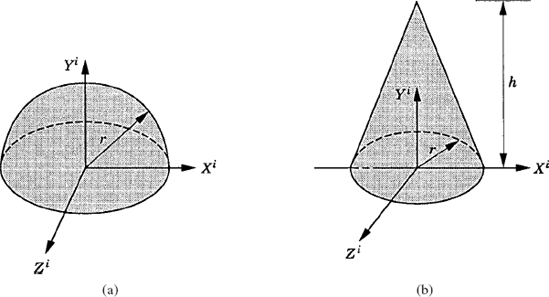
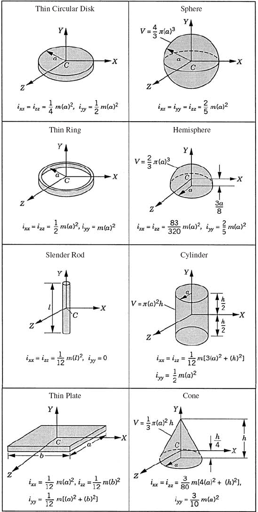
Use Eq. 118 to determine the location of the center of mass of the hemisphere and right circular cone shown in Fig. P1.
Determine the elements of the inertia tensor of a right circular cylinder with radius r and length h with respect to a centroidal coordinate system.
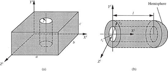
Determine the elements of the inertia tensor of hollow cylinder with inner and outer radii ri and ro, respectively, and length h. Use a centroidal coordinate system.
Using a centroidal coordinate system, determine the elements of the inertia tensor of the hemisphere and right circular cone shown in Fig. P1. Use the parallel axes theorem to determine the moments of inertia in the coordinate system XiYiZi shown in the figure.
Determine the elements of the inertia tensor of the composite bodies shown in Fig. P2 in the coordinate systems shown in the figure.
In problem 11, let the rigid body be subjected to a moment whose components are defined in the global coordinate system by
Obtain the generalized forces associated with Euler angles as the result of the application of the moment Mia.
In problem 11, let the rigid body be subjected to the forces
and the moment
The coordinates of the point of application of the forces Fi1 and Fi2 are given, respectively, by
Assuming that the forces and the moment are defined in the global coordinate system, obtain the generalized forces associated with the translation and orientation coordinates of the rigid body. Use Euler angles as the orientation coordinates.
Repeat the preceding problem assuming that the forces and the moment are defined in the body coordinate system.
A force vector Fi = [3.0 0.0 −8.0]T N is acting on unconstrained body i. The orientation of a centroidal body coordinate system is defined by the Euler angles
The time rate of change of Euler angles at the given configuration is
The local position vector of the point of the application of the force is
The mass of the body is 5 kg and its inertia tensor is
Write the equations of motion of this system at the given configuration and determine the accelerations.
A force vector Fi = [9.0 7.0 −12.0]T N is acting on unconstrained body i. The orientation of a centroidal body coordinate system is defined by the Euler angles
The time rate of change of Euler angles at the given configuration is
The local position vector of the point of the application of the force is
The mass of the body is 3 kg and its inertia tensor is
Write the equations of motion of this system at the given configuration and determine the accelerations.
The orientation of a centroidal body coordinate system of unconstrained body i is defined by the Euler angles
The time rate of change of Euler angles at the given configuration is
and the second time derivatives of the coordinates are
The mass of the body is 4 kg and its inertia tensor is
Determine the resultant external force vector acting at the center of mass as well as the external moment vector acting on the body.
Determine the vector Qd of Eq. 191 in the case of the spherical joint.
Determine the vector Qd of Eq. 191 in the case of the cylindrical joint.
Determine the vector Qd of Eq. 191 in the case of the revolute joint.
Two bodies i and j are connected by a spherical joint. Let
The position vectors of the joint definition points on body i and body j defined in the respective body coordinate systems are given by
Determine the vector Rj and the Jacobian matrix of the spherical joint constraints.
Using Eq. 183 as the starting point, derive Newton-Euler equations.
The inertia tensor of a rigid body defined in a centroidal body coordinate system is given by
The body rotates with a constant angular velocity equal to 20 rad/s about its Yi axis. Determine using Newton-Euler equations the external moments applied to this body.
Determine the velocity influence coefficient matrices Di and Hi and the vector γi of Eq. 269 in the case of the revolute joint.
Determine the velocity influence coefficient matrices Di and Hi and the vector γi of Eq. 269 in the case of prismatic joint.
Determine the velocity influence coefficient matrices Di and Hi and the vector γi of Eq. 269 in the case of spherical joint.
Use the principle of virtual work in dynamics to obtain the recursive formulation of Eq. 287.
Figure P3 shows a disk, denoted as body 3, which rotates about its X3 axis with an angle θ3. The supporting arm, denoted as body 2, rotates with an angle θ2 about its Z2 axis. Determine the absolute angular velocity vector of the disk in the fixed X1Y1Z1 coordinate system. Determine also the components of this angular velocity vector in the disk coordinate system.
Obtain the recursive kinematic relationships of the system of Example 11, if body 1 rotates about its X1 axis with an angle ϕ1. Assume that the X1 axis is fixed in space. Determine the absolute angular velocity and acceleration vectors of bodies 2 and 3 in terms of the joint variables ϕ1, ϕ2, and ϕ3 and their time derivatives.
In the preceding problem, determine the recursive dynamic equations using the Newton-Euler formulation. Obtain the system of independent differential equations and identify the mass matrix associated with the joint degrees of freedom.