
6
Light
6.1 Introduction
Light is a form of radiation and physical laws have been constructed to explain its behaviour. The general science of radiation is called radiometry. However, physical laws cannot explain the sense we call vision or the impression of colour. For applications of imaging technology such as television and cinema, light is what can be seen by a human being and this is the subject of photometry. In that context, any discussion must include the characteristics of the eye in all the relevant domains. Once the operation of the human visual system (HVS) is understood, it will be clear that, in order to obtain realism, imaging quality has to meet adequate criteria in a number of domains. These include at least contrast, noise level, colour accuracy, static and dynamic resolution, flicker and motion portrayal.
Once these topics are appreciated, it then becomes possible to analyse today’s popular imaging technologies to see why they all look different and to suggest a way forward to a new level of realism which will be expected in applications such as simulators and electronic cinema.
Figure 6.1 shows some of the interactions between domains which complicate matters. Technically, contrast exists only in the brightness domain and is independent of resolution which exists in the image plane. In the HVS, the subjective parameter of sharpness is affected by both and so these cannot be treated separately. Sharpness is also affected by the accuracy of motion portrayal. It would appear that colour vision evolved later as an enhancement to monochrome vision. The resolution of the eye to colour changes is very poor.

6.2 What is light?
Electromagnetic radiation exists over a fantastic range of frequencies, f, and corresponding wavelengths λ connected to the speed of light, c, by the equation:
c = f × λ
The human visual system (HVS) has evolved to be sensitive to a certain range of frequencies which we call light. The frequencies are extremely high and it is the convention in optics to describe the wavelength instead. Figure 6.2 shows that the HVS responds to radiation in the range of 400 to 700 nanometres (nm = m × 10–9) according to a curve known as a luminous efficiency functions having a value defined as unity at the peak which occurs at a wavelength of 555 nm under bright light conditions. Within that range different distributions of intensity with respect to wavelength exist, which are called spectral power distributions or SPDs. The variations in SPD give rise to the sensation that we call colour. A narrowband light source with a wavelength of 400 nm appears violet and shorter wavelengths are called ultra-violet. Similarly light with a wavelength of 700 nm appears red and longer wavelengths are called infra-red. Although we cannot see infra-red radiation, we can feel it as the sensation of heat.

Figure 6.2 The luminous efficiency function shows the response of the HVS to light of different wavelengths.
6.3 Sources of light
Light sources include a wide variety of heated bodies, from the glowing particles of carbon in candle flames to the sun. Radiation from a heated body covers a wide range of wavelengths. In physics, light and radiant heat are the same thing, differing only in wavelength, and it is vital to an understanding of colour to see how they relate. This was first explained by Max Planck who proposed the concept of a black body. Being perfectly non-reflective the only radiation which could come from it would be due to its temperature.
Figure 6.3 shows that the intensity and spectrum of radiation from a body are a function of the temperature. The peak of the distribution at each temperature is found on a straight line according to Wien’s Law. Radiation from the sun contains ultra-violet radiation, but this is (or was) strongly scattered by the Earth’s atmosphere and is accordingly weak. Incidentally this scattering of short wavelengths is why the sky appears blue. As temperature falls, the intensity of the radiation becomes too low to be useful. The wavelength range of human vision evolved to sense a reasonable dynamic range of black-body radiation between practical limits.

Figure 6.3 The radiated spectrum of a black body changes with temperature.

Figure 6.4 The spectra of Figure 6.3 normalized to the same intensity at mid-scale to show the red distribution at low temperatures changing to blue at very high temperatures.
The concept of colour temperatures follows from Planck’s work. Figure 6.4 shows a different version of Figure 6.3 in which the SPDs have been scaled so they all have the same level at one wavelength near the centre of the range of the HVS. A body at a temperature of around 3000° Kelvin (K) radiates an SPD centred in the infra-red, and the HVS perceives the only the left-hand end of the distribution as the colour red, hence the term ‘red-hot’. As the temperature increases, at about 5000° K the peak of the SPD aligns with the peak of the sensitivity of the HVS and we see white, hence the term ‘white hot’. Red hot and white hot are a layman’s colour temperature terms. A temperature of 9000° K takes the peak of the SPD into the ultra-violet and we see the right-hand end of the distribution as blue. The term ‘blue hot’ is not found because such a temperature is not commonly reached on Earth.
It is possible to characteri a thermal illuminant or source of light simply by specifying the temperature in degrees K of a black body which appears to be the same colour to a human observer. Non-thermal illuminants such as discharge lamps may be given an equivalent colour temperature, but their SPD may be quite different from that of a heated body.
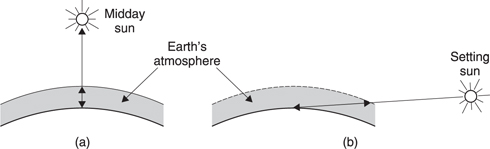
Although the radiation leaving the sun is relatively constant, the radiation arriving on Earth varies throughout the day. Figure 6.5(a) shows that at midday, the sun is high and the path through the atmosphere is short. The amount of scattering of the blue end of the spectum is minimal and the light has a blueish quality. However, at the end of the day, the sun is low and the path through the atmosphere is much longer as (b) shows. The extent of blue scattering is much greater and the remaining radiation reaching the observer becomes first orange as the sun gets low and finally red as it sets. Thus the colour temperature of sunlight is not constant. In addition to the factors mentioned, clouds will also change the colour temperature.
Light can also be emitted by atoms in which electrons have been raised from their normal, stable, orbit to one of higher energy by some form of external stimulus other than heat which could be ultra-violet light or electrical.
Electrons which fall back to the valence band emit a quantum of energy as a photon whose frequency is proportional to the energy difference between the bands. The process is described by Planck’s Law:
Energy difference E = H × f
where H = Planck’s Constant
= 6.6262 × 10⁻³⁴ Joules/Hertz
The wavelength of the light emitted is a function of the characteristics of a particular atom, and a great variety exist. The SPD of light sources of this kind is very narrow, appearing as a line in the spectrum. Some materials are monochromatic, whereas some have two or more lines. Useful and efficient illuminants can be made using mixtures of materials to increase the number of lines, although the spectrum may be far from white in some cases. Such illuminants can be given an effective colour temperature, even though there is nothing in the light source at that temperature. The colour temperature is that at which a black body and the illuminant concerned give the same perceived result to the HVS. This type of light generation is the basis of mercury and sodium lights, fluorescent lights, dayglo paint, the aurora borealis, whiteners in washing powder, phosphors in CRT and plasma displays, lasers and LEDs. It should be noted that although these devices have colour temperatures as far as the HVS is concerned, their line spectrum structure may cause them to have unnatural effects on other colour-sensitive devices such as film and TV cameras.
6.4 Optical principles
Wave theory of light suggests that a wavefront advances because an infinite number of point sources can be considered to emit spherical waves which will only add when they are all in the same phase. This can only occur in the plane of the wavefront. Figure 6.6 shows that at all other angles, interference between spherical waves is destructive. Note the similarity with sound propagation described in Chapter 5.

Figure 6.6 Plane-wave propagation considered as infinite numbers of spherical waves.
When such a wavefront arrives at an interface with a denser medium, such as the surface of a lens, the velocity of propagation is reduced; therefore the wavelength in the medium becomes shorter, causing the wavefront to leave the interface at a different angle (Figure 6.7). This is known as refraction. The ratio of velocity in vacuo to velocity in the medium is known as the refractive index of that medium; it determines the relationship between the angles of the incident and refracted wavefronts. Reflected light, however, leaves at the same angle to the normal as the incident light. If the speed of light in the medium varies with wavelength, dispersion takes place, where incident white light will be split into a rainbow-like spectrum leaving the interface at different angles. Glass used for chandeliers and cut glass is chosen to be highly dispersive, whereas glass for lenses in cameras and projectors will be chosen to have a refractive index which is as constant as possible with changing wavelength. The use of monochromatic light allows low-cost optics to be used as they only need to be corrected for a single wavelength. This is done in optical disk pickups and in colour projectors which use one optical system for each colour.

In natural light, the electric-field component will be in many planes. Light is said to be polarized when the electric field direction is constrained. The wave can be considered as made up from two orthogonal components. When these are in phase, the polarization is said to be linear. When there is a phase shift between the components, the polarization is said to be elliptical, with a special case at 90° called circular polarization. These types of polarization are contrasted in Figure 6.8.
In order to create polarized light, anisotropic materials are necessary. Polaroid material, invented by Edwin Land, is vinyl which is made anisotropic by stretching it while hot. This causes the long polymer molecules to line up along the axis of stretching. If the material is soaked in iodine, the molecules are rendered conductive, and short out any electric-field component along themselves. Electric fields at right angles are unaffected; thus the transmission plane is at right angles to the stretching axis.
Stretching plastics can also result in anisotropy of refractive index; this effect is known as birefringence. If a linearly polarized wavefront enters such a medium, the two orthogonal components propagate at different velocities, causing a relative phase difference proportional to the distance travelled. The plane of polarization of the light is rotated. Where the thickness of the material is such that a 90° phase change is caused, the device is known as a quarter-wave plate.

The action of such a device is shown in Figure 6.9. If the plane of polarization of the incident light is at 45° to the planes of greatest and least refractive index, the two orthogonal components of the light will be of equal magnitude, and this results in circular polarization. Similarly, circular-polarized light can be returned to the linear-polarized state by a further quarter-wave plate. Rotation of the plane of polarization is a useful method of separating incident and reflected light in a laser disk pickup.
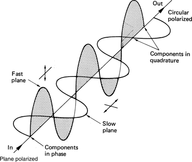
Figure 6.9 Different speed of light in different planes rotates the plane of polarization in a quarter-wave plate to give a circularly polarized output.
Using a quarter-wave plate, the plane of polarization of light leaving the pickup will have been turned 45°, and on return it will be rotated a further 45°, so that it is now at right angles to the plane of polarization of light from the source. The two can easily be separated by a polarizing prism, which acts as a transparent block to light in one plane, but as a prism to light in the other plane, such that reflected light is directed towards the sensor.
6.5 Photometric units
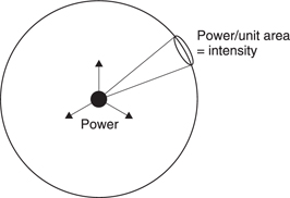
Radiometric and photometric units are different because the latter are affected by the luminous efficiency function of the eye. Figure 6.10 shows the two sets of units for comparison. Figure 6.11 shows an imaginary point light source radiating equally in all directions. An imaginary sphere surrounds the source. The source itself has a power output, measured in Watts, and this power uniformly passes through the area of the sphere, so the power per unit area will follow an inverse square law. Power per unit area is known as intensity, with units of Watts per square metre. Given a surface radiating with a certain intensity, viewed at right angles to the surface the maximum brightness would be measured. Viewed from any other angle the brightness would fall off as a cosine function.
The above units are indifferent to wavelength and whether the HVS can see the radiation concerned. In photometry, the equivalent of power is luminous flux, whose unit is the lumen, the equivalent of intensity is luminous intensity measured in candela and the equivalent of brightness is luminance measured in nits.

Figure 6.10 Radiometric and photometric units compared.
It is difficult to maintain a standard of luminous flux so instead the candela is defined. The candela replaced the earlier unit of candle power and is defined in such a way as to make the two units approximately the same. One square centimetre of platinum at its freezing point of 2042° K radiates 60 cd.
The lumen is defined as the luminous flux radiated over a unit solid angle by a source whose intensity is one candela. The nit is defined as one candela per square metre. As an example, a CRT may reach 200–300 nit.
In an optical system, the power of the source is often concentrated in a certain direction and so for a fixed number of candela the brightness in that direction would rise. This is the optical equivalent of forward gain in an antenna.
The lumen is a weighted value based on the luminous efficiency function of the HVS. Thus the same numerical value in lumens will appear equally bright to the HVS whatever the colour. If three sources of light, red, green and blue each of one lumen are added, the total luminous flux will be three lumens but the result will not appear white.
It is worth while discussing this in some detail. Figure 6.12(a) shows three monochromatic light sources of variable intensity which are weighted by the luminous efficiency function of the HVS in order correctly to measure the luminous flux. In order to obtain one lumen from each source, the red and blue sources must be set to produce more luminous flux than the green source. This means that the spectral distribution of the source is no longer uniform and so it will not appear white. In contrast, Figure 6.12(b) shows three sources which have the same luminous flux. After weighting by the luminous efficiency function, each source produces a different number of lumens, but the eye perceives the effect as white. Essentially the eye has a non-uniform response, but in judging colour it appears to compensate for that so that a spectrum which is physically white, i.e. having equal luminous flux at all visible wavelengths, also appears white to the eye.

As a consequence it is more convenient to have a set of units in which equal values result in white. These are known as tristimulus units and are obtained by weighting the value in lumens by a factor which depends on the response of the eye to each of the three wavelengths. The weighting factors add up to unity so that three tristimulus units, one of each colour, when added together produce one lumen. Tristimulus units will be considered further in section 6.14.
6.6 MTF, contrast and sharpness
All imaging devices, including the eye, have finite performance and the modulation transfer function (MTF) is a way of describing the ability of an imaging system to carry detail. The MTF is essentially an optical frequency response and is a function of depth of contrast with respect to spatial frequency. Prior to describing the MTF it is necessary to define some terms used in assessing image quality.
Spatial frequency is measured in cycles per millimetre (mm–1). Contrast Index (CI) is shown in Figure 6.13(a). The luminance variation across an image has peaks and troughs and the relative size of these is used to calculate the contrast index as shown. A test image can be made having the same Contrast Index over a range of spatial frequencies as shown in Figure 6.13(b). If a non-ideal optical system is used to examine the test image, the output will have a Contrast Index which falls with rising spatial frequency.

Figure 6.13 (a) The definition of contrast index (CI). (b) Frequency sweep test image having constant CI. (c) MTF is the ratio of output and input CIs.
The ratio of the output CI to the input CI is the MTF as shown in Figure 6.13(c). In the special case where the input CI is unity the output CI is identical to the output MTF. It is common to measure resolution by quoting the frequency at which the MTF has fallen to one half. This is known as the 50 per cent MTF frequency. The limiting resolution is defined as the point where the MTF has fallen to 10 per cent.
Whilst MTF resolution testing is objective, human vision is subjective and gives an impression we call sharpness. However, the assessment of sharpness is affected by contrast. Increasing the contrast of an image will result in an increased sensation of sharpness even though the MTF is unchanged. When CRTs having black areas between the phosphors were introduced, it was found that the improved contrast resulted in subjectively improved sharpness even though the MTF was unchanged. Similar results are obtained with CRTs having non-reflective coatings.
The perceived contrast of a display is also a function of the surroundings. Displays viewed in dark surroundings, such as cinema film and transparencies, appear to lack contrast whereas when the same technical contrast is displayed with light surroundings, the contrast appears correct. This is known as the surround effect. It can be overcome by artificially expanding the contrast prior to the display. This will be considered in section 6.9 where the subject of gamma is treated.
6.7 The human visual system
The HVS evolved as a survival tool. A species which could use vision to sense an impending threat, to locate food and a mate would have an obvious advantage. From an evolutionary standpoint, using the visual system to appreciate art or entertainment media is very recent. In a system having strong parallels to the hearing system described in Chapter 5, the HVS has two obvious transducers, namely the eyes, coupled to a series of less obvious but extremely sophisticated processes which take place in the brain. The result of these processes is what we call sight, a phenomenon which is difficult to describe.
At an average reading distance of 350 mm, the letters in this book subtend an angle to the eye of about a third of a degree. The lines from which the letters are formed are about one tenth of a millimetre across and subtend an angle of about one minute (one sixtieth of a degree). The field of view of the HVS is nearly a hemisphere. A short calculation will reveal how many pixels would be needed to convey that degree of resolution over such a wide field of view. The result is simply staggering. If we add colour and we also wish to update all those pixels to allow motion, it is possible to estimate what bandwidth would be needed.

The result is so large that it is utterly inconceivable that the nerves from the eye to the brain could carry so much data, or that the brain could handle it. Clearly the HVS does not work in this way. Instead the HVS does what the species finds most useful. It helps create a model in the mind of the reality around it.
Figure 6.14 shows the concept. The model can be considered like a kind of three-dimensional frame store in which objects are stored as the HVS identifies them. Inanimate objects are so called because they don’t move. They can be modelled once and left in the model until there is evidence to suggest that there has been a change. In contrast, animate objects need more attention, because they could be bringing benefit or detriment.
The HVS solves both of these requirements with the same mechanism. The eyes can swivel to scan the environment and their owner can move within it. This scanning process allows the model to be built using eyes with a relatively narrow field of view. Within this narrow field of view, the provision of high resolution and colour vision does not require absurd bandwidth, although it does require good lighting. Although the pixels are close together, the total number is fairly small.
Such narrow vision alone is not useful because events outside the field of vision do not alert the HVS to the need for an update of the model. Thus in addition there is a wider field of view which has relatively poor resolution and is colourblind, but which works at low light levels and responds primarily to small changes or movements.
Sitting at a laptop computer writing these words, I can only see a small part of the screen in detail. The rest of the study is known only from the model. On my right is a mahogany bracket clock, but in peripheral vision it appears as a grey lump. However, in my mind the wood and the brass are still the right colour. The ticking of the clock is coming from the same place in the model as the remembered object, reinforcing the illusion.
If I were to be replaced with a camera and a stereo microphone, and the two then turned to the right towards the clock, the visual image and the sound image would both move left. However, if I myself turn right this doesn’t happen. The signals from the balance organs in the ear, the sound image model and the visual model produce data consistent with the fact that it was I that moved and the result is that the model doesn’t move. Instead I have become another object in the model and am moving within it. The advantage of this detached approach is that my limbs are included in the model so that I can see an object and pick it up.
This interaction between the senses is very strong and disparities between the senses are a powerful clue that one is being shown an illusion. In advanced systems for use in electronic cinema or flight simulators, it is vital to maintain accurate tracking between the visual image, the sound image and the sense of balance. Disparities which are not obvious may often result in fatigue.
One consequence of seeing via a model is that we often see what we expect to see rather than what is before us. Optical illusions demonstrate this, and Maurits Escher turned it into an art form. The technique of camouflage destroys familiar shapes and confuses the modelling process. Animals and birds may freeze when predators approach because their lack of motion doesn’t trigger peripheral vision.
6.8 The eye
The simple representation of Figure 6.15 shows that the eyeball is nearly spherical and is swivelled by muscles. The space between the cornea and the lens is filled with transparent fluid known as aqueous humour. The remainder of the eyeball is filled with a transparent jelly known as vitreous humour. Light enters the cornea, and the the amount of light admitted is controlled by the pupil in the iris. Light entering is involuntarIly focused on the retina by the lens in a process called visual accommodation. The lens is the only part of the eye which is not nourished by the bloodstream and its centre is technically dead. In a young person the lens is flexible and muscles distort it to perform the focusing action. In old age the lens loses some flexibility and causes presbyopia or limited accommodation. In some people the length of the eyeball is incorrect resulting in myopia (short-sightedness) or hypermetropia (long-sightedness). The cornea should have the same curvature in all meridia, and if this is not the case, astigmatism results.
The retina is responsible for light sensing and contains a number of layers. The surface of the retina is covered with arteries, veins and nerve fibres and light has to penetrate these in order to reach the sensitive layer. This contains two types of discrete receptors known as rods and cones from their shape. The distribution and characteristics of these two receptors are quite different. Rods dominate the periphery of the retina whereas cones dominate a central area known as the fovea outside which their density drops off. Vision using the rods is monochromatic and has poor resolution but remains effective at very low light levels, whereas the cones provide high resolution and colour vision but require more light.

Figure 6.15 A simple representation of an eyeball; see text for details.
Figure 6.16 shows how the sensitivity of the retina slowly increases in response to entering darkness. The first part of the curve is the adaptation of cone or photopic vision. This is followed by the greater adaptation of the rods in scotopic vision. Figure 6.17 shows that the luminous efficiency function is different for scotopic vision, peaking at around 507 nm. This is known as the Purkinje effect. At such low light levels the fovea is essentially blind and small objects which can be seen in the peripheral rod vision disappear when stared at. A significant area of the retina, where the optic nerve connects, is completely blind. However we are not aware of a hole in our vision because we don’t see the image on the retina literally. Instead we see the visual model which inserts information in the hole. The hole is in a different place in each eye which assists in this concealment process.
The cones in the fovea are densely packed and directly connected to the nervous system allowing the highest resolution. Resolution then falls off away from the fovea. As a result the eye must move to scan large areas of detail. The image perceived is not just a function of the retinal response, but is also affected by processing of the nerve signals. The overall acuity of the eye can be displayed as a graph of the response plotted against the degree of detail being viewed. Detail is generally measured in lines per millimetre or cycles per picture height, but this takes no account of the distance from the eye. A better unit for eye resolution is one based upon the subtended angle of detail as this will be independent of distance. Units of cycles per degree are then appropriate. Figure 6.18 shows the response of the eye to static detail. Note that the response to very low frequencies is also attenuated. An extension of this characteristic allows the vision system to ignore the fixed pattern of shadow on the retina due to the nerves and arteries.

Figure 6.16 Retinal sensitivity changes after sudden darkness. The initial curve is due to adaptation of cones. At very low light levels cones are blind and monochrome rod vision takes over.

Figure 6.17 The luminous efficiency function is different for scotopic vision.
The resolution of the eye is primarily a spatio-temporal compromise. The eye is a spatial sampling device; the spacing of the rods and cones on the retina represents a spatial sampling frequency and the finite area of the individual sensors results in an aperture effect. However, if these parameters are measured and an MTF is estimated, it will be found that the measured acuity of the eye exceeds the value calculated.

Figure 6.18 The response of the eye to static detail falls off at both low and high spatial frequencies.
This is possible because a form of oversampling is used. Figure 6.19 shows that the eye is in a continuous state of unconscious vibration called saccadic motion. This causes the sampling sites to exist in more than one location, effectively increasing the spatial sampling rate provided there is a temporal filter which is able to integrate the information from the various different positions of the retina.
This temporal filtering is partly responsible for persistence of vision and other effects. The HVS does not respond instantly to light, but requires between 0.15 and 0.3 second before the brain perceives an image, although that image could have been presented for an extremely short length of time. At low light levels the time taken to perceive an image increases. The position of moving objects is perceived with a lag which causes the geometry of stereoscopic depth perception to be in error, a phenomenon known as the Pulfrich effect.
Scotopic vision experiences a greater delay than photopic vision as more processes are required. Images are retained for about 0.1 second. Flashing lights are perceived to flicker until the critical flicker frequency is reached, when the light appears continuous for higher frequencies. Figure 6.20 shows how the CFF changes with brightness. The CFF in peripheral vision is higher than in foveal vision. This is consistent with using peripheral vision to detect movement.

Figure 6.19 The eye is constantly moving and this causes the sampling sites on the retina to exist in more places, enhancing resolution.

Figure 6.20 The critical flicker frequency is not constant but rises as brightness increases.
The critical flicker frequency is also a function of the state of alertness of the individual. When people are tired or under stress, the rate at which the brain updates the model appears to slow down so that the CFF falls.1
The response of the eye is effectively two-dimensional as it is affected by spatial frequencies and temporal frequencies. Figure 6.21 shows the two-dimensional or spatio-temporal response of the eye. If the eye were static, a detailed object moving past it would give rise to temporal frequencies, as Figure 6.22(a) shows. The temporal frequency is given by the detail in the object, in lines per millimetre, multiplied by the speed. Clearly a highly detailed object can reach high temporal frequencies even at slow speeds, and Figure 6.21 shows that the eye cannot respond to high temporal frequencies; a fixed eye cannot resolve detail in moving objects. The solution is that in practice the eye moves to follow objects of interest. Figure 6.22(b) shows that when the eye is following an object the image becomes stationary on the retina and the temporal frequencies are brought to zero. The greatest resolution is then possible. Clearly whilst one object is being followed other objects moving differently will be blurred. This ability of the eye to follow motion has a great bearing on the way that discrete frames are perceived as a continuously moving picture and affects the design of motion-compensated equipment. This will be discussed further in section 6.10.

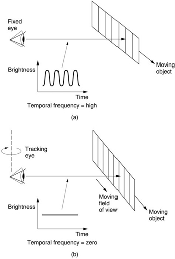
Figure 6.22 In (a) a detailed object moves past a fixed eye, causing temporal frequencies beyond the response of the eye. This is the cause of motion blur. In (b) the eye tracks the motion and the temporal frequency becomes zero. Motion blur cannot then occur.
6.9 Gamma
Gamma is the power to which the voltage of a conventional analog video signal must be raised to produce a linear light representation of the original scene. At the bottom of it all, there are two reasons for gamma. One is the perennial search for economy and the other is a characteristic of the human visual system which allows the economy to be made. The truth is that gamma is a perceptive compression system. It allows a television picture of better perceived quality to pass through a signal path of given performance.
The true brightness of a television picture can be affected by electrical noise on the video signal. The best results will be obtained by considering how well the eye can perceive such noise. The contrast sensitivity of the eye is defined as the smallest brightness difference which is visible. In fact the contrast sensitivity is not constant, but increases proportionally to brightness. Thus whatever the brightness of an object, if that brightness changes by about 1 per cent it will be equally detectable.
If video signals were linear, at maximum brightness the signal would have to be a hundred times bigger than the noise. However, if the signal were half as bright, the noise level would also have to be halved, so the SNR would now have to be 6 dB better. If the signal were one tenth as bright, a noise level ten times lower would be needed. The characteristic of the eye means that noise is more visible in dark picture areas than in bright areas.
For economic reasons, video signals have to be made non-linear to render noise less visible. An inverse gamma function takes place on the linear light signal from the camera so that the video signal is non-linear for most of its journey. Figure 6.23 shows a typical inverse gamma function. As a true power function requires infinite gain near black, a linear segment is substituted. Where it is necessary to compensate for the surround effect (see section 6.6) the gamma and inverse gamma processes can be made slightly different so that an overall non-linearity results. This improves perceived contrast when viewing in dark surroundings.
The result of using gamma is that contrast variations in the original scene near black result in a larger signal amplitude than variations near white. The result is that noise picked up by the video signal has less effect on dark areas than on bright areas, countering the sensitivity of the eye. After a gamma function at the display, noise at near-black levels is compressed with respect to noise near-white levels. Thus a video transmission system using gamma has a lower perceived noise level than one without. Without gamma, vision signals would need around 30 dB better signal-to-noise ratio for the same perceived quality and digital video samples would need five or six extra bits.
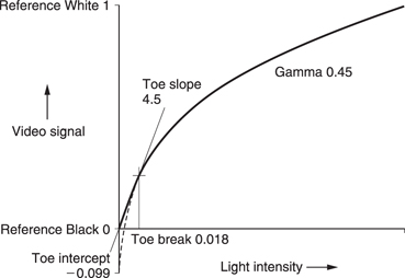
Figure 6.23 CCIR Rec. 709 inverse gamma function used at camera has a straight line approximation at the lower part of the curve to avoid boosting camera noise. Note that the output amplitude is greater for modulation near black.
There is a strong argument to retain gamma in the digital domain for analog compatibility. In the digital domain transmission noise is eliminated, but instead the conversion process introduces quantizing noise.
As all television signals, analog and digital, are subject to gamma correction, it is technically incorrect to refer to the Y signal as luminance, because this parameter is defined as linear in colorimetry. Charles Poynton2 has suggested that the term luma should be used to describe the signal which results when luminance has been gamma corrected so that it is clear that a non-linear signal is being considered. That convention has been adopted throughout this book.
Figure 6.24 shows that digital luma can be considered in several equivalent ways. At (a) a linear analog luminance signal is passed through a gamma corrector to create luma and this is then quantized uniformly. At (b) the linear analog luminance signal is fed directly to a non-uniform quantizer. At (c) the linear analog luminance signal is uniformly quantized to produce digital luminance. This is converted to digital luma by a digital process having a non-linear transfer function.
Whilst the three techniques shown give the same result, (a) is the simplest, (b) requires a special ADC with gamma-spaced quantizing steps, and (c) requires a high-resolution ADC of perhaps fourteen to sixteen bits because it works in the linear luminance domain where noise is highly visible. Technique (c) is used in digital processing cameras where long wordlength is common practice.
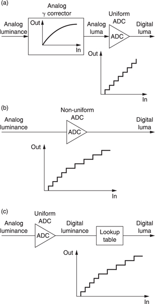
Figure 6.24 (a) Analog γ correction prior to ADC. (b) Non-uniform quantizer gives direct γ conversion. (c) Digital γ correction using look-up table
As digital luma with eight-bit resolution gives the same subjective performance as digital luminance with fourteen-bit resolution it will be clear why gamma can also be considered as a perceptive compression technique.
As gamma is derived from a characteristic of the eye, there is only one correct value, which is the one that gives an apparent sensitivity to noise which is independent of brightness. Too little gamma and we would see more noise in dark areas. Too much and we would see more noise in highlights. This is why it is regarded as a constant in television. All the more surprising that in computer graphics standards gamma varies considerably. As the use of computers in television spreads, this incompatibility can be a source of difficulty.
Clearly image data which are intended to be displayed on a television system must have the correct gamma characteristic or the grey scale will not be correctly reproduced. Image data from computer systems often have gamma characteristics which are incompatible with the standards adopted in video and a gamma conversion process will be required to obtain a correct display. This may take the form of a lookup table or an algorithm.
So what has gamma got to do with CRTs? The electrons emitted from the cathode have negative charge and so are attracted towards an anode which is supplied with a positive voltage. The voltage on the grid controls the current. The electron beam strikes the inside of the tube face which is coated with phosphor. The intensity of the light produced is effectively controlled by the intensity of the electron beam which is in turn controlled by the grid voltage. It is the relative voltage between the cathode and the grid which determines the beam current.
The relationship between the tube drive voltage and the phosphor brightness is not linear, but is an exponential function. The power is the same for all CRTs as it is a function of the physics of the electron gun and it has a value of around 2.8. It is a happy but pure coincidence that the gamma function of a CRT follows roughly the same curve as human contrast sensitivity.

Figure 6.25 The non-linear characteristic of tube (a) contrasted with the ideal response (b). Non-linearity may be opposed by gamma correction with a response (c).
Consequently if video signals are pre-distorted at source by an inverse gamma, the gamma characteristic of the CRT will linearize the signal. Figure 6.25 shows the principle. CRT non-linearity is actually used to enhance the noise performance of a television system. If the CRT had no gamma characteristic, a gamma circuit would have been necessary ahead of it to linearize the gamma-corrected video signals. As all standard video signals are inverse gamma processed, it follows that if a non-CRT display such as a plasma or LCD device is to be used, some gamma conversion will be required at the display. In a plasma display, the amount of light emitted is controlled by the duration of the discharge and a voltage-topulse- length stage is needed in the drive electronics. It is straightforward to include a gamma effect in this conversion.
6.10 Motion portrayal and dynamic resolution
Althought the term ‘motion pictures’ is commonly used, it is inaccurate. Today’s film, television and graphics systems do not present moving pictures at all. Instead they present a series of still pictures at a frequency known as the frame rate. The way that the human visual system interprets periodically updated still pictures to obtain an illusion of motion has only been put on a scientific basis relatively recently. Most of today’s imageportrayal systems were designed empirically before this knowledge was available and it is hardly surprising that in the absence of a theory the results are often poor and myth abounds.
All high-quality non-stereoscopic image-portrayal systems should look the same to the viewer as the original scene when viewed through one eye. This must hold not only for the appearance of any objects but also for their motion. At the time of writing this cannot be said for film or television, which differ obviously from one another and from the original scene.
To suggest that re-creation of the original scene is the only acceptable goal is pedantic as this is probably not necessary. However, it can fairly be stated that the standards of realism of present-day systems are somewhat lacking and a degree of improvement is desirable, particularly in the portrayal of motion. That improvement is not especially difficult with modern technology as will be shown here.
As was shown in section 6.7, the eye uses involuntary tracking at all times. This means that the criterion for comparing moving imageportrayal systems has to be the apparent resolution perceived by the viewer in an object moving within the limits of accurate eye tracking. The traditional metric of static resolution in film and television has to be abandoned as unrepresentative of the viewing experience and replaced with a more appropriate metric known as dynamic resolution.

Figure 6.22(b) showed an eye tracking a real detailed moving object. The tracking process renders the object stationary with respect to the retina and so the eye can perceive detail. Figure 6.26 shows the eye tracking the same object, but this time on the screen of an image-portrayal system. The camera and display are fixed. This results in high temporal frequencies being present in the imaging system.
Consider an example of a moving object containing moderate detail of 80 cycles per picture width. If the object moves at a speed of one picture width per second, the temporal frequency due to the object modulation moving past a given pixel in the fixed camera is 80 Hz. In conventional systems, this temporal frequency is sampled at the frame rate, typically only 24, 25 or 30 Hz. According to conventional sampling theory, this is a recipe for aliasing, whereas film and television are known to work reasonably well. One may be forgiven for wondering what is going on and the explanation is based on the fact that eye tracking has a dramatic effect.
Figure 6.27 shows that when the moving eye tracks an object on the screen, the viewer is watching with respect to the optic flow axis, not the time axis, and these are not parallel when there is motion. The optic flow axis is defined as an imaginary axis in the spatio-temporal volume which joins the same points on objects in successive frames. Clearly when many objects move independently there will be one optic flow axis for each, although the HVS can only track one at a time.


Figure 6.28 A real moving object contains a range of spatial frequencies. The low frequencies allow eye tracking to be performed, and once the eye is tracking correctly, the aliased high frequencies are hetererodyned back to their correct baseband frequency so that detail can be seen in moving areas.
Figure 6.28(a) shows that real scenes contain many spatial frequencies rather than hypothetical sine waves. The bulk of an object is carried in low spatial frequencies and the temporal frequency due to motion is quite low and does not alias. This allows the eye to track a moving object. When the eye is tracking, it views the series of presented pictures along the optic flow axis. Figure 6.28(b) shows that this eye tracking arrests the temporal frequency due to moving detail, allowing the spatial detail to be seen. Note that aliasing occurs on the time axis, but this is not seen by the tracking eye. It is only eye tracking which allows the use of such low picture rates. However well low picture rates work on the tracked object, it is important to consider what happens on parts of the picture which are not being tracked.
It is a further consequence of Figure 6.28(a) that the observer perceives the direction of motion of an object before the object can be seen in detail. The detail can only be seen when the eye has achieved tracking.
When the eye is tracking, successive pictures appear in different places with respect to the retina. In other words if an object is moving down the screen and followed by the eye, the screen, and the background image portrayed on it, is actually moving up with respect to the retina.
6.11 Background strobing and frame rate
In real-life eye tracking, the motion of the background will be smooth, but in an image-portrayal system based on periodic presentation of frames, the background will be presented to the retina in a different position in each frame. The retina separately perceives each impression of the background leading to an effect called background strobing which is shown in Figure 6.29.
The criterion for the selection of a display frame rate in an imaging system is sufficient reduction of background strobing. It is a complete myth that the display rate simply needs to exceed the critical flicker frequency. Manufacturers of graphics displays which use frame rates well in excess of those used in film and television are doing so for a valid reason: it gives better results! Note that the display rate and the transmission rate need not be the same in an advanced system. The picture rate may artificially be increased prior to display.
6.12 Colour
There are many aspects of colour to consider in imaging systems. It is conventional to begin with colour science which explains what is happening both in physics and in the eye, as this will define the problem of colour portrayal. Ideally a sensor with at least the same colour acuity as the eye would be used to create colour data whose transmission is probably the easiest part of the system. An ideal display would be able to re-create the original colours.
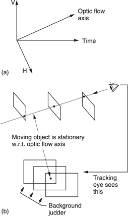
Figure 6.29 The optic flow axis (a) joins points on a moving object in successive pictures. (b) When a tracking eye follows a moving object on a screen, that screen will be seen in a different place at each picture. This is the origin of background strobing.
Practicality and economics mean that ideal colour reproduction is seldom achieved in real systems, primarily because of difficulties in the display, but nevertheless good results can be obtained with a little care. The approach of this chapter will be to describe current practice, but without losing sight of the fact that improvements are possible. As convergence continues, it will increasingly become important for colour data to be transferable between previously separate disciplines. Computer data representing a coloured image may be used to drive a CRT display, a colour printer or a film recorder or to make plates for a press. In each case the same colours should be obtained as on the computer monitor. At the moment the disparity of technologies makes such transfers non-trivial.
6.13 Colour vision
When considering everyday objects at normal temperatures, the blackbody radiation is negligible compared to the reflection of ambient light. Figure 6.30 shows that the colour perceived by the human observer is a function of the illuminant and the reflectivity of the object concerned.
The sensation of colour is entirely a fabrication of the human visual system and in the real world there is only a distribution of energy at different wavelengths. There is no fixed relationship between the two. The SPD of daylight varies throughout the day, and the SPD of many artificial light sources is different again. As a result the SPD reaching the eye in the reflection from some object is subject to a lot of variation. However, although this ought to cause things to change colour, this is not what we see. It would cause enormous practical difficulties if we saw ‘true’ colour. Imagine parking a white car at midday and being unable to locate it just before sunset because it has become red.
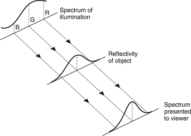
Figure 6.30 The spectrum of the light perceived by the HVS is a function of the spectrum of the illumination and the reflectivity of the object concerned. Thus it is incorrect to state that colour is a property of an object as this assumes a certain type of lighting.
Instead the HVS compensates so that we can recognize our property and our friends despite changes in natural or artificial illumination. In the absence of any reference, the eye automatically tries to colour balance an image so that familiar objects in it have familiar colours.
This characteristic of seeing the colour we expect means that the absolute accuracy of colour reproduction can be fairly poor. However, the differential accuracy of colour vision is astonishingly good. If during the filming of a movie or TV program, footage shot at midday is edited onto footage shot later on, the sudden jump of colour balance will be obvious to all. Film and TV cameras don’t have the subconscious colour corrector of the HVS and steps have to be taken artificially to maintain the same colour balance. Another example of differential colour accuracy is the difficulty of matching paint on replacement car body panels.
The eye is able to distinguish between different SPDs because it has sensors in the retina called cones which respond in three different ways. Each type of cone has a different spectral response curve. The rods in the retina which operate at extremely low light levels only exist in one type and so there is no colour vision when the rods are in use. The full resolution of human vision is restricted to brightness variations. Our ability to resolve colour details is only about a quarter of that.
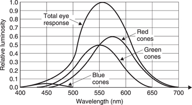
Figure 6.31 The approximate response of each type of cone in the retina.
Figure 6.31 shows an approximate response for each of the three types of cone. If light of a single wavelength is observed, the relative responses of the three sensors allows us to discern what we call the colour of the light. Note that at both ends of the visible spectrum there are areas in which only one receptor responds; all colours in those areas look the same. There is a great deal of variation in receptor response from one individual to the next and the standard curves used in colorimetry are not necessarily valid for an individual. In a surprising number of people the single receptor zones are extended and discrimination between, for example, red and orange is difficult.
The responses of Figure 6.31 are broad and this means that a considerable range of SPDs actually appear to have the same colour. The eye will perceive, for example, the same white sensation whether the light has flat SPD or whether it consists of three monochromatic components. Maxwell’s triangle (Figure 6.32) was an early attempt to depict the operation of the eye graphically.
The HVS appears to average the SPD of the light it is analysing in two dimensions. The result of additively mixing any two colours will appear on a straight line between them at a location which is a function of the relative intensity. Thus adding red and green will create yellow, and in turn yellow and blue will create white. It does not matter whether the yellow is spectral yellow or whether it is a mixture of red and green. These effects are summarized by Grassman’s Law: sources of the same colour produce identical effects in a mixture regardless of their spectral composition.

Figure 6.32 Maxwell’s triangle was an early attempt at understanding colour vision.
As a result it is possible for somewhat different SPDs to be perceived as exactly the same colour. Such SPDs are known as metamers. Figure 6.33 shows some metamers. White light as perceived by the HVS can be spectrally uniform, a mixture of red and cyan or equal parts of red, green and blue, or an infinite number of such variations.
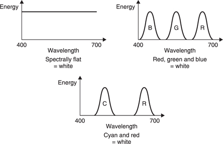
Figure 6.33 Metamers are spectral distributions which appear the same colour to the HVS.
Metamerism is both good and bad. It is good because it allows colourimaging equipment to be much simpler than otherwise. However, it is bad because it allows illuminants which are metamers of white but which are anything but spectrally uniform. An example is fluorescent light which appears white but makes coloured objects appear different because the narrow line spectra may not coincide with the reflectivity function of the object concerned. Try looking at mahogany in daylight and then under fluorescent light. This effect also plays havoc with colour film which is not expecting narrow spectra and will suffer strong colour casts, generally towards green which does nothing for flesh tones.
6.14 Colorimetry
The triple receptor or trichromatic characteristic of the eye is extremely fortunate as it means that it is possible to represent the full range of visible colours and brightness by only three signals. However, this is only true if the three signals are obtained in an appropriate way. It does not follow that it is possible to re-create the entire visible colour range with only three different light sources, and this distinction will be clarified here. Nevertheless with three sources a large range of colours is still possible. It is important to appreciate that some colours occur very rarely and the inability accurately to re-create them in systems designed for entertainment is not serious. However, for technical or security purposes it may be an issue.
There are two ways of creating colours, which amount to alternative ways of producing the same SPD. One can start with a wide spectrum such as white light and narrow it down by removing part of the spectrum with filters, or one can create weighted amounts of light at three discrete wavelengths which are added up. Cinema film operates on the former principle, known as subtractive colour matching, whereas colour CRTs operate on the latter, known as additive colour matching. Subtractive colour matching also occurs with paints and inks.
Colour is subjective and it is difficult to describe a colour accurately without an objective basis. The work on objective measurement of colour vision was carried out by the Commission Internationale d’Eclairage (CIE) in the 1920s.
The CIE chose three monochromatic primaries, 436 and 546 nm from mercury lamps and 700 nm from a neon lamp. Once the primaries have been selected, the proportions needed to reproduce a given colour can be found, and from these proportions it will be possible to specify the spectral characteristics of the three analysis filters needed to produce three signals representing the colours. These analysis filters are called CIE colour matching functions.

Figure 6.34 Simple colorimeter. Intensities of primaries on the right screen are adjusted to match the test colour on the left screen.
Figure 6.34 shows a colorimeter used for finding colour matching functions. It consists of two adjacent white screens. One screen is illuminated by three light sources, one of each of the primary colours selected for the system being designed. Initially, the second screen is illuminated with white light and the three sources are adjusted until the first screen displays the same white. This calibrates the sources. Light of a single wavelength is then projected on the second screen. The primaries are once more adjusted until both screens appear to have the same colour. The proportions of the primaries are noted.

Figure 6.35 Colour mixture curves show how to mix primaries to obtain any spectral colour.

This process is repeated for the whole visible spectrum, resulting in colour mixture curves or tristimulus values shown in Figure 6.35.
In some cases it was found impossible to find a match. Figure 6.36 shows that the reason for the inability to match is that Maxwell’s triangle in an incomplete description of colour vision. In fact the colours which can be perceived go outside the triangle, whereas the colour which can be created must reside within it. For example, if it is attempted to match pure cyan at a wavelength of 490 nm, this cannot be approached more closely than the limit set by the line between green and blue, which corresponds to the red source being turned off completely.
For analysis purposes a negative contribution can be simulated by shining some primary colour on the test screen until a match is obtained. The colour mixing curves dictate what the spectral response of the three sensors must be if distinct combinations of three signals are to be obtained for all visible colours.
6.15 The CIE chromaticity diagram
As there are three variables, they can only simultaneously be depicted in three dimensions. Figure 6.37 shows the RGB colour space which is basically a cube with black at the origin and white at the diagonally opposite corner. Figure 6.38 shows the colour mixture curves of Figure 6.35 plotted in RGB space. For each visible wavelength a vector exists whose direction is determined by the proportions of the three primaries. If the brightness is allowed to vary this will affect all three primaries and thus the length of the vector in the same proportion.
Depicting and visualizing the RGB colour space is not easy and it is also difficult to take objective measurements from it. The solution is to modify the diagram to allow it to be reproduced in two dimensions on flat paper.

Figure 6.37 RGB colour space is three-dimensional and not easy to draw.

Figure 6.38 Colour mixture curves plotted in RGB space result in a vector whose locus moves with wavelength in three dimensions.
This is done by eliminating luminance (brightness) changes and depicting only the colour at constant brightness. Figure 6.39(a) shows how a constant luminance unit plane intersects the RGB space at unity on each axis. At any point on the plane the three components add up to one. A two-dimensional shape results when vectors representing all colours intersect the plane. Vectors may be extended if necessary to allow intersection. Figure 6.39(b) shows that the 500 nm vector has to be produced (extended) to meet the unit plane, whereas the 580 nm vector naturally intersects. Any colour can now uniquely be specified in two dimensions.
The points where the unit plane intersects the axes of RGB space form a triangle on the plot. The horseshoe-shaped locus of pure spectral colours goes outside this triangle because, as was seen above, the colour mixture curves require negative contributions for certain colours.
Negative values are a nuisance and can be eliminated by new coordinates called X, Y and Z. Figure 6.39(c) shows that in this representation the origin is in the same place for XYZ and RGB, but the RGB axes have been turned inwards just far enough that the spectrum locus does not extend beyond the YZ, YX or ZX planes. Thus at about 570 nm the spectrum locus touches y = 1 – x and at about 500 nm it touches Y = 1 – Z and so on.

Figure 6.39 (a) A constant luminance plane intersects RGB space, allowing colours to be studied in two dimensions only. (b) The intersection of the unit plane by vectors joining the origin and the spectrum locus produces the locus of spectral colours which requires negative values of R, G and B to describe it.
The CIE standard chromaticity diagram shown in Figure 6.39(d) is obtained in this way by projecting the unity luminance plane onto the X, Y plane. As luminance has been eliminated by making x + y + z = 1, one of these parameters is redundant to describe the colour. By projecting onto the XY plane, the Z axis is the one which is made redundant. As a result only two trichromatic coefficients, x and y, are needed to convey all possible colours.

Figure 6.39 (Continued) In (c) a new coordinate system, X, Y, Z, is used so that only positive values are required. The spectrum locus now fits entirely in the triangular space where the unit plane intersects these axes. To obtain the CIE chromaticity diagram (d), the locus is projected onto the X–Y plane.
It is worth spending some time considering the CIE chromaticity diagram. The curved part of the locus is due to spectral or monochromatic colours over the visible range. The straight base is due to nonspectral colours obtained additively by mixing red and blue. Note that this base is not parallel to the X-axis because the R axis has been turned. It should be clear from Figure 6.40 that because there is a large cyan area outside the primary triangle, a corresponding quantity of ‘negative red’ is needed to match it. This results in a significant tilt of the R axis being needed to prevent negative values of r going below the ZX plane.
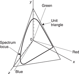
Figure 6.40 The RGB axes of Figure 6.37 are no longer orthogonal in CIE colour space. As shown here, the axes are turned inward sufficiently that no valid combination of R, G and B results in negative values of X,Y or Z.
Although the development of the CIE diagram has been traced starting from a stated set of primaries, it would not make any difference if the tests had been done with another set. For example, if a monochromatic source at 500 nm had been available, Figure 6.41 would apply. There would be a large set of yellows outside the primary triangle and this would have resulted in a large amount of ‘negative blue’ being needed to match. Thus the (different) RGB axes would still have to be turned in just enough to make them non-negative in XYZ space and this would have resulted in the same diagram.
Although colour is subjective, the independence of the CIE colour diagram from the primaries used to measure it makes it about as objective a tool as there is likely to be. Only colours within the the curve and its straight base exist. Combinations of x and y outside this area are invalid and meaningless. Valid combinations of x and y will be interpreted as the same colour by anyone who has access to the CIE document.

The projection chosen has the effect of bringing the red and blue primaries closer together than they are in the x + y + z = 1 plane. Thus the main drawback is that equal distances on the diagram do not correspond to equal subjective changes. The distance on the diagram between equal increments of wavelength are greater near the Y axis than elsewhere.
Whites appear in the centre of the chromaticity diagram corresponding to roughly equal amounts of primary colour (x = y = z = 0.333 …). More will be said about whites in due course. Two terms are used to describe colours: hue and saturation. Colours having the same hue lie on a straight line between the white point and the perimeter of the primary triangle. The saturation of the colour increases with distance from the white point. As an example, pink is a desaturated red. A saturated, or spectral, colour is monochromatic and has a single line spectrum. Desaturation results in an increasing level of energy at all other wavelengths

Figure 6.42 (a) The end-weighted spectrum perceived as purple. (b) The flat spectrum perceived as white. (c) The centre weighted spectrum perceived as green.
The peak photopic response of the eye at 550 nm is where the curve touches the line of y = 1 – x at y = 0.666 …, x = 0.333. As white has the same x coordinate, the complementary colour to peak green must be where x = 0.333 … crosses the non-spectral base line. It is useful to consider what happens on ascending this line from purple to green. Figure 6.42(a) shows that on the non-spectral line purple results from significant levels of red and blue but no green. This makes the spectrum end-weighted as shown. Figure 6.42(b) shows that white is due to equal amounts of primary, making the spectrum flat (literally white). Figure 6.42(c) shows that green is due to a centre-weighted spectrum.
6.16 Whites
Whites occupy the centre of the chromaticity diagram. As colour is subjective, there is no single white point. The closest to objectivity that is possible is CIE illuminant E which is defined as having uniform power through the visible spectrum. This corresponds to x = y = z = 0.3333 … Figure 6.43 shows the location of various ‘white’ sources or illuminants on the chromaticity diagram. Illuminant A corresponds to the SPD of a tungsten filament lamp having a colour temperature of 3200°K and appears somewhat yellow. Illuminant B corresponds to midday sunlight and illuminant C corresponds to typical daylight which is bluer because it consists of a mixture of sunlight and light scattered by the atmosphere. Illuminants B and C are effectively obsolete and have been replaced by the D series of illuminants which represent various types of daylight. D65 is the closest approximation to typical daylight. Colour systems which generate their own light, such as electronic displays, should use D65 white. In applications such as colour photographs and printing, the illumination under which the images will be viewed is out of the manufacturer’s control. This could be daylight or artificial light and the D50 and D55 illuminants represent a compromise between natural and tungsten light.

Figure 6.43 Position of various illuminants on the CIE diagram.
Computer monitors are often used in high ambient lighting levels which requires a bright display. Many computer images are entirely synthetic and colour accuracy is of little consequence. As practical blue phosphors are more efficient than red and green phosphors, it is easy to increase the brightness of a display by incorporating more blue. This leads to a colour temperature of about 9300°K. This is fine for generalpurpose computing but of no use at all for colour-imaging work. In this case the monitor will have to be recalibrated by turning down the blue drive signal.
6.17 Colour matching functions
The CIE chromaticity diagram eliminates brightness changes by considering only x and y. In a real sensing device, measuring x, y and z would allow brightness to be measured as well as the colour. Such a sensor must have three sensing elements, each having a different filtering effect or sensitivity with respect to wavelength. These filter specifications are known as colour matching functions which must be consistent with the derivation of the CIE diagram. In fact the way the CIE diagram is designed makes one of the colour matching functions, y, take the shape of the luminous efficiency function. Effectively y has the same spectral response as a monochrome camera would need in order to give the correct brightness for objects of any colour. The addition of x and z allow the hue and saturation of an object to be conveyed.
Figure 6.44 shows some examples of how the colour matching functions follow from the CIE diagram. It must be recalled that the valid region of the diagram is actually a projection of a plane given by x + y + z = 1. Thus for any spectral colour on the CIE diagram, the necessary values of x and y can be read off and the value of z can be calculated by a simple subtraction from 1. Plotting x, y and z against wavelength gives the shape of the colour matching functions. These are then normalized so that at the peak of the y response the distribution coefficient has a value of unity.

Note that the three colour matching functions are positive only and so it is technically possible to make a three-sensor camera equipped with filters having these functions which can capture every nuance of colour that the HVS can perceive in the three output signals.
It does not follow that a display can be made having three light sources to which these signals are directly connected. The primaries necessary accurately to produce a display directly from xyz tristimuli cannot be implemented because they are outside the valid region of the colour diagram and do not exist.
6.18 Choice of primaries
In order to produce all possible colours, the CIE xyz tristimulus signal would have to control a display which was capable of generating a colour anywhere within the valid region of the chromaticity diagram. Strictly this would require tunable light sources which could produce monochromatic light at any visible wavelength. These are not commercially available and instead the most common solution is to provide only three primary colours loosely called red, green and blue, which are not necessarily monochromatic. Only colours within the triangle joining the primaries can be reproduced and clearly efforts should be made to obtain primaries which embrace as large an area as possible. Figure 6.45 shows how the colour range or gamut of television compares with paint and printing inks and illustrates that the comparison is favourable. Most everyday scenes fall within the colour gamut of television. Exceptions include saturated turquoise, spectrally pure iridescent colours formed by interference in duck’s feathers or reflections in Compact Discs. For special purposes displays have been made having four primaries to give a wider colour range, but these are uncommon.
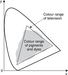
Figure 6.45 Comparison of the colour range of television and printing.
Figure 6.46 shows the primaries initially selected for NTSC. However, manufacturers looking for brighter displays substituted more efficient phosphors having a smaller colour range. This was later standardized as the SMPTE C phosphors using CIE D65 white. These were also adopted for PAL as ITU Rec. 709. In principle, the use of lasers as primaries is beneficial because they produce monochromatic light which, by definition, must be on the perimeter of the CIE diagram.
Once the primaries have been selected from those available, the next step is to determine how they can be driven. In principle, the CIE xyz tristimuli can be converted into primary drive signals using a suitable signal processor programmed with the necessary geometry. For any xyz triple, a given location on the chromaticity diagram would be addressed and this could be converted to the appropriate combinations of RGB. This is only possible within the triangle formed by the primaries. Outside the triangle the mathematically correct result would be that one or more of the RGB signals would be negative, but as this is non-realizable, they would simply be clipped to zero.

Figure 6.46 The primary colours for NTSC were initially as shown. These were later changed to more efficient phosphors which were also adopted for PAL. See text.
It is possible to conceive of a display having more than three primaries which would offer a wider colour gamut. In this case the signal processor would convert the CIE xyz tristimuli into any convenient metamer of the true colour. In other words over a large part of the chromaticity diagram there will be more than one combination of four or more primaries which would give the same perceived result. As the primaries are approached, the possibility for metamerism falls.
The advantage of using the CIE xyz analysis functions is that the full colour gamut is inherent in the video signal and any recordings made of it. The visible gamut is limited only by the available display. If in the future displays with wider gamut become economic, existing video recordings would be displayed more realistically.
In traditional colour television systems this approach has not been taken. Television was perceived as an entertainment medium in which strict accuracy was not needed and the high cost of implementing CIE colour matching functions in cameras to produce accurate signals could not be justified if the accuracy could not be displayed. Thus for technical purposes conventional television cameras may be unsuitable.
Instead, traditional television cameras use colour matching functions which are easy to implement and compatible with the limited gamut of the standardized phosphors. Certain colours are not theoretically reproduceable, and those colours that are reproduced are often distorted to some extent. The approach used in television will be considered in Chapter 7.
References
1. Hosokawa, T., Mikami, K. and Saito, K., Basic study of the portable fatigue meter: effects of illumination, distance from eyes and age. Ergonomics, 40, 887–894 (1997)
2. Poynton, C., A Technical Introduction to Digital Video, New York: John Wiley (1996)