
1
Introduction to convergent systems
1.1 What this book is about
The range of products and services which can be based on various combinations of audio, video and computer technology is limited only by the imagination. From the musical greetings card through videophones, digital photography, MP3 players, Internet video and video-on-demand to flight simulators, electronic cinema and virtual reality, the same fundamentals apply. The wide scope of this book has made it essential to establish some kind of order.
The purpose of this chapter is to show why binary coding and digital processing are so powerful, to introduce a number of key concepts and to give some examples of convergent systems and their far-reaching consequences. The explanations of this chapter are deliberately brief to avoid obscuring the overall picture with too much detail. Instead it will be indicated where in the book the in-depth treatment can be found. Figure 1.1 shows the key areas of convergent systems and how they interact. Figure 1.2 shows some of the systems which depend on the subjects treated here.
In the digital domain it is possible economically to perform any conceivable process on data. These processes can only be applied to audio and video if the sounds and images can be converted from their original form into the digital domain and back again. Realistic digital sound reproduction requires an understanding of the human hearing system, transducers such as microphones and loudspeakers as well as precision conversion techniques. Chapter 5 considers all these aspects of audio interfacing.
Image reproduction in Chapter 7 is based on a detailed study of the human visual system in Chapter 6 which shows how the eyeball's tracking ability has significant consequences. All good imaging systems should look the same, but today's film, television and computer images look different even to the casual bystander. The reasons for these differences will be seen to reside in a number of key areas. Colour accuracy is particularly difficult to achieve in convergent systems and familiarity with colorimetry is essential. Motion portrayal, the way that moving images are handled, is not well done in traditional systems, leading to a loss of realism. Chapter 7 also makes a detailed comparison of various scanning methods to see where progress can be made.

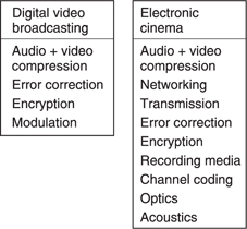
Figure 1.2 Some examples of convergent systems and the technologies in them.
Imaging systems can only be as good as the transducers. Chapter 8 considers displays from the well-established CRT through LCDs up to modern display technologies such as micromirrors, plasma and lasers.
For a given quality, real-time audio and video require a corresponding data rate. Often this rate is not available for economic or practical reasons. This has led to the development of compression techniques such as MPEG which allow the data rate to be reduced. Chapter 9 looks at compression techniques and points out where quality can be lost by the unwary.
Once in the digital domain, audio and images can be manipulated using computer techniques. This can include production and post-production steps such as editing, keying and effects, or practical requirements such as resizing to fit a particular display. Although in principle any digital computer could operate on image data, the data rates needed by some imaging applications are beyond the processing power of a conventional computer and the data rates of its storage systems.
Moving-image processing needs hardware which is optimized for working on large data arrays. The general term for this kind of thing is digital signal processing (DSP). Chapter 2 explains how computers and digital signal processors work.
Data storage is a vital enabling technology and must be treated in some detail. Data can be stored on various media for archiving, rapid retrieval or distribution. The principles and characteristics of magnetic and optical recordings on tape and disks will be found in Chapter 11.
Data can be sent from one place to another in local or wide area networks, on private radio links or public radio broadcasts. Chapter 12 considers all principles of data transmission on copper, optical or radio links.
Whether for storage or transmission, the reliability or integrity of the data is paramount. Data errors cause computer crashes, pops and clicks in the audio and flashes on the screen. The solution is error checking and correction and this is the subject of Chapter 10. Encryption is related strongly to error correction and is important to prevent unauthorized access to sensitive or copyright material. Encryption is also treated in Chapter 10.
1.2 Why binary?
Arithmetically, the binary system is the simplest numbering scheme possible. Figure 1.3(a) shows that there are only two symbols: 1 and 0. Each symbol is a binary digit, abbreviated to bit. One bit is a datum and many bits are data. Logically, binary allows a system of thought in which statements can only be true or false.
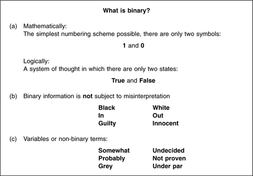
The great advantage of binary systems is that they are the most resistant to misinterpretation. In information terms they are robust. Figure 1.3(b) shows some binary terms and (c) some non-binary terms for comparison. In all real processes, the wanted information is disturbed by noise and distortion, but with only two possibilities to distinguish, binary systems have the greatest resistance to such effects.
Figure 1.4(a) shows an ideal binary electrical signal is simply two different voltages: a high voltage representing a true logic state or a binary 1 and a low voltage representing a false logic state or a binary 0. The ideal waveform is also shown at (b) after it has passed through a real system. The waveform has been considerably altered, but the binary information can be recovered by comparing the voltage with a threshold which is set half-way between the ideal levels. In this way any received voltage which is above the threshold is considered a 1 and any voltage below is considered a 0. This process is called slicing, and can reject significant amounts of unwanted noise added to the signal.
The signal will be carried in a channel with finite bandwidth, and this limits the slew rate of the signal; an ideally upright edge is made to slope. Noise added to a sloping signal (c) can change the time at which the slicer judges that the level passed through the threshold. This effect is also eliminated when the output of the slicer is reclocked. Figure 1.4(d) shows that however many stages the binary signal passes through, the information is unchanged except for a delay.
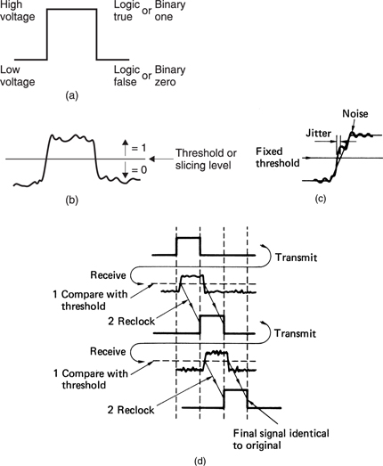
Of course, an excessive noise could cause a problem. If it had sufficient level and the correct sense or polarity, noise could cause the signal to cross the threshold and the output of the slicer would then be incorrect. However, as binary has only two symbols, if it is known that the symbol is incorrect, it need only be set to the other state and a perfect correction has been achieved. Error correction really is as trivial as that, although determining which bit needs to be changed is somewhat more difficult.
Figure 1.5 shows that binary information can be represented by a wide range of real phenomena. All that is needed is the ability to exist in two states. A switch can be open or closed and so represent a single bit. This switch may control the voltage in a wire which allows the bit to be transmitted. In an optical system, light may be transmitted or obstructed. In a mechanical system, the presence or absence of some feature can denote the state of a bit. The presence or absence of a radio carrier can signal a bit. In a random access memory (RAM), the state of an electric charge stores a bit.
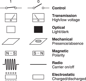
Figure 1.5 also shows that magnetism is naturally binary as two stable directions of magnetization are easily arranged and rearranged as required. This is why digital magnetic recording has been so sucessful: it is a natural way of storing binary signals.
The robustness of binary signals means that bits can be packed more densely onto storage media, increasing the performance or reducing the cost. In radio signalling, lower power can be used.
In decimal systems, the digits in a number (counting from the right, or least significant end) represent ones, tens, hundreds, thousands etc. Figure 1.6(a) shows that in binary, the bits represent one, two, four, eight, sixteen, etc. A multi-digit binary number is commonly called a word, and the number of bits in the word is called the wordlength. The right-hand bit is called the least significant bit (LSB) whereas the bit on the left-hand end of the word is called the most significant bit (MSB). Clearly more digits are required in binary than in decimal, but they are more easily handled. A word of eight bits is called a byte, which is a contraction of ‘by eight'.
Figure 1.6(a) shows some binary numbers and their equivalent in decimal. The radix point has the same significance in binary: symbols to the right of it represent one half, one quarter and so on. Binary is convenient for electronic circuits, which do not get tired, but numbers expressed in binary become very long, and writing them is tedious and error-prone. The octal (b) and hexadecimal (c) notations are both used for writing binary since conversion is so simple. A binary number is split into groups of three or four digits starting at the least significant end, and the groups are individually converted to octal or hexadecimal digits. Since sixteen different symbols are required in hex. the letters A–F are used for the numbers above nine.

The number range is found by raising two to the power of the wordlength. Thus a four-bit word has sixteen combinations, and could address a memory having sixteen locations. A sixteen-bit word has 65 536 combinations. Figure 1.7(a) shows some examples of wordlength and resolution.
Binary words can have a remarkable range of meanings; they may describe the magnitude of a number such as an audio sample, an image pixel or a transform coefficient. Binary words may specify the address of a single location in a memory, or the instruction to be performed by a processor. The capacity of memories and storage media is measured in bytes, but to avoid large numbers, kilobytes, megabytes and gigabytes are often used. A ten-bit word has 1024 combinations, which is close to one thousand. In physics 1k (where the k is lower case) means 1000, whereas in digital terminology, 1K (where the K is upper case) is defined as 1024. However, the wrong case is frequently used. A kilobyte (KB) of memory contains 1024 bytes. A megabyte (1 MB) contains 1024 kilobytes and would need a twenty-bit address. A gigabyte contains 1024 megabytes and would need a thirty-bit address. Figure 1.7(b) shows some examples.

Figure 1.7 The wordlength of a sample controls the resolution as shown in (a). In the same way the ability to address memory locations is also determined as in (b).
1.3 Conversion
Figure 1.8 shows that many different types of information can be expressed as data, or more precisely as binary words. As will be seen, standards have to be agreed for the way in which the range of values the information can take will be mapped onto the available binary number range. Clearly both source and destination must comply with the same standard, otherwise the information will be incorrectly interpreted.
One of the simplest standardized mappings is the American standard code for information interchange (ASCII). Figure 1.9 shows that this is simply a table specifying which binary number is to be used to represent alphanumeric information (letters of the alphabet, numbers and punctuation). As ASCII has limited capability to handle the full richness of the world's tongues, word processors and typesetters have to define more sophisticated mappings to handle the greater range of characters such as italics, subscripts and superscripts and so on.
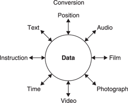
Figure 1.8 A wide variety of information types which can be expressed as binary numbers.

Alphanumeric characters are discrete and it is obvious to allocate one binary word to each character. Where the information is continuous a different approach is necessary. An audio waveform is continuous in one dimension, namely time, whereas a still picture is continuous in two axes, conventionally vertical and horizontal. The shape of a solid object will need to expressed as three-dimensional data for use in CAD (computer aided design) systems and in virtual reality and simulation systems.
The solution here is to use a combination of sampling and interpolation. Sampling is a process of periodic measurement and this can take place in time or space. Interpolation is a filtering process which returns information from discrete points to a continuum. Filtering is inseparable from digital techniques and Chapter 3 treats the subject in some detail.
Sampling can convert the shape of an analog waveform or the surface of a solid into a set of numerically defined points. In image portrayal a grid of defined points is created in the plane of the image and at each one the brightness and colour of the image is measured.
It is vital to appreciate that although the samples carry information about the waveform, they are not themselves the waveform. The waveform can only be observed after the interpolator. Samples should be considered as information-efficient instructions which control an interpolator to re-create a continuum. The failure to interpolate causes distortions and artifacts which may be justified by the need for economy but which are not fundamental to sampling. This topic is important for quality and will be considered in Chapter 4.
Those who are not familiar with digital principles often worry that sampling takes away something from a signal because it is not taking notice of what happened between the samples. This would be true in a system having infinite bandwidth, but no continuous signal can have infinite bandwidth. All signals from transducers have a resolution or frequency response limit, as do human vision and hearing. When a signal has finite bandwidth, the rate at which it can change is limited, and the way in which it changes becomes predictable. If the sampling rate is adequate, a waveform can only change between samples in one way, it is then only necessary to convey the samples and the original waveform can unambiguously be reconstructed from them.

Figure 1.10 In pulse code modulation (PCM), the analog waveform is measured periodically at the sampling rate. The voltage (represented here by the height) of each sample is then described by a whole number. The whole numbers are stored or transmitted rather than the waveform itself.
An audio waveform is sampled in the time domain at a constant sampling frequency Fs as shown in Figure 1.10. In contrast, images are sampled in space. Figure 1.11 shows that a monochrome digital image is a rectangular array of points at which the brightness is stored as a number. The points are known as picture cells, generally abbreviated to pixels, although sometimes the abbreviation is more savage and they are known as pels. As shown in Figure 1.11(a), the array will generally be arranged with an even spacing between pixels, which are in rows and columns. By placing the pixels close together, it is hoped that a combination of the filtering action of the display and the finite resolution of the eye will cause the observer to perceive a continuous image. Obviously the finer the pixel spacing, the greater the resolution of the picture will be, but the amount of data needed to store one picture will increase as the square of the resolution, and with it the costs.
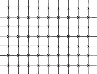
Figure 1.11(a) A picture can be stored digitally by representing the brightness at each of the above points by a binary number. For a colour picture each point becomes a vector and has to describe the brightness, hue and saturation of that part of the picture. Samples are usually but not always formed into regular arrays of rows and columns, and it is most efficient if the horizontal and vertical spacing are the same.
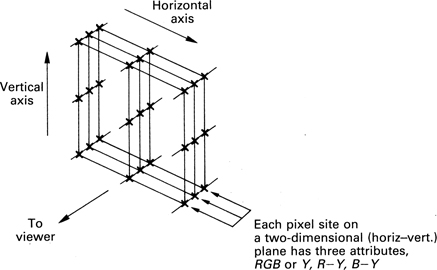
Figure 1.11(b) In the case of component video, each pixel site is described by threevalues and so the pixel becomes a vector quantity
The most efficient system is one in which the horizontal and vertical spacing between pixels is the same. This is because as the viewer approaches the screen, the eye is able to resolve the individual pixels at the same time in both axes. Given a choice, the viewer would then back off until the pixel structure just vanished. Samples taken in this way are called square pixels although this is a misnomer: it is the sampling grid which is square. Computer graphics have always used square pixels, whereas digital television frequently does not.
In displays, colour is created by the additive mixing in the display of three primary colours, typically Red, Green and Blue. Effectively the display needs to be supplied with three video signals, each representing a primary colour. Since practical colour cameras generally also have three seperate sensors, one for each primary colour, a camera and a display can be directly connected. RGB consists of three parallel signals having the same bit rate, and is used where the highest accuracy is needed. RGB is seldom used for broadcast applications because of the high cost.
If RGB is used in the digital domain, it will be seen from Figure 1.11(b) that each image consists of three superimposed layers of samples, one for each primary colour. The pixel is no longer a single number representing a scalar brightness value, but a vector which describes in some way the brightness, hue and saturation of that point in the picture. In RGB, the pixels contain three unipolar numbers representing the proportion of each of the three primary colours at that point in the picture.
In colour printing, subtractive mixing is used, which is quite different from the additive mixing of television. In subtractive mixing, the primaries are cyan, magenta and yellow. If all these are used together, the result is black, but it is easier to use black pigments for this purpose and so colour printing uses four channels, cyan, magenta, yellow and black or CMYK. It is possible to convert from RGB to CYMK so that images captured by video cameras or digital still cameras can be reproduced as prints. Chapter 6 deals with colour conversion.
Samples are taken at instants in time or space and the value of each one is then mapped onto a range of binary numbers by a process called quantizing. The range is determined by the wordlength. As the wordlength is an integer, the binary number ranges available always differ by a factor of two.
In video signals, which are non-linear, eight-bit words allowing 256 combinations are adequate. Linear light coding requires as much as fourteen-bit resolution. In a Compact Disc, the numbers have sixteen bits and 65 536 different codes are available. For audio production purposes longer wordlengths are needed. Audio information is bipolar and is handled by the two's complement coding scheme discussed in section 2.4.
Perfect quantizing causes artifacts in both audio and video and a technique known as dither is essential to overcome the problem. Quantizing and dither techniques are discussed in Chapter 4.
There are two ways in which binary signals can be used to carry sample data and these are shown in Figure 1.12. When each digit of the binary number is carried on a separate wire this is called parallel transmission. The state of the wires changes at the sampling rate. Using multiple wires is cumbersome, and a single conductor or fibre can be used where successive digits from each sample are sent serially. This is the definition of pulse code modulation which was patented by Reeves.1 Clearly the clock frequency must now be higher than the sampling rate.

A single high-quality PCM audio channel requires around one million bits per second. Digital audio came into wide use as soon as such a data rate could be handled economically. A PCM standard definition moving colour picture requires around 200 million bits per second. Clearly digital video production could only become common some time after digital audio. Consumer digital video applications could only become possible when technology became available to reduce or compress the data rate.
Whichever type of information in Figure 1.8 is used, the result is always the same: binary numbers. As all binary numbers look the same, it is impossible to tell whether a set of such numbers contains images, audio or text without some additional information. File name extensions are one approach to this. In general, binary data only become meaningful information when they arrive at a destination which adheres to the same mapping as the encoder, or at a DSP device which is programmed to understand that mapping so that it can manipulate the data. Storage and transmission systems in general couldn't care less what the data mean. All they have to do is deliver it accurately and it becomes the problem of the destination to figure out what it means. This is a tremendous advantage because it means that storage and transmission systems are generic and largely independent of the type of data.
In practice the only significant differences between types of data that concern transmission and storage devices are the tolerance of the data to error and the degree to which real time needs to be approached at the destination.
1.4 Integrated circuits
Integrated circuits are electronic systems where all the components have been shrunk to fit in a single part. They are also commonly called chips although strictly this refers to the actual circuit element inside the protective housing. The advantage of integrated circuits is that the unit cost can be very low. The development and tooling cost, however, is considerable, so integrated circuits are only economically viable if they are made in volume. Consumer products are an ideal market.
The smaller each component can be, and the closer they can be packed, the more functionality can be obtained from the part, without any increase in cost. Inside such circuits, the small spacing between the wires results in crosstalk where signals in one wire are picked up by others. Binary systems resist crosstalk and allow denser packing than would be possible with linear or analog circuits. As a result, binary logic and integrated circuits form a natural alliance. The integrated circuit has been the subject of phenomenal progress in packing density which continues to drive costs down.
When it became possible to put all the functionality of a central processing unit (CPU) on a single integrated circuit, the result was the microprocessor. Computing power came within the reach of the consumer and led to the explosion in personal computers.
The functionality of integrated circuits goes up with time with the following results:
(a)Existing processes become cheaper: e.g the price of pocket calculators.
(b)Processes which were previously too complex become affordable; e.g. error correction and compression.
(c)The cost of RAM falls.
As a result, devices based on complex processes become available not when they are invented but when the economics of integrated circuits make them feasible. A good example is the Compact Disc. The optical storage technology of CD is much older, but it became possible to use it as a consumer digital audio product when real-time error-correction processors became available at consumer prices. Similarly, digital television was not viable until compression processors, which are more complex still, became economic.
1.5 Storage technology
Advances in integrated circuits do not just improve the performance of RAM and computers. Integrated circuits are used in storage devices such as disk drives to encode and correct the data as well as to control the mechanism and make the heads follow the data tracks. If more complex coding and control can be used, the storage density can rise. In parallel with this, the performance of heads and media continues to improve and when compounded with the coding and control improvements, each generation of storage device displays a significant reduction in the cost of storing a given quantity of data. This makes new applications possible which were previously too expensive. For example, the falling cost of the hard disk drive led first to the word processor in the 1970s, which needs a relatively small amount of data, next to the digital audio editor in the 1980s and then to the video editor in the 1990s.
Storage devices are generally classified by their access time and the cost per bit. Unfortunately these two parameters are mutually exclusive and improving one usually worsens the other. Figure 1.13 shows the relative merits of RAM, disks and tape. RAM has the fastest access, but is extremely expensive because every bit has to be individually fabricated inside the integrated circuit. Magnetic recording is cheaper because the medium is uniform and the bits are created by the passage of the head. Disks are optimized for speed whereas tapes are optimized for capacity. As a result, various different storage technologies co-exist because no single one has all the ideal features. The performance of all storage technologies increases with time, but the relative performance tends to stay the same.
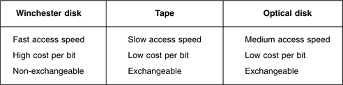
Figure 1.13 Different storage media have different combinations of attributes and no one technology is superior in all aspects.
Optical disks such as CD/CDROM and DVD are optimized for mass replication by pressing and cannot be recorded. Recordable optical disks such as CD-R and DVD-R are also available and these have the advantage of high capacity and exchangeability but usually fall behind magnetic disks in access time and transfer rate.
1.6 Noise and probability
Probability is a useful concept when dealing with processes which are not completely predictable. Thermal noise in electronic components is random, and although under given conditions the noise power in a system may be constant, this value only determines the heat that would be developed in a resistive load. In digital systems, it is the instantaneous voltage of noise which is of interest, since it is a form of interference which could alter the state of a bit if it were large enough. Unfortunately the instantaneous voltage cannot be predicted; indeed if it could the interference could not be called noise. Noise can only be quantified statistically, by measuring or predicting the likelihood of a given noise amplitude.
Figure 1.14 shows a graph relating the probability of occurrence to the amplitude of noise. The noise amplitude increases away from the origin along the horizontal axis, and for any amplitude of interest, the probability of that noise amplitude occurring can be read from the curve. The shape of the curve is known as a Gaussian distribution, which crops up whenever the overall effect of a large number of independent phenomena is considered. Thermal noise is due to the contributions from countless molecules in the component concerned. Magnetic recording depends on superimposing some average magnetism on vast numbers of magnetic particles.

Figure 1.14 The endless nature of the Gaussian curve means that errors will always happen and a correction scheme is usually necessary.
If it were possible to isolate an individual noise-generating microcosm of a tape or a head on the molecular scale, the noise it could generate would have physical limits because of the finite energy present. The noise distribution might then be rectangular as shown in Figure 1.15(a), where all amplitudes below the physical limit are equally likely. The output of a random number generator can have a uniform probability if each possible value occurs once per sequence.
If the combined effect of two of these uniform probability processes is considered, clearly the maximum amplitude is now doubled, because the two effects can add, but provided the two effects are uncorrelated, they can also subtract, so the probability is no longer rectangular, but becomes triangular as in Figure 1.15(b). The probability falls to zero at peak amplitude because the chances of two independent mechanisms reaching their peak value with the same polarity at the same time are understandably small.
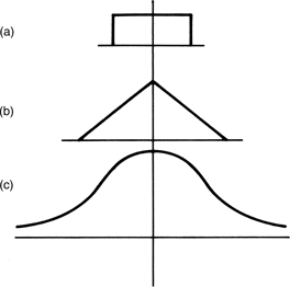
Figure 1.15 At (a) is a rectangular probability; all values are equally likely but between physical limits. At (b) is the sum of two rectangular probabilities, which is triangular, and at (c) is the Gaussian curve which is the sum of an infinite number of rectangular probabilities.
If the number of mechanisms summed together is now allowed to increase without limit, the result is the Gaussian curve shown in Figure 1.15(c), where it will be seen that the curve has no amplitude limit, because it is just possible that all mechanisms will simultaneously reach their peak value together, although the chances of this happening are incredibly remote. Thus the Gaussian curve is the overall probability of a large number of uncorrelated uniform processes.
Many people have difficulty dealing with probability or statistical information. A motorcyclist once told me he would not fly in a helicopter because they are unsafe. When told that smoking increases the probability of lung cancer, many people will cite some 80-year-old relative who has smoked every day for 60 years and is still fit. This is not at odds with statistics at all. The Gaussian curve is infinite and permits, indeed requires, a small number of surviving heavy smokers.
There two wonderful examples of extremes of probability. At the high probability end are the chances of a celluloid cat being chased through hell by an asbestos dog, for which gem I am indebted to Robert Pease. At the low probability end is a quote from a competition held by New Scientist for newspaper headlines which would amuse scientists: National Lottery winner struck by lightning!
1.7 Time compression and expansion
Data files such as computer programs are simply lists of instructions and have no natural time axis. In contrast, audio and video data are sampled at a fixed rate and need to be presented to the viewer at the same rate. In audiovisual systems the audio also needs to be synchronized to the video. Continuous bitstreams at a fixed bit rate are difficult for generic data recording and transmission systems to handle. Most digital storage and network systems work on blocks of data which be individually addressed and/or routed. The bit rate may be fixed at the design stage at a value which may be too low or too high for the audio or video data to be handled.
The solution is to use time compression or expansion. Figure 1.16 shows a RAM which is addressed by binary counters which periodically overflow to zero and start counting again, giving the RAM a ring structure. If write and read addresses increment at the same speed, the RAM becomes a fixed data delay as the addresses retain a fixed relationship. However, if the read address clock runs at a higher frequency, but in bursts, the output data are assembled into blocks with spaces in between. The data are now time compressed. Instead of being an unbroken stream which is difficult to handle, the data are in blocks with convenient pauses in between them. In these pauses numerous processes can take place. A hard disk might move its heads to another track. In all types of recording and transmission, the time compression of the samples allows time for synchronizing patterns, subcode and errorcorrection words to be inserted.
Subsequently, any time compression can be reversed by time expansion. This requires a second RAM identical to the one shown. Data are written into the RAM in bursts, but read out at the standard sampling rate to restore a continuous bitstream. In a recorder, the time expansion stage can be combined with the timebase correction stage so that speed variations in the medium can be eliminated at the same time. The use of time compression is universal in digital recording and widely used in transmission. In general, the instantaneous data rate in the channel is not the same as the original rate although in real-time systems the average rate must be the same.

Figure 1.16 If the memory address is arranged to come from a counter which overflows, the memory can be made to appear circular. The write address then rotates endlessly, overwriting previous data once per revolution. The read address can follow the write address by a variable distance (not exceeding one revolution) and so a variable delay takes place between reading and writing.

Where the bit rate of the communication path is inadequate, transmission is still possible, but not in real time. Figure 1.17 shows that the data to be transmitted will have to be written in real time on a storage device such as a disk drive, and the drive will then transfer the data at whatever rate is possible to another drive at the receiver. When the transmission is complete, the second drive can then provide the data at the correct bit rate.
In the case where the available bit rate is higher than the correct data rate, the same configuration can be used to copy an audio or video data file faster than real time. Another application of time compression is to allow several streams of data to be carried along the same channel in a technique known as multiplexing. Figure 1.18 shows some examples. At (a) multiplexing allows audio and video data to be recorded on the same heads in a digital video recorder such as DVC. At (b), several TV channels are multiplexed into one MPEG transport stream.
1.8 Error correction and concealment
All practical recording and transmission media are imperfect. Magnetic media, for example, suffer from noise and dropouts. In a digital recording of binary data, a bit is either correct or wrong, with no intermediate stage. Small amounts of noise are rejected, but inevitably, infrequent noise impulses cause some individual bits to be in error. Dropouts cause a larger number of bits in one place to be in error. An error of this kind is called a burst error. Whatever the medium and whatever the nature of the mechanism responsible, data are either recovered correctly or suffer some combination of bit errors and burst errors. In optical disks, random errors can be caused by imperfections in the moulding process, whereas burst errors are due to contamination or scratching of the disk surface.


Figure 1.18(b) In MPEG, multiplexing allows data from several TV channels to share one bitstream.
Before attempting to specify an error-correction system, the causes of errors must be studied to quantify the problem, and the sensitivity of the destination to errors must be assessed. In video and audio the sensitivity to errors must be subjective. Figure 1.19 shows the relative sensitivity of different types of data to error.
Whilst the exact BER (bit error rate) which can be tolerated will depend on the application, digital audio is less tolerant of errors than digital video and more tolerant than computer data. The use of compression changes the picture if redundancy has been removed from a signal, it becomes less tolerant of errors.
In PCM audio and video, the effect of a single bit in error depends upon the significance of the bit. If the least significant bit of a sample is wrong, the chances are that the effect will be lost in the noise. Conversely, if a high-order bit is in error, a massive transient will be added to the waveform.

MPEG video compression uses variable-length coding. If a bit error occurs it may cause the length of a symbol to be incorrectly assessed and the decoder will lose synchronism with the bitstream. This may cause an error affecting a significant area of the picture which might propagate from one picture to the next.
If the maximum error rate which the destination can tolerate is likely to be exceeded by the unaided channel, some form of error handling will be necessary.
There are a number of terms which have idiomatic meanings in error correction. The raw BER is the error rate of the medium, whereas the residual or uncorrected BER is the rate at which the error-correction system fails to detect or miscorrects errors. In practical digital systems, the residual BER is negligibly small. If the error correction is turned off, the two figures become the same.
It is paramount in all error-correction systems that the protection used should be appropriate for the probability of errors to be encountered. An inadequate error-correction system is actually worse than not having any correction. Error correction works by trading probabilities. Error-free performance with a certain error rate is achieved at the expense of performance at higher error rates. Figure 1.20 shows the effect of an errorcorrection system on the residual BER for a given raw BER. It will be seen that there is a characteristic knee in the graph. If the expected raw BER has been misjudged, the consequences can be disastrous. Another result demonstrated by the example is that we can only guarantee to detect the same number of bits in error as there are redundant bits.
There are many different types of recording and transmission channel and consequently there will be many different mechanisms which may result in errors. Although there are many different applications, the basic principles remain the same.

In magnetic recording, data can be corrupted by mechanical problems such as media dropout and poor tracking or head contact, or Gaussian thermal noise in replay circuits and heads. In optical recording, contamination of the medium interrupts the light beam. Warped disks and birefringent pressings cause defocusing. Inside equipment, data are conveyed on short wires and the noise environment is under the designer's control. With suitable design techniques, errors can be made effectively negligible. In communication systems, there is considerably less control of the electromagnetic environment.
In cables, crosstalk and electromagnetic interference occur and can corrupt data, although optical fibres are resistant to interference of this kind. In long-distance cable transmission the effects of lightning and exchange switching noise must be considered. In digital television broadcasting, multipath reception causes notches in the received spectrum where signal cancellation takes place. In MOS memories the datum is stored in a tiny charge well which acts as a capacitor (see Chapter 2) and natural radioactive decay can cause alpha particles which have enough energy to discharge a well, resulting in a single bit error. This only happens once every few decades in a single chip, but when large numbers of chips are assembled in computer memories the probability of error rises to one every few minutes.
Irrespective of the cause, error mechanisms cause one of two effects. There are large isolated corruptions, called error bursts, where numerous bits are corrupted all together in an area which is otherwise error free, and there are random errors affecting single bits or symbols. Whatever the mechanism, the result will be that the received data will not be exactly the same as those sent. It is a tremendous advantage of digital systems that the discrete data bits will be each either right or wrong. A bit cannot be off-colour as it can only be interpreted as 0 or 1. Thus the subtle degradations of analog systems are absent from digital recording and transmission channels and will only be found in convertors. Equally if a binary digit is known to be wrong, it is only necessary to invert its state and then it must be right and indistinguishable from its original value!
Some conclusions can be drawn from the Gaussian distribution of noise.2 First, it is not possible to make error-free digital recordings, because however high the signal-to-noise ratio of the recording, there is still a small but finite chance that the noise can exceed the signal. Measuring the signal-to-noise ratio of a channel establishes the noise power, which determines the width of the noise distribution curve relative to the signal amplitude.
When in a binary system the noise amplitude exceeds the signal amplitude, but with the opposite polarity, a bit error will occur. Knowledge of the shape of the Gaussian curve allows the conversion of signal-to-noise ratio into bit error rate (BER). It can be predicted how many bits will fail due to noise in a given recording, but it is not possible to say which bits will be affected. Increasing the SNR of the channel will not eliminate errors, it just reduces their probability. The logical solution is to incorporate an error-correction system.
Figure 1.21 shows that error correction works by adding some bits to the data which are calculated from the data. This creates an entity called a codeword which spans a greater length of time than one bit alone. The statistics of noise mean that whilst one bit may be lost in a codeword, the loss of the rest of the codeword because of noise is highly improbable. As will be described later in this chapter, codewords are designed to be able totally to correct a finite number of corrupted bits. The greater the timespan over which the coding is performed, or, on a recording medium, the greater area over which the coding is performed, the greater will be the reliability achieved, although this does mean a greater encoding and decoding delay.

Figure 1.21 Error correction works by adding redundancy
Shannon3 disclosed that a message can be sent to any desired degree of accuracy provided that it is spread over a sufficient timespan. Engineers have to compromise, because an infinite coding delay in the recovery of an error-free signal is not acceptable. Most short digital interfaces do not employ error correction because the build-up of coding delays in production systems is unacceptable.
If error correction is necessary as a practical matter, it is then only a small step to put it to maximum use. All error correction depends on adding bits to the original message, and this, of course, increases the number of bits to be recorded, although it does not increase the information recorded. It might be imagined that error correction is going to reduce storage capacity, because space has to be found for all the extra bits. Nothing could be further from the truth. Once an error-correction system is used, the signal-to-noise ratio of the channel can be reduced, because the raised BER of the channel will be overcome by the errorcorrection system.
In a digital television broadcast system the use of error correction allows a lower-powered transmitter to be used. In a magnetic track, reduction of the SNR by 3 dB can be achieved by halving the track width, provided that the system is not dominated by head or preamplifier noise. This doubles the recording density, making the storage of the additional bits needed for error correction a trivial matter. In short, error correction is not a nuisance to be tolerated; it is a vital tool needed to maximize the efficiency of systems. Convergent technologies would not be economically viable without it.
Figure 1.22 shows the broad approaches to data integrity. The first stage might be called error avoidance and includes such measures as creating bad block files on hard disks or using verified media. The data pass through the channel, where corruption may occur. On receipt of the data the occurrence of errors is first detected, and this process must be extremely reliable, as it does not matter how effective the correction or how good the concealment algorithm, if it is not known that they are necessary! The detection of an error then results in a course of action being decided.

Figure 1.22 Approaches to errors. See text for details.
In many cases of digital video or audio replay a retry is not possible because the data are required in real time. However, if a disk-based system is transferring to tape for the purpose of backup, real-time operation is not required. If the disk drive detects an error a retry is easy as the disk is turning at several thousand rpm and will quickly re-present the data. An error due to a dust particle may not occur on the next revolution. Many magnetic tape systems have read after write. During recording, offtape data are immediately checked for errors. If an error is detected, the tape will abort the recording, reverse to the beginning of the current block and erase it. The data from that block are then recorded further down the tape. This is the recording equivalent of a retransmission in a communications system.
In binary, a bit has only two states. If it is wrong, it is only necessary to reverse the state and it must be right. Thus the correction process is trivial and perfect. The main difficulty is in identifying the bits which are in error. This is done by coding the data by adding redundant bits. Adding redundancy is not confined to digital technology, airliners have several engines and cars have twin braking systems. Clearly the more failures which have to be handled, the more redundancy is needed. If a fourengined airliner is designed to fly normally with one engine failed, three of the engines have enough power to reach cruise speed, and the fourth one is redundant. The amount of redundancy is equal to the amount of failure which can be handled. In the case of the failure of two engines, the plane can still fly, but it must slow down; this is graceful degradation. Clearly the chances of a two-engine failure on the same flight are remote.
The amount of error which can be corrected is proportional to the amount of redundancy, and it will be shown in Chapter 10 that within this limit, the data are returned to exactly their original value. Consequently corrected samples are undetectable. If the amount of error exceeds the amount of redundancy, correction is not possible, and, in order to allow graceful degradation, concealment will be used. Concealment is a process where the value of a missing sample is estimated from those nearby. The estimated sample value is not necessarily exactly the same as the original, and so under some circumstances concealment can be audible, especially if it is frequent. However, in a well-designed system, concealments occur with negligible frequency unless there is an actual fault or problem.
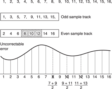
Figure 1.23 In cases where the error correction is inadequate, concealment can be used provided that the samples have been ordered appropriately in the recording. Odd and even samples are recorded in different places as shown here. As a result an uncorrectable error causes incorrect samples to occur singly, between correct samples. In the example shown, sample 8 is incorrect, but samples 7 and 9 are unaffected and an approximation to the value of sample 8 can be had by taking the average value of the two. This interpolated value is substituted for the incorrect value.
Concealment is made possible by rearranging the sample sequence prior to recording. This is shown in Figure 1.23 where odd-numbered samples are separated from even-numbered samples prior to recording. The odd and even sets of samples may be recorded in different places on the medium, so that an uncorrectable burst error affects only one set. On replay, the samples are recombined into their natural sequence, and the error is now split up so that it results in every other sample being lost in a two-dimensional structure. The picture is now described half as often, but can still be reproduced with some loss of accuracy. This is better than not being reproduced at all even if it is not perfect. Many digital video recorders use such an odd/even distribution for concealment. Clearly if any errors are fully correctable, the distribution is a waste of time; it is only needed if correction is not possible.
The presence of an error-correction system means that the video (and audio) quality is independent of the medium/head quality within limits. There is no point in trying to assess the health of a machine by watching a monitor or listening to the audio, as this will not reveal whether the error rate is normal or within a whisker of failure. The only useful procedure is to monitor the frequency with which errors are being corrected, and to compare it with normal figures.

Figure 1.24(a) Interleaving is essential to make error-correction schemes more efficient. Samples written sequentially in rows into a memory have redundancy P added to each row. The memory is then read in columns and the data sent to the recording medium. On replay the non-sequential samples from the medium are de-interleaved to return them to their normal sequence. This breaks up the burst error (shaded) into one error symbol per row in the memory, which can be corrected by the redundancy P.

Figure 1.24(b) In addition to the redundancy P on rows, inner redundancy Q is also generated on columns. On replay, the Q code checker will pass on flag F if it finds an error too large to handle itself. The flags pass through the de-interleave process and are used by the outer error correction to identify which symbol in the row needs correcting with P redundancy. The concept of crossing two codes in this way is called a product code.
Digital systems such as broadcasting, optical disks and magnetic recorders are prone to burst errors. Adding redundancy equal to the size of expected bursts to every code is inefficient. Figure 1.24(a) shows that the efficiency of the system can be raised using interleaving. Sequential samples from the ADC are assembled into codes, but these are not recorded/transmitted in their natural sequence. A number of sequential codes are assembled along rows in a memory. When the memory is full, it is copied to the medium by reading down columns. Subsequently, the samples need to be de-interleaved to return them to their natural sequence. This is done by writing samples from tape into a memory in columns, and when it is full, the memory is read in rows. Samples read from the memory are now in their original sequence so there is no effect on the information. However, if a burst error occurs as is shown shaded in the figure it will damage sequential samples in a vertical direction in the de-interleave memory. When the memory is read, a single large error is broken down into a number of small errors whose size is exactly equal to the correcting power of the codes and the correction is performed with maximum efficiency.
An extension of the process of interleave is where the memory array has not only rows made into codewords, but also columns made into codewords by the addition of vertical redundancy. This is known as a product code. Figure 1.24(b) shows that in a product code the redundancy calculated first and checked last is called the outer code, and the redundancy calculated second and checked first is called the inner code. The inner code is formed along tracks on the medium. Random errors due to noise are corrected by the inner code and do not impair the burstcorrecting power of the outer code. Burst errors are declared uncorrectable by the inner code which flags the bad samples on the way into the de-interleave memory. The outer code reads the error flags in order to locate the erroneous data. As it does not have to compute the error locations, the outer code can correct more errors.
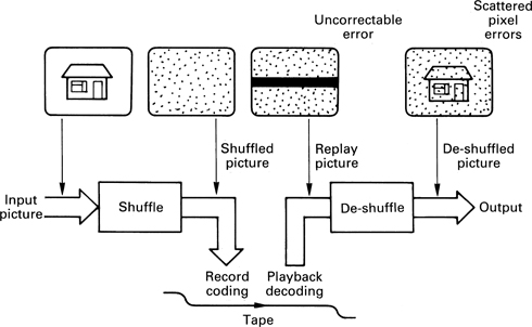
Figure 1.25 The shuffle before recording and the corresponding de-shuffle after playback cancel out as far as the picture is concerned. However, a block of errors due to dropout only experiences the de-shuffle, which spreads the error randomly over the screen. The pixel errors are then easier to correct.
The interleave, de-interleave, time-compression and timebase-correction processes inevitably cause delay.
When a product code-based recording suffers an uncorrectable error in an image such as a TV picture or a computer graphic, the result is a rectangular block of failed sample values which require concealment. Such a regular structure would be visible even after concealment, and an additional process is necessary to reduce the visibility. Figure 1.25 shows that a shuffle process is performed prior to product coding in which the pixels are moved around the picture in a pseudo-random fashion. The reverse process is used on replay, and the overall effect is nullified. However, if an uncorrectable error occurs, this will only pass through the de-shuffle and so the regular structure of the failed data blocks will be randomized. The errors are spread across the picture as individual failed pixels in an irregular structure.
1.9 Channel coding
In most recorders used for storing data, the medium carries a track which reproduces a single waveform. Clearly data words contain many bits and so they have to be recorded serially, a bit at a time. Some media, such as optical or magnetic disks, have only one active track, so they must be totally self-contained. DVTRs may have one, two or four tracks read or written simultaneously. At high recording densities, physical tolerances cause phase shifts, or timing errors, between tracks and so it is not possible to read them in parallel. Each track must still be self-contained until the replayed signal has been timebase corrected.
Recording data serially is not as simple as connecting the serial output of a shift register to the head. Data words may contain strings of identical bits. If a shift register is loaded with such a sample and shifted out serially, the output stays at a constant level for the period of the identical bits, and no event is recorded on the track. On replay there is nothing to indicate how many bits were present, or even how fast to move the medium. Clearly, serialized raw data cannot be recorded directly, it has to be modulated into a waveform which contains an embedded clock irrespective of the values of the bits in the samples. On replay a circuit called a data separator can lock to the embedded clock and use it to separate strings of identical bits.
The process of modulating serial data to make it self-clocking is called channel coding. Channel coding also shapes the spectrum of the serialized waveform to make it more efficient. With a good channel code, more data can be stored on a given medium. Spectrum shaping is used in optical disks to prevent the data from interfering with the focus and tracking servos, and in hard disks and in certain tape formats to allow rerecording without erase heads.
Channel coding is also needed to broadcast digital television signals where shaping of the spectrum is an obvious requirement to avoid interference with other services. The techniques of channel coding for recording and transmission are described in Chapter 10.
1.10 Compression, JPEG and MPEG
In its native form, PCM audio and images may have a data rate which is too high for the available channel. One approach to the problem is to use compression which reduces that rate significantly with a moderate loss of subjective quality. The human eye is not equally sensitive to all spatial frequencies and in the same way the ear is not equally sensitive to all temporal frquencies. Some coding gain can be obtained by using fewer bits to describe the frequencies which are less well perceived. Images typically contain a great deal of redundancy where flat areas contain the same pixel value repeated many times. In moving images there is little difference between one picture and the next, and compression can be achieved by sending only the differences.
The ISO has established compression standards for audio, still and moving images. The still image coding was standardized by the Joint Photographic Experts Group (JPEG), whereas the moving image and audio coding was standardized by the Moving Picture Experts Group (MPEG).
Whilst these techniques may achieve considerable reduction in bit rate, it must be appreciated that lossy compression systems reintroduce the generation loss of the analog domain to digital systems. As a result high compression factors are only suitable for final delivery of fully produced material to the viewer.
For production purposes, compression may be restricted to exploiting the redundancy within each picture individually and then with a mild compression factor. This allows simple algorithms to be used and also permits multiple-generation work without artifacts being visible. Such an approach is used in disk-based workstations.
A consumer product may need only single-generation operation and has simple editing requirements. A much greater degree of compression can then be used, which takes advantage of redundancy between pictures. The same is true for broadcasting, where bandwidth is at a premium. A similar approach may be used in disk-based camcorders which are intended for ENG purposes.
The future of television broadcasting (and of any high-definition television) lies completely in compression technology. Compression requires an encoder prior to the medium and a compatible decoder after it. Extensive consumer use of compression could not occur without suitable standards. The ISO–MPEG coding standards were specifically designed to allow wide interchange of compressed video and audio data. Digital television broadcasting and DVD both use MPEG standard bitstreams and these are detailed in Chapter 9.
Figure 1.26 shows that the output of a single compressor is called an elementary stream. In practice audio and video streams of this type can be combined using multiplexing. The program stream is optimized for recording and the multiplexing is based on blocks of arbitrary size. The transport stream is optimized for transmission and is based on blocks of constant size.
In production equipment such as workstations and VTRs which are designed for editing, the MPEG standard is less useful and many successful products use non-MPEG compression.
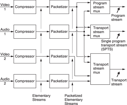
Figure 1.26 The bitstream types of MPEG-2. See text for details.
Compression and the corresponding decoding are complex processes and take time, adding to existing delays in signal paths. Concealment of uncorrectable errors is also more difficult on compressed data. Many compression techniques are based on transforms which are treated in Chapter 3.
1.11 Convergence and commercial television
When television had little or no competition, it could pretty much do what it liked, but now there are alternatives. As a carrier of information, commercial television doesn't work very well because its business model is based on the assumption that commercials and programs are inseparable. Aesthetically speaking, advertising and entertainment do not sit well together and the business model is a crude one which evolved when technology was equally crude.
Today convergent technology allows advertising and entertainment to be separated calling into question the business model of commercial television.
The prospective purchaser looking for product or service is alert and has in the author's mind the constraints and desired qualities needed to solve a real-world problem with some time pressure. In contrast when the same person wants to relax and be entertained the real world and its pressures are not wanted. As commercial television tries to serve both requirements at once it must fail. If it sets out to entertain, the artistic thread of any worthwhile drama is irrepairably damaged by commercial breaks. On the other hand, if it sets out to advertise, it does so very inefficiently. Conventional television advertising is like carpet bombing. The commercial is shown to everybody, whether they are interested or not.
The biggest vulnerability of commercial television is that it is linear. Everything comes out in a predetermined sequence which was at one time out of the viewer's control. It is useful to compare television with magazines. These contain articles, which correspond to programs, and advertising. However, there is no compulsion to read all the advertisements in a magazine at a particular time or at all. This makes a magazine a non-linear or random-access medium.
The development of the consumer VCR was a small step to end the linearity of commercial television. Increasing numbers of viewers use VCRs not just as time shifters but also as a means of fast-forwarding through the commercial breaks.
The non-linear storage of video was until recently restricted by economics to professional applications. However, with the falling cost of hard drives, non-linear video storage is now a consumer product.
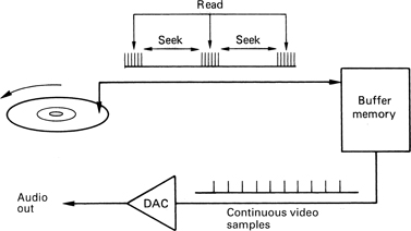
Figure 1.27 In a hard disk recorder, a large-capacity memory is used as a buffer or timebase corrector between the convertors and the disk. The memory allows the convertors to run constantly despite the interruptions in disk transfer caused by the head moving between tracks.
The operation of a hard drive is explained in Chapter 11. What matters here is what it can do. Unlike tape, which can only record or play back but not both at the same time, a PVR can do both simultaneously at arbitrary points on a time line. Figure 1.27 shows how it is done. The disk drive can transfer data much faster than the required bit rate, and so it transfers data in bursts which are smoothed out by RAM buffers. The disk simply interleaves read and write functions so that it gives the impression of reading and writing simultaneously. The read and write processes can take place from anywhere on the disk.
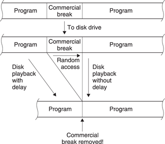
Clearly the PVR can be used as an ordinary video recorder, but it can do some other tricks. Figure 1.28 shows the most far-reaching trick. The disk drive starts recording an off-air commercial TV station. A few minutes later the viewer starts playing back the recording. When the commercial break is transmitted, the disk drive may record it, but the viewer can skip over it using the random access of the hard drive. With suitable software the hard drive could skip over the commercial break automatically by simply not recording it.
When used with digital television systems, the PVR can simply record the transmitted transport stream data and replay it into an MPEG decoder. In this way the PVR has no quality loss whatsoever. The picture quality will be the same as off-air.
Whilst the PVR threatens commercial TV as it is being watched, other technologies threaten to reduce the amount of off-air viewing. The growth of personal computers and the Internet means that there is now an alternative way for the individual to locate products. The would-be purchaser can find a web site which offers the kind of product he or she is looking for, and browse through a virtual catalogue. By clicking on an item of interest, it can, for example, be portrayed in action in a moving video sequence. If it suits, it can be bought there and then.
The Internet allows moving pictures to be delivered to the home without using radio technology. Surely radio technology is only necessary when equipment needs to be genuinely mobile. When a television set is permanently chained to the wall by the power cord, why are we using radio to communicate with it? Most PCs are now capable of playing DVDs, which further erodes off-air viewing.
1.12 Electronic cinema
The traditional film-based cinema has hardly changed in principle for about a century. One of the greatest difficulties is the release of a popular new movie. In order to open simultaneously in a large number of cinemas, an equally large number of prints are needed. As film is based on silver, these prints are expensive. The traditional solution was to divide the world up into regions and rely on poor communications so that new films could be released in each region at a time.
When the digital video disk (DVD) was developed, although it is not expensive to duplicate, Hollywood attempted to impose area codes on the disks so they would not play in another region's players. The idea was that DVDs would not be available until after the cinema release.
The region code of DVDs is exactly the wrong solution. Instead of preventing the reasonable use of a successful modern technology because it reveals the shortcomings of an older technology, the correct solution must be to improve the older technology.
Digital technology allows an arbitrary number of copies of moving image data to be delivered anywhere on earth, and so in principle every electronic cinema on the planet could screen the same movie, ending forever the problem of release prints. Digital technology also eliminates film scratches and dirt, and encryption prevents piracy.
References
1. Reeves, A.H., US Patent 2,272,070
2. Michaels, S.R., Is it Gaussian? Electronics World and Wireless World, 72–73 (Jan. 1993)
3. Shannon, C.E., A mathematical theory of communication. Bell System Tech. J., 27, 379 (1948)