
5
Sound
5.1 Introduction
Sound is important in convergent systems both in its own right and as an accompaniment to some form of image. Traditionally the consumer could receive sound radio at a time decided by the broadcaster, or purchase prerecorded media. Digital technology allows a much greater variety of sound-delivery mechanisms. Sound radio is now broadcast digitally, with greater resistance to multipath reception than analog FM could offer, but still at a time decided by the broadcaster. Prerecorded media reached their pinnacle of sound quality with the Compact Disc, followed by the smaller but audibly inferior MiniDisc, but these are only digitized versions of earlier services.
However, network technology allows digital audio to be delivered to any desired quality and at any time. Figure 5.1 shows one service which is already established. The service provider maintains file servers which contain music in a compressed digital format (typically MPEG Layer III also known as MP3). The consumer can download these files to a PC over the Internet, and can then transfer the files to a RAM-based portable player which contains an MPEG decoder. The sound quality is not outstanding, but the service has the advantage of immediacy and flexibility. The consumer can access audio files from anywhere and create a personalized album in a RAM player.
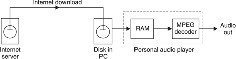
Figure 5.1 Using heavy compression, digital audio recordings can be transferred over the Internet to a PC and thence to a RAM-based player in non-real-time. The compression decoder in the player accesses the RAM to produce real-time audio.
At greater cost, audio data can be exchanged between recording studios using mild or no compression, giving a faster alternative to the delivery of tapes. Clearly a range of sound qualities will be required according to the service, ranging from voice-grade message services to downloadable classical music. This chapter takes the approach that if it shows how to make the finest possible sound reproduction system, the reader can always take an economic decision to provide lower quality. Consequently the information provided here represents as far as possible the state of the art.
Digital multiplexing makes it easy to deliver surround sound and this adds greater involvement to certain moving-image material both in the home and in electronic cinemas. It has been shown beyond doubt that realistic sound causes the viewer to rate the subjective picture quality higher. This is true not only of electronic cinema but also for Internet video where the picture quality is frequently mediocre due to bit rate limitations.
The electronic cinema has the advantage over the home theatre that a greater sum can be invested in the sound equipment, although a small proportion of home theatre systems will also be highly specified. The flat display screen using plasma technology is often hailed as the ultimate TV set to hang on the wall, but a moment’s thought will reveal that without flat loudspeaker technology of high quality, the flat screen is not a TV, but only a display. Most of today’s flat screens contain loudspeakers which are truly appalling and inconsistent with the current high cost of such displays.
It should not be assumed that audio is used entirely for entertainment. Some audio applications, such as aircaft noise monitoring, submarine detection and battlefield simulators, result in specifications which are extremely high. Emergency evacuation instructions in public places come from audio systems which must continue to work in the presence of cable damage, combustion products, water and power loss.
By definition, the sound quality of an audio system can only be assessed by the human auditory system (HAS). Quality means different things to different people and can range from a realistic reproduction of classical music to the intelligible delivery of speech in a difficult acoustic. Many items of audio equipment can only be designed well with a good knowledge of the human hearing mechanism. The understanding of the HAS and how it relates to the criteria for accurate sound reproduction has increased enormously in recent years and these findings will be given here. From this knowledge it becomes obvious what will and will not work and it becomes clear how to proceed and to what degree of accuracy.
The traditional hi-fi enthusiast will not find much comfort here. There are no suggestions to use rare or exotic materials based on pseudoscience. The obvious and audible mistakes made in the design of much of today’s hi-fi equipment are testimony to the fact that it comes from a heavily commoditized and somewhat disreputable industry where technical performance has hardly improved in twenty years. This chapter is not about hi-fi, it is about sound reproduction. All the criteria proposed here are backed with reputable research and all the technology described has been made and works as expected.
5.2 The deciBel
The first audio signals to be transmitted were on analog telephone lines. Where the wiring is long compared to the electrical wavelength (not to be confused with the acoustic wavelength) of the signal, a transmission line exists in which the distributed series inductance and the parallel capacitance interact to give the line a characteristic impedance. In telephones this turned out to be about 600O. In transmission lines the best power delivery occurs when the source and the load impedance are the same; this is the process of matching.
It was often required to measure the power in a telephone system, and one milliWatt was chosen as a suitable unit. Thus the reference against which signals could be compared was the dissipation of one milliWatt in 600O. Figure 5.2 shows that the dissipation of 1 mW in 600 O will be due to an applied voltage of 0.775 V rms. This voltage is the reference against which all audio levels are compared.
The deciBel is a logarithmic measuring system and has its origins in telephony1 where the loss in a cable is a logarithmic function of the length. Human hearing also has a logarithmic response with respect to sound pressure level (SPL). In order to relate to the subjective response audio signal level measurements have also to be logarithmic and so the deciBel was adopted for audio.
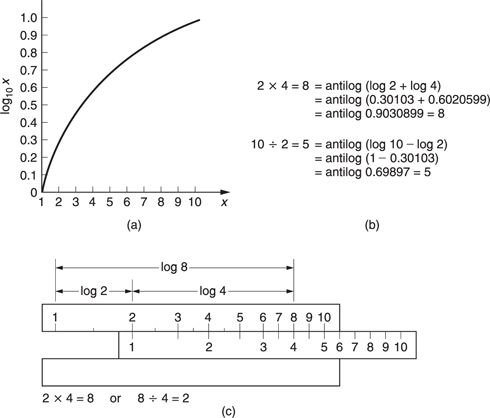
Figure 5.3 shows the principle of the logarithm. To give an example, if it is clear that 102 is 100 and 103 is 1000, then there must be a power between 2 and 3 to which 10 can be raised to give any value between 100 and 1000. That power is the logarithm to base 10 of the value. e.g. log10 300 = 2.5 approx. Note that 100 is 1.
Logarithms were developed by mathematicians before the availability of calculators or computers to ease calculations such as multiplication, squaring, division and extracting roots. The advantage is that armed with a set of log tables, multiplication can be performed by adding, division by subtracting. Figure 5.3 shows some examples. It will be clear that squaring a number is performed by adding two identical logs and the same result will be obtained by multiplying the log by 2.
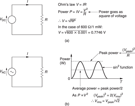
Figure 5.2 (a) Ohm’s law: the power developed in a resistor is proportional to the square of the voltage. Consequently, 1 mW in 600Ω requires 0.775V. With a sinusoidal alternating input (b), the power is a sine square function which can be averaged over one cycle. A DC voltage which would deliver the same power has a value which is the square root of the mean of the square of the sinusoidal input.
The slide rule is an early calculator which consists of two logarithmically engraved scales in which the length along the scale is proportional to the log of the engraved number. By sliding the moving scale, two lengths can easily be added or subtracted and as a result multiplication and division is readily obtained.
The logarithmic unit of measurement in telephones was called the Bel after Alexander Graham Bell, the inventor. Figure 5.4(a) shows that the Bel was defined as the log of the power ratio between the power to be measured and some reference power. Clearly the reference power must have a level of 0 Bels since log10 1 is 0.
The Bel was found to be an excessively large unit for many purposes and so it was divided into 10 deciBels, abbreviated to dB with a small d and a large B and pronounced ‘deebee’. Consequently the number of dB is ten times the log of the power ratio. A device such as an amplifier can have a fixed power gain which is independent of signal level and this can be measured in dB. However, when measuring the power of a signal, it must be appreciated that the dB is a ratio and to quote the number of dBs without stating the reference is about as senseless as describing the height of a mountain as 2000 without specifying whether this is feet or metres. To show that the reference is one milliWatt into 600O, the units will be dB(m). In radio engineering, the dB(W) will be found which is power relative to one Watt.
Although the dB(m) is defined as a power ratio, level measurements in audio are often done by measuring the signal voltage using 0.775 V as a reference in a circuit whose impedance is not necessarily 600O. Figure 5.4(b) shows that as the power is proportional to the square of the voltage, the power ratio will be obtained by squaring the voltage ratio. As squaring in logs is performed by doubling, the squared term of the voltages can be replaced by multiplying the log by a factor of two. To give a result in deciBels, the log of the voltage ratio now has to be multiplied by 20.
Whilst 600 O matched-impedance working is essential for the long distances encountered with telephones, it is quite inappropriate for analog audio wiring in the studio or the home. The wavelength of audio in wires at 20 kHz is 15 km. Most studios are built on a smaller scale than this and clearly analog audio cables are not transmission lines and their characteristic impedance is swamped by the devices connected at each end. Consequently the reader is cautioned that anyone who attempts to sell exotic analog audio cables by stressing their transmission line characteristics is more of a salesman than a physicist.
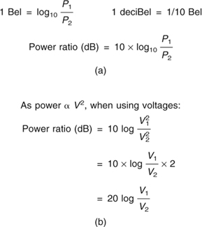
Figure 5.4 (a) The Bel is the log of the ratio between two powers, that to be measured and the reference. The Bel is too large so the deciBel is used in practice. (b) As the dB is defined as a power ratio, voltage ratios have to be squared. This is conveniently done by doubling the logs so the ratio is now multiplied by 20.
In professional analog audio systems impedance matching is not only unnecessary it is also undesirable. Figure 5.5(a) shows that when impedance matching is required the output impedance of a signal source must be artificially raised so that a potential divider is formed with the load. The actual drive voltage must be twice that needed on the cable as the potential divider effect wastes 6 dB of signal level and requires unnecessarily high power supply rail voltages in equipment. A further problem is that cable capacitance can cause an undesirable HF roll-off in conjunction with the high source impedance.
In modern professional analog audio equipment, shown in Figure 5.5(b) the source has the lowest output impedance practicable. This means that any ambient interference is attempting to drive what amounts to a short circuit and can only develop very small voltages. Furthermore, shunt capacitance in the cable has very little effect. The destination has a somewhat higher impedance (generally a few kO) to avoid excessive currents flowing and to allow several loads to be placed across one driver.
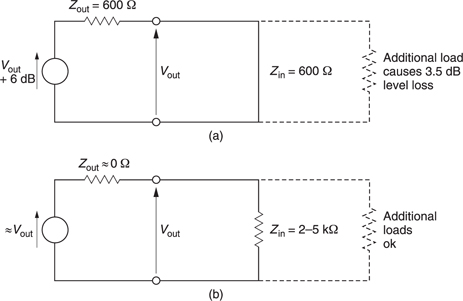
Figure 5.5 (a) Traditional impedance matched source wastes half the signal voltage in the potential divider due to the source impedance and the cable. (b) Modern practice is to use low-output impedance sources with high-impedance loads.(a) The Bel is the log of the ratio between two powers, that to be measured and the reference. The Bel is too large so the deciBel is used in practice. (b) As the dB is defined as a power ratio, voltage ratios have to be squared. This is conveniently done by doubling the logs so the ratio is now multiplied by 20.
In the absence of a fixed impedance it is now meaningless to consider power. Consequently only signal voltages are measured. The reference remains at 0.775V, but power and impedance are irrelevant. Voltages measured in this way are expressed in dB(u); the commonest unit of level in modern systems. Most installations boost the signals on interface cables by 4 dB. As the gain of receiving devices is reduced by 4 dB, the result is a useful noise advantage without risking distortion due to the drivers having to produce high voltages.
In order to make the difference between dB(m) and dB(u) clear, consider the lossless matching transformer shown in Figure 5.6. The turns ratio is 2:1 therefore the impedance matching ratio is 4:1. As there is no loss in the transformer, the power in is the same as the power out so that the transformer shows a gain of 0 dB(m). However, the turns ratio of 2:1 provides a voltage gain of 6 dB(u). The doubled output voltage will develop the same power into the quadrupled load impedance.
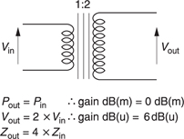
Figure 5.6 A lossless transformer has no power gain so the level in dB(m) on input and output is the same. However, there is a voltage gain when measurements are made in dB(u).
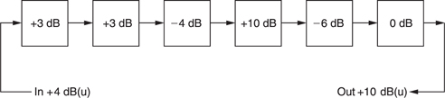
In a complex system signals may pass through a large number of processes, each of which may have a different gain. Figure 5.7 shows that if one stays in the linear domain and measures the input level in volts rms, the output level will be obtained by multiplying by the gains of all the stages involved. This is a complex calculation.
The difference between the signal level with and without the presence of a device in a chain is called the insertion loss measured in dB. However, if the input is measured in dB(u), the output level of the first stage can be obtained by adding the insertion loss in dB. The output level of the second stage can be obtained by further adding the loss of the second stage in dB and so on. The final result is obtained by adding together all of the insertion losses in dB and adding them to the input level in dB(u) to give the output level in dB(u). As the dB is a pure ratio it can multiply anything (by addition of logs) without changing the units. Thus dB(u) of level added to dB of gain are still dB(u).
In acoustic measurements, the sound pressure level (SPL) is measured in deciBels relative to a reference pressure of 2 × 10⁻⁵ Pascals (Pa) rms. In order to make the reference clear the units are dB(SPL). In measurements which are intended to convey an impression of subjective loudness, a weighting filter is used prior to the level measurement which reproduces the frequency response of human hearing which is most sensitive in the midrange. The most common standard frequency response is the so-called A-weighting filter, hence the term dB(A) used when a weighted level is being measured. At high or low frequencies, a lower reading will be obtained in dB(A) than in dB(SPL).
5.3 Audio level metering
There are two main reasons for having level meters in audio equipment: to line up or adjust the gain of equipment, and to assess the amplitude of the program material. Gain line-up is especially important in digital systems where an incorrect analog level can result in ADC clipping.
Line-up is often done using a 1 kHz sine wave generated at an agreed level such as 0 dB(u). If a receiving device does not display the same level, then its input sensitivity must be adjusted. Tape recorders and other devices which pass signals through are usually lined up so that their input and output levels are identical, i.e. their insertion loss is 0 dB. Lineup is important in large systems because it ensures that inadvertent level changes do not occur.
In measuring the level of a sine wave for the purposes of line-up, the dynamics of the meter are of no consequence, whereas on program material the dynamics matter a great deal. The simplest (and cheapest) level meter is essentially an AC voltmeter with a logarithmic response. As the ear is logarithmic, the deflection of the meter is roughly proportional to the perceived volume, hence the term Volume Unit (VU) meter.
In audio recording and broadcasting, the worst sin is to overmodulate the tape, the ADC or the transmitter by allowing a signal of excessive amplitude to pass. Real audio signals are rich in short transients which pass before the sluggish VU meter responds. Consequently the VU meter is also called the virtually useless meter in professional circles.
Broadcasters developed the peak program meter (PPM) which is also logarithmic, but which is designed to respond to peaks as quickly as the ear responds to distortion. Consequently the attack time of the PPM is carefully specified. If a peak is so short that the PPM fails to indicate its true level, the resulting overload will also be so brief that the HAS will not hear it. A further feature of the PPM is that the decay time of the meter is very slow, so that any peaks are visible for much longer and the meter is easier to read because the meter movement is less violent.
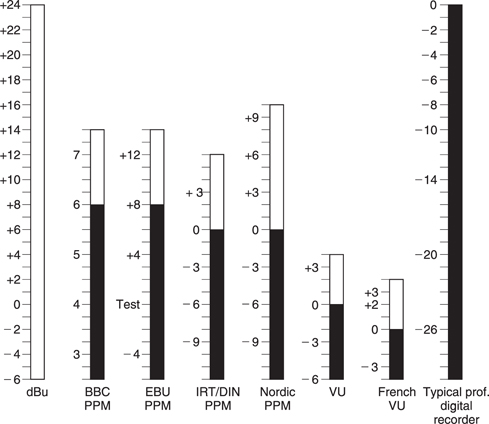
The original PPM as developed by the BBC was sparsely calibrated, but other users have adopted the same dynamics and added dB scales. Figure 5.8 shows some of the scales in use.
In broadcasting, the use of level metering and line-up procedures ensures that the level experienced by the viewer/listener does not change significantly from program to program. Consequently in a transmission suite, the goal would be to broadcast tapes at a level identical to that which was obtained during production. However, when making a recording prior to any production process, the goal would be to modulate the tape as fully as possible without clipping, as this would then give the best signal-to-noise ratio. The level would then be reduced if necessary in the production process.
Unlike analog recorders, digital systems do not have headroom, as there is no progressive onset of distortion until convertor clipping, the equivalent of saturation, occurs at 0 dBFs. Accordingly many digital recorders have level meters which read in dBFs. The scales are marked with 0 at the clipping level and all operating levels are below that. This causes no dificulty provided the user is aware of the consequences.
However, in the situation where a digital copy of an analog tape is to be made, it is very easy to set the input gain of the digital recorder so that line-up tone from the analog tape reads 0 dB. This lines up digital clipping with the analog operating level. When the tape is dubbed, all signals in the headroom suffer convertor clipping.
In order to prevent such problems, manufacturers and broadcasters have introduced artificial headroom on digital level meters, simply by calibrating the scale and changing the analog input sensitivity so that 0 dB analog is some way below clipping. Unfortunately there has been little agreement on how much artificial headroom should be provided, and machines which have it are seldom labelled with the amount. There is an argument which suggests that the amount of headroom should be a function of the sample wordlength, but this causes difficulties when transferring from one wordlength to another. In sixteen-bit working, 12 dB of headroom is a useful figure, but now that eighteen- and twentybit convertors are available, 18 dB may be more appropriate.
5.4 The ear
The human auditory system, the sense called hearing, is based on two obvious tranducers at the side of the head, and a number of less obvious mental processes which give us an impression of the world around us based on disturbances to the equilibrium of the air which we call sound. It is only possible briefly to introduce the subject here. The interested reader is referred to Moore2 for an excellent treatment.
The HAS can tell us, without aid from any other senses, where a sound source is, how big it is, whether we are in an enclosed space and how big that is. If the sound source is musical, we can further establish information such as pitch and timbre, attack, sustain and decay. In order to do this, the auditory system must work in the time, frequency and space domains. A sound reproduction system which is inadequate in one of these domains will be unrealistic however well the other two are satisfied. Chapter 3 introduced the concept of uncertainty between the time and frequency domains and the ear cannot analyse both at once. The HAS circumvents this by changing its characteristics dynamically so that it can concentrate on one domain or the other.
The acuity of the HAS is astonishing. It can detect tiny amounts of distortion, and will accept an enormous dynamic range over a wide number of octaves. If the ear detects a different degree of impairment between two audio systems and an original or ‘live’ sound in properly conducted tests, we can say that one of them is superior. Thus quality is completely subjective and can only be checked by listening tests. However, any characteristic of a signal which can be heard can, in principle, also be measured by a suitable instrument although in general the availability of such instruments lags the requirement and the use of such instruments lags the availability. The subjective tests will tell us how sensitive the instrument should be. Then the objective readings from the instrument give an indication of how acceptable a signal is in respect of that characteristic.
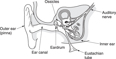
Figure 5.9 shows that the structure of the ear is traditionally divided into the outer, middle and inner ears. The outer ear works at low impedance, the inner ear works at high impedance, and the middle ear is an impedance-matching device. The visible part of the outer ear is called the pinna which plays a subtle role in determining the direction of arrival of sound at high frequencies. It is too small to have any effect at low frequencies. Incident sound enters the auditory canal or meatus. The pipe-like meatus causes a small resonance at around 4 kHz. Sound vibrates the eardrum or tympanic membrane which seals the outer ear from the middle ear. The inner ear or cochlea works by sound travelling though a fluid. Sound enters the cochlea via a membrane called the oval window. If airborne sound were to be incident on the oval window directly, the serious impedance mismatch would cause most of the sound to be reflected. The middle ear remedies that mismatch by providing a mechanical advantage.
The tympanic membrane is linked to the oval window by three bones known as ossicles which act as a lever system such that a large displacement of the tympanic membrane results in a smaller displacement of the oval window but with greater force. Figure 5.10 shows that the malleus applies a tension to the tympanic membrane rendering it conical in shape. The malleus and the incus are firmly joined together to form a lever. The incus acts upon the stapes through a spherical joint. As the area of the tympanic membrane is greater than that of the oval window, there is a further multiplication of the available force.
Consequently small pressures over the large area of the tympanic membrane are converted to high pressures over the small area of the oval window. The middle ear evolved to operate at natural sound levels and causes distortion at the high levels which can be generated with artificial amplification.
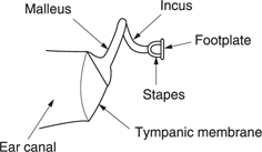
Figure 5.10 The malleus tensions the tympanic membrane into a conical shape. The ossicles provide an impedance-transforming lever system between the tympanic membrane and the oval.
The middle ear is normally sealed, but ambient pressure changes will cause static pressure on the tympanic membrane which is painful. The pressure is relieved by the Eustachian tube which opens involuntarily while swallowing. Some of the discomfort of the common cold is due to these tubes becoming blocked. The Eustachian tubes open into the cavities of the head and must normally be closed to avoid one’s own speech appearing deafeningly loud.
The ossicles are located by minute muscles which are normally relaxed. However, the middle ear reflex is an involuntary tightening of the tensor tympani and stapedius muscles which heavily damp the ability of the tympanic membrane and the stapes to transmit sound by about 12 dB at frequencies below 1 kHz. The main function of this reflex is to reduce the audibility of one’s own speech. However, loud sounds will also trigger this reflex which takes some 60–120 ms to operate; too late to protect against transients such as gunfire.
The cochlea is the transducer proper, converting pressure variations in the fluid into nerve impulses. However, unlike a microphone, the nerve impulses are not an analog of the incoming waveform. Instead the cochlea has some analysis capability which is combined with a number of mental processes to make a complete analysis. As shown in Figure 5.11(a), the cochlea is a fluid-filled tapering spiral cavity within bony walls. The widest part, near the oval window, is called the base and the distant end is the apex. Figure 5.11(b) shows that the cochlea is divided lengthwise into three volumes by Reissner’s membrane and the basilar membrane. The scala vestibuli and the scala tympani are connected by a small aperture at the apex of the cochlea known as the helicotrema. Vibrations from the stapes are transferred to the oval window and become fluid pressure variations which are relieved by the flexing of the round window.
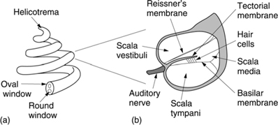
Figure 5.11 (a) The cochlea is a tapering spiral cavity. (b) The cross-section of the cavity is divided by Reissner’s membrane and the basilar membrane.
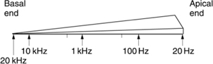
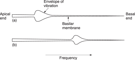
Figure 5.12 The basilar membrane tapers so its resonant frequency changes along its length.
Effectively the basilar membrane is in series with the fluid motion and is driven by it except at very low frequencies where the fluid flows through the helicotrema, decoupling the basilar membrane.
To assist in its frequency-domain operation, the basilar membrane is not uniform. Figure 5.12 shows that it tapers in width and varies in thickness in the opposite sense to the taper of the cochlea. The part of the basilar membrane which resonates as a result of an applied sound is a function of the frequency. High frequencies cause resonance near to the oval window, whereas low frequencies cause resonances further away. More precisely the distance from the apex where the maximum resonance occurs is a logarithmic function of the frequency. Consequently tones spaced apart in octave steps will excite evenly spaced resonances in the basilar membrane. The prediction of resonance at a particular location on the membrane is called place theory. Among other things, the basilar membrane is a mechanical frequency analyser. A knowledge of the way it operates is essential to an understanding of musical phenomena such as pitch discrimination, timbre, consonance and dissonance and to auditory phenomena such as critical bands, masking and the precedence effect.
The vibration of the basilar membrane is sensed by the organ of Corti which runs along the centre of the cochlea. The organ of Corti is active in that it contains elements which can generate vibration as well as sense it. These are connected in a regenerative fashion so that the Q factor, or frequency selectivity, of the ear is higher than it would otherwise be. The deflection of hair cells in the organ of Corti triggers nerve firings and these signals are conducted to the brain by the auditory nerve.
Nerve firings are not a perfect analog of the basilar membrane motion. A nerve firing appears to occur at a constant phase relationship to the basilar vibration; a phenomenon called phase locking, but firings do not necessarily occur on every cycle. At higher frequencies firings are intermittent, yet each is in the same phase relationship.
The resonant behaviour of the basilar membrane is not observed at the lowest audible frequencies below 50 Hz. The pattern of vibration does not appear to change with frequency and it is possible that the frequency is low enough to be measured directly from the rate of nerve firings.
5.5 Level and loudness
At its best, the HAS can detect a sound pressure variation of only 2 × 10⁻⁵ Pascals rms and so this figure is used as the reference against which sound pressure level (SPL) is measured. The sensation of loudness is a logarithmic function of SPL hence the use of the deciBel explained in section 5.2. The dynamic range of the HAS exceeds 130 dB, but at the extremes of this range, the ear is either straining to hear or is in pain.
The frequency response of the HAS is not at all uniform and it also changes with SPL. The subjective response to level is called loudness and is measured in phons. The phon scale and the SPL scale coincide at 1 kHz, but at other frequencies the phon scale deviates because it displays the actual SPLs judged by a human subject to be equally loud as a given level at 1 kHz. Figure 5.13 shows the so-called equal loudness contours which were originally measured by Fletcher and Munson and subsequently by Robinson and Dadson. Note the irregularities caused by resonances in the meatus at about 4 kHz and 13 kHz.
Usually, people’s ears are at their most sensitive between about 2 kHz and 5 kHz, and although some people can detect 20 kHz at high level, there is much evidence to suggest that most listeners cannot tell if the upper frequency limit of sound is 20 kHz or 16 kHz.3,4 For a long time it was thought that frequencies below about 40 Hz were unimportant, but it is now clear that reproduction of frequencies down to 20 Hz improves reality and ambience.5 The generally accepted frequency range for highquality audio is 20–20 000 Hz, although for broadcasting an upper limit of 15 000 Hz is often applied.
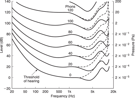
Figure 5.13 Contours of equal loudness showing that the frequency response of the ear is highly level dependent (solid line. age 20; dashed line, age 60).
The most dramatic effect of the curves of Figure 5.13 is that the bass content of reproduced sound is disproportionately reduced as the level is turned down. This would suggest that if a powerful yet high-quality reproduction system is available the correct tonal balance when playing a good recording can be obtained simply by setting the volume control to the correct level. This is indeed the case. A further consideration is that many musical instruments and the human voice change timbre with level and there is only one level which sounds correct for the timbre.
Oddly, there is as yet no standard linking the signal level in a transmission or recording system with the SPL at the microphone, although with the advent of digital microphones this useful information could easily be sent as metadata.
Loudness is a subjective reaction and is almost impossible to measure. In addition to the level-dependent frequency response problem, the listener uses the sound not for its own sake but to draw some conclusion about the source. For example, most people hearing a distant motorcycle will describe it as being loud. Clearly at the source, it is loud, but the listener has compensated for the distance. Paradoxically the same listener may then use a motor mower without hearing protection.
The best that can be done is to make some compensation for the leveldependent response using weighting curves. Ideally there should be many, but in practice the A, B and C weightings were chosen where the A curve is based on the 40-phon response. The measured level after such a filter is in units of dBA. The A curve is almost always used because it most nearly relates to the annoyance factor of distant noise sources. The use of A-weighting at higher levels is highly questionable.
5.6 Frequency discrimination
Figure 5.14 shows an uncoiled basilar membrane with the apex on the left so that the usual logarithmic frequency scale can be applied. The envelope of displacement of the basilar membrane is shown for a single frequency at (a). The vibration of the membrane in sympathy with a single frequency cannot be localized to an infinitely small area, and nearby areas are forced to vibrate at the same frequency with an amplitude that decreases with distance. Note that the envelope is asymmetrical because the membrane is tapering and due to frequencydependent losses in the propagation of vibrational energy down the cochlea. If the frequency is changed, as in (b), the position of maximum displacement will also change. As the basilar membrane is continuous, the position of maximum displacement is infinitely variable, allowing extremely good pitch discrimination of about one twelfth of a semitone which is determined by the spacing of hair cells.
In the presence of a complex spectrum, the finite width of the vibration envelope means that the ear fails to register energy in some bands when there is more energy in a nearby band. Within those areas, other frequencies are mechanically excluded because their amplitude is insufficient to dominate the local vibration of the membrane. Thus the Q factor of the membrane is responsible for the degree of auditory masking, defined as the decreased audibility of one sound in the presence of another.
The term used in psychoacoustics to describe the finite width of the vibration envelope is critical bandwidth. Critical bands were first described by Fletcher.6 The envelope of basilar vibration is a complicated function. It is clear from the mechanism that the area of the membrane involved will increase as the sound level rises. Figure 5.15 shows the bandwidth as a function of level.
As was shown in Chapter 3, the Heisenberg inequality teaches that the higher the frequency resolution of a transform, the worse the time accuracy. As the basilar membrane has finite frequency resolution measured in the width of a critical band, it follows that it must have finite time resolution. This also follows from the fact that the membrane is resonant, taking time to start and stop vibrating in response to a stimulus. There are many examples of this. Figure 5.16 shows the impulse response and Figure 5.17 the perceived loudness of a tone burst increases with duration up to about 200 ms due to the finite response time.
The HAS has evolved to offer intelligibility in reverberant environments which it does by averaging all received energy over a period of about 30 ms. Reflected sound which arrives within this time is integrated to produce a louder sensation, whereas reflected sound which arrives after that time can be temporally discriminated and is perceived as an echo. Microphones have no such ability which is why we often need to have acoustic treatment in areas where microphones are used.
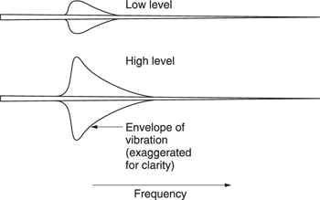
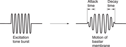
Figure 5.16 Impulse response of the ear showing slow attack and decay due to resonantbehaviour.
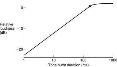
Figure 5.17 Perceived level of tone burst rises with duration as resonance builds up.
A further example of the finite time discrimination of the HAS is the fact that short interruptions to a continuous tone are difficult to detect. Finite time resolution means that masking can take place even when the masking tone begins after and ceases before the masked sound. This is referred to as forward and backward masking.7
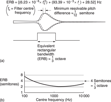
As the vibration envelope is such a complicated shape, Moore and Glasberg have proposed the concept of equivalent rectangular bandwidth to simplify matters. The ERB is the bandwidth of a rectangular filter which passes the same power as a critical band. Figure 5.18(a) shows the expression they have derived linking the ERB with frequency. This is plotted in (b) where it will be seen that one third of an octave is a good approximation. This is about thirty times broader than the pitch discrimination also shown in (b).
Figure 5.19 shows an electrical signal (a) in which two equal sine waves of nearly the same frequency have been linearly added together. Note that the envelope of the signal varies as the two waves move in and out of phase. Clearly the frequency transform calculated to infinite accuracy is that shown at (b). The two amplitudes are constant and there is no evidence of the envelope modulation. However, such a measurement requires an infinite time. When a shorter time is available, the frequency discrimination of the transform falls and the bands in which energy is detected become broader.
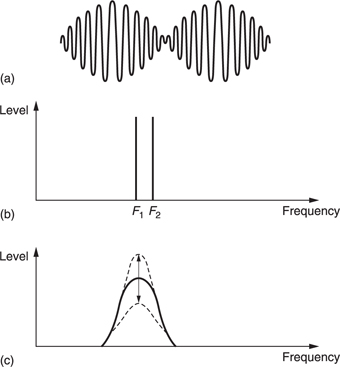
When the frequency discrimination is too wide to distinguish the two tones as in (c), the result is that they are registered as a single tone. The amplitude of the single tone will change from one measurement to the next because the envelope is being measured. The rate at which the envelope amplitude changes is called a beat frequency which is not actually present in the input signal. Beats are an artifact of finite frequency resolution transforms. The fact that the HVS produces beats from pairs of tones proves that it has finite resolution.
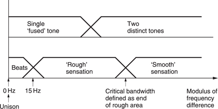
Measurement of when beats occur allows measurement of critical bandwidth. Figure 5.20 shows the results of human perception of a twotone signal as the frequency dF difference changes. When dF is zero, described musically as unison, only a single note is heard. As dF increases, beats are heard, yet only a single note is perceived. The limited frequency resolution of the basilar membrane has fused the two tones together. As dF increases further, the sensation of beats ceases at 12–15 Hz and is replaced by a sensation of roughness or dissonance. The roughness is due to parts of the basilar membrane being unable to decide the frequency at which to vibrate. The regenerative effect may well become confused under such conditions. The roughness which persists until dF has reached the critical bandwidth beyond which two separate tones will be heard because there are now two discrete basilar resonances. In fact this is the definition of critical bandwidth.
5.7 Music and the ear
The characteristics of the HVS, especially critical bandwidth, are responsible for the way music has evolved. Beats are used extensively in music. When tuning a pair of instruments together, a small tuning error will result in beats when both play the same nominal note. In certain pipe organs, pairs of pipes are sounded together with a carefully adjusted pitch error which results in a pleasing tremolo effect.
With certain exceptions, music is intended to be pleasing and so dissonance is avoided. Two notes which sound together in a pleasing manner are described as harmonious or consonant. Two sine waves appear consonant if they separated by a critical bandwidth because the roughness of Figure 5.20 is avoided, but real musical instruments produce a series of harmonics in addition to the fundamental.
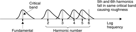
Figure 5.21 shows the spectrum of a harmonically rich instrument. The fundamental and the first few harmonics are separated by more than a critical band, but from the seventh harmonic more than one harmonic will be in one band and it is possible for dissonance to occur. Musical instruments have evolved to avoid the production of seventh and higher harmonics. Violins and pianos are played or designed to excite the strings at a node of the seventh harmonic to suppress this dissonance.
Harmonic distortion in audio equipment is easily detected even in minute quantities because the first few harmonics fall in non-overlapping critical bands. The sensitivity of the HAS to third harmonic distortion probably deserves more attention in audio equipment than the fidelity of the dynamic range or frequency response.
When two harmonically rich notes are sounded together, the harmonics will fall within the same critical band and cause dissonance unless the fundamentals have one of a limited number of simple relationships which makes the harmonics fuse. Clearly an octave relationship is perfect.
Figure 5.22 shows some examples. In (a) two notes with the ratio (interval) 3:2 are considered. The harmonics are either widely separated or fused and the combined result is highly consonant. The interval of 3:2 is known to musicians as a perfect fifth. In (b) the ratio is 4:3. All harmonics are either at least a third of an octave apart or are fused. This relationship is known as a perfect fourth. The degree of dissonance over the range from 1:1 to 2:1 (unison to octave) was investigated by Helmholtz and is shown in Figure 5.22(c). Note that the dissonance rises at both ends where the fundamentals are within a critical bandwidth of one another. Dissonances in the centre of the scale are where some harmonics lie in a within a critical bandwidth of one another. Troughs in the curve indicate areas of consonance. Many of the troughs are not very deep, indicating that the consonance is not perfect. This is because of the effect shown in Figure 5.21 in which high harmonics get closer together with respect to critical bandwidth. When the fundamentals are closer together, the harmonics will become dissonant at a lower frequency, reducing the consonance. Figure 5.22(c) also shows the musical terms used to describe the consonant intervals.
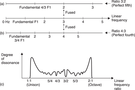
Figure 5.22 (a) Perfect fifth with a frequency ratio of 3:2 is consonant because harmonics are either in different critical bands or are fused. (b) Perfect fourth achieves the same result with 4:3 frequency ratio. (c) Degree of dissonance over range from 1:1 to 2:1.
It is clear from Figure 5.22(c) that the notes of the musical scale have empirically been established to allow the maximum consonance with pairs of notes and chords. Early instruments were tuned to the just diatonic scale in exactly this way. Unfortunately the just diatonic scale does not allow changes of key because the notes are not evenly spaced. A key change is where the frequency of every note in a piece of music is multiplied by a constant, often to bring the accompaniment within the range of a singer. In continuously tuned instruments such as the violin and the trombone this is easy, but with fretted or keyboard instruments such as a piano there is a problem.
The equal-tempered scale is a compromise between consonance and key changing. The octave is divided into twelve equal intervals called tempered semitones. On a keyboard, seven of the keys are white and produce notes very close to those of the just diatonic scale, and five of the keys are black. Music can be transposed in semitone steps by using the black keys. Figure 5.23 shows an example of transposition where a scale is played in several keys.
Frequency is an objective measure whereas pitch is the subjective near equivalent. Clearly frequency and level are independent, whereas pitch and level are not. Figure 5.24 shows the relationship between pitch and level. Place theory indicates that the hearing mechanism can sense a single frequency quite accurately as a function of the place or position of maximum basilar vibration. However, most periodic sounds and real musical instruments produce a series of harmonics in addition to the fundamental. When a harmonically rich sound is present the basilar membrane is excited at spaced locations. Figure 5.25(a) shows all harmonics, (b) shows even harmonics predominating and (c) shows odd harmonics predominating. It would appear that the HAS is accustomed to hearing harmonics in various amounts and the consequent regular pattern of excitation. It is the overall pattern which contributes to the sensation of pitch even if individual partials vary enormously in relative level.
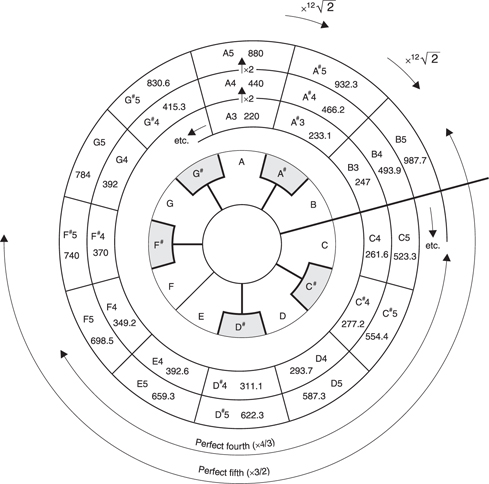
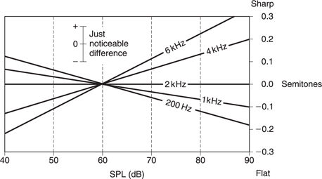
Figure 5.24 Pitch sensation is a function of level.
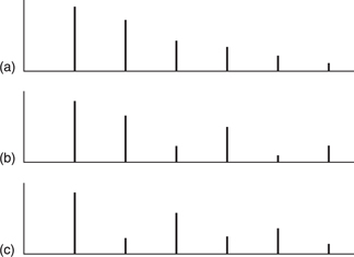
Experimental signals in which the fundamental has been removed leaving only the harmonics result in unchanged pitch perception. The pattern in the remaining harmonics is enough uniquely to establish the missing fundamental. Imagine the fundamental in (b) to be absent. Neither the second harmonic nor the third can be mistaken for the fundamental because if they were fundamentals a different pattern of harmonics would result. A similar argument can be put forward in the time domain, where the timing of phase-locked nerve firings responding to a harmonic will periodically coincide with the nerve firings of the fundamental. The ear is used to such time patterns and will use them in conjunction with the place patterns to determine the right pitch. At very low frequencies the place of maximum vibration does not move with frequency yet the pitch sensation is still present because the nerve firing frequency is used.
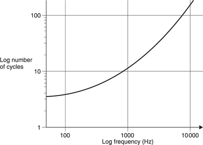
As the fundamental frequency rises it is difficult to obtain a full pattern of harmonics as most of them fall outside the range of hearing. The pitch discrimination ability is impaired and needs longer to operate. Figure 5.26 shows the number of cycles of excitation needed to discriminate pitch as a function of frequency. Clearly at around 5 kHz performance is failing because there are hardly any audible harmonics left. Phase locking also fails at about the same frequency. Musical instruments have evolved accordingly, with the highest notes of virtually all instruments found below 5 kHz.
5.8 The physics of sound
Sound is simply an airborne version of vibration which is why the two topics are inextricably linked. The air which carries sound is a mixture of gases, mostly nitrogen, some oxygen, a little carbon dioxide and so on. Gases are the highest energy state of matter, which is another way of saying that you have to heat ice to get water then heat it some more to get steam. The reason that a gas takes up so much more room than a liquid is that the molecules contain so much energy that they break free from their neighbours and rush around at high speed. As Figure 5.27(a) shows, the innumerable elastic collisions of these high-speed molecules produce pressure on the walls of any gas container. In fact the distance a molecule can go without a collision, the mean-free path, is quite short at atmospheric pressure. Consequently gas molecules also collide with each other elastically, so that if left undisturbed, in a container at a constant temperature, every molecule would end up with essentially the same energy and the pressure throughout would be constant and uniform.
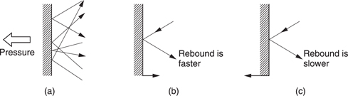
Figure 5.27 (a) The pressure exerted by a gas is due to countless elastic collisions between gas molecules and the walls of the container. (b) If the wall moves against the gas pressure, the rebound velocity increases. (c) Motion with the gas pressure reduces the particle velocity.
Sound disturbs this simple picture. Figure 5.27(b) shows that a solid object which moves against gas pressure increases the velocity of the rebounding molecules, whereas in Figure 5.27(c) one moving with gas pressure reduces that velocity. The average velocity and the displacement of all the molecules in a layer of air near to a moving body is the same as the velocity and displacement of the body. Movement of the body results in a local increase or decrease in pressure of some kind. Thus sound is both a pressure and a velocity disturbance. Integration of the velocity disturbance gives the displacement.
Despite the fact that a gas contains endlessly rushing colliding molecules, a small mass or particle of gas can have stable characteristics because the molecules leaving are replaced by new ones with identical statistics. As a result, acoustics seldom considers the molecular structure of air and the constant motion is neglected. Thus when particle velocity and displacement is considered in acoustics, this refers to the average values of a large number of molecules. The undisturbed container of gas referred to earlier will have a particle velocity and displacement of zero at all points.
When the volume of a fixed mass of gas is reduced, the pressure rises. The gas acts like a spring. However, a gas also has mass. Sound travels through air by an interaction between the mass and the springiness. Imagine pushing a mass via a spring. It would not move immediately because the spring would have to be compressed in order to transmit a force. If a second mass is connected to the first by another spring, it would start to move even later. Thus the speed of a disturbance in a mass/spring system depends on the mass and the stiffness.
After the disturbance had propagated the masses would return to their rest position. The mass/spring analogy is helpful for an early understanding, but is too simple to account for commonly encountered acoustic phenomena such as spherically expanding waves. It must be remembered that the mass and stiffness are distributed throughout the gas in the same way that inductance and capacitance are distributed in a transmission line. Sound travels through air without a net movement of the air.
Unlike solids, the elasticity of gas is a complicated process. If a fixed mass of gas is compressed, work has to be done on it. This will create heat in the gas. If the heat is allowed to escape and the compression does not change the temperature, the process is said to be isothermal. However, if the heat cannot escape the temperature will rise and give a disproportionate increase in pressure. This process is said to be adiabatic and the Diesel engine depends upon it. In most audio cases there is insufficient time for much heat transfer and so air is considered to act adiabatically. Figure 5.28 shows how the speed of sound c in air can be derived by calculating its elasticity under adiabatic conditions.
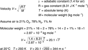
If the volume allocated to a given mass of gas is reduced isothermally, the pressure and the density will rise by the same amount so that c does not change. If the temperature is raised at constant pressure, the density goes down and so the speed of sound goes up. Gases with lower density than air have a higher speed of sound. Divers who breathe a mixture of oxygen and helium to prevent ‘the bends’ must accept that the pitch of their voices rises remarkably. Digital pitch shifters can be used to facilitate communication. The speed of sound is proportional to the square root of the absolute temperature. Temperature changes with respect to absolute zero (–273°C) also amount to around 1 per cent except in extremely inhospitable places.
The speed of sound experienced by most of us is about 1000 feet per second or 344 metres per second. Temperature falls with altitude in the atmosphere and with it the speed of sound. The local speed of sound is defined as Mach 1. Consequently supersonic aircraft are fitted with Mach meters.
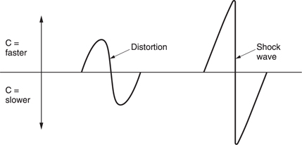
As air acts adiabatically, a propagating sound wave causes cyclic temperature changes. The speed of sound is a function of temperature, yet sound causes a temperature variation. One might expect some effects because of this. Fortunately, sounds which are below the threshold of pain have such a small pressure variation compared with atmospheric pressure that the effect is negligible and air can be assumed to be linear. However, on any occasion where the pressures are higher, this is not a valid assumption. In such cases the positive half-cycle significantly increases local temperature and the speed of sound, whereas the negative half-cycle reduces temperature and velocity. Figure 5.29 shows that this results in significant distortion of a sine wave, ultimately causing a shock wave which can travel faster than the speed of sound until the pressure has dissipated with distance. This effect is responsible for the sharp sound of a handclap.
This behaviour means that the speed of sound changes slightly with frequency. High frequencies travel slightly faster than low because there is less time for heat conduction to take place. Figure 5.30 shows that a complex sound source produces harmonics whose phase relationship with the fundamental advances with the distance the sound propagates. This allows one mechanism (there are others) by which the HAS can judge the distance from a known sound source. Clearly for realistic sound reproduction nothing in the audio chain must distort the phase relationship between frequencies. A system which accurately preserves such relationships is said to display linear phase.
Sound can be due to a one-off event known as percussion, or a periodic event such as the sinusoidal vibration of a tuning fork. The sound due to percussion is called transient whereas a periodic stimulus produces steady-state sound having a frequency f.
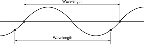
Because sound travels at a finite speed, the fixed observer at some distance from the source will experience the disturbance at some later time. In the case of a transient, the observer will detect a single replica of the original as it passes at the speed of sound. In the case of the tuning fork, a periodic sound, the pressure peaks and dips follow one another away from the source at the speed of sound. For a given rate of vibration of the source, a given peak will have propagated a constant distance before the next peak occurs. This distance is called the wavelength,λ. Figure 5.31 shows that wavelength is defined as the distance between any two identical points on the whole cycle. If the source vibrates faster, successive peaks get closer together and the wavelength gets shorter. Wavelength is inversely proportional to the frequency. It is easy to remember that the wavelength of 1000 Hz is a foot (about 30 cm).
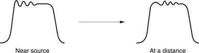
Figure 5.30 In a complex waveform, high frequencies travel slightly faster producing a relative phase change with distance.
If there is relative motion between the source and the observer, the frequency of a periodic sound will be changed. Figure 5.32 shows a sound source moving towards the observer. At the end of a cycle, the source will be nearer the observer than at the beginning of the cycle. As a result the wavelength radiated in the direction of the observer will be shortened so that the pitch rises. The wavelength of sounds radiated away from the observer will be lengthened. The same effect will occur if the observer moves. This is the Doppler effect, which is most noticeable on passing motor vehicles whose engine notes appear to drop as they pass. Note that the effect always occurs, but it is only noticeable on a periodic sound. Where the sound is aperiodic, such as broadband noise, the Doppler shift will not be heard.
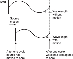
Figure 5.32 Periodic sounds are subject to Doppler shift if there is relative motion between the source and the observer.
Sound is a wave motion, and the way a wave interacts with any object depends upon the relative size of that object and the wavelength. The audible range of wavelengths is from around 17 millimetres to 17 metres so dramatic changes in the behaviour of sound over the frequency range should be expected.
Figure 5.33(a) shows that when the wavelength of sound is large compared to the size of a solid body, the sound will pass around it almost as if it were not there. When the object is large compared to the wavelength, then simple reflection takes place as in Figure 5.33(b). However, when the size of the object and the wavelength are comparable, the result can only be explained by diffraction theory.
The parameter which is used to describe this change of behaviour with wavelength is known as the wave number k and is defined as:
![]()
where f = frequency, c = the speed of sound and λ = wavelength. In practice the size of any object or distance a in metres is multiplied by k.
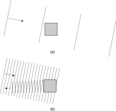
Figure 5.33 (a) Sound waves whose spacing is large compared to an obstacle simply pass round it. (b) When the relative size is reversed, an obstacle becomes a reflector.
A good rule of thumb is that below ka = 1, sound tends to pass around as in Figure 5.33(a) whereas above ka = 1, sound tends to reflect as in (b).
5.9 How sound is radiated
When sound propagates, there are changes in velocity v, displacement x and pressure p. Figure 5.34 shows that the velocity and the displacement are always in quadrature. This is obvious because velocity is the differential of the displacement. When the displacement reaches its maximum value and is on the point of reversing direction, the velocity is zero. When the displacement is zero the velocity is maximum.
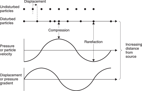
Figure 5.34 The pressure, velocity and displacement of particles as sound propagates.
The pressure and the velocity are linked by the acoustic impedance z which is given by p/v. Just like electrical impedances which can be reactive, the acoustic impedance is complex and varies with acoustic conditions. Consequently the phase relationship between velocity and pressure also varies. When any vibrating body is in contact with the air, a thin layer of air must have the same velocity as the surface of the body. The pressure which results from that velocity depends upon the acoustic impedance.
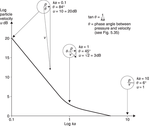
The wave number is useful to explain the way in which sound is radiated. Consider a hypothetical pulsating sphere as shown in Figure 5.35. The acoustic impedance changes with radius a. If the sphere pulsates very slowly, it will do work against air pressure as it expands and the air pressure will return the work as it contracts. There is negligible radiation because the impedance is reactive. Figure 5.35(a) shows that when ka is small there is a 90° phase shift between the pressure and the velocity. As the frequency or the radius rises, as in (b), the phase angle reduces from 90° and the pressure increases. When ka is large, the phase angle approaches zero and the pressure reaches its maximum value compared to the velocity. The impedance has become resistive.
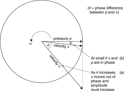
When ka is very large, the spherical radiator is at a distance and the spherical waves will have become plane waves. Figure 5.34 showed the relationships between pressure, velocity and displacement for a plane wave. A small air mass may have kinetic energy due to its motion and kinetic energy due to its compression. The total energy is constant, but the distribution of energy between kinetic and potential varies throughout the wave. This relationship will not hold when ka is small. This can easily occur especially at low frequencies where the wavelengths can be several metres.
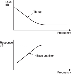
Microphones can transduce either the pressure or the velocity component of sound. When ka is large, the pressure and velocity waveforms in a spherical wave are identical. However it will be clear from Figure 5.35(a) and (b) that when ka is small the velocity exceeds the pressure component. This is the cause of the well-known proximity effect, also known as tip-up, which emphasizes low frequencies when velocitysensing microphones are used close to a sound source. Figure 5.36 shows the response of a velocity microphone relative to that of a pressure microphone for different values of ka. Various combinations of distance and frequency are given for illustration. Practical microphones often incorporate some form of bass-cut filter to offset the effect.
The sensation of sound is proportional to the average velocity. However, the displacement is the integral of the velocity. Figure 5.37 shows that to obtain an identical velocity or slope the amplitude must increase as the inverse of the frequency. Consequently for a given SPL low-frequency sounds result in much larger air movement than high frequency. The SPL is proportional to the volume velocity U of the source which is obtained by multiplying the vibrating area in m2 by the velocity in m/s. As SPL is proportional to volume velocity, as frequency falls the volume or displacement must rise. This means that low-frequency sound can only be radiated effectively by large objects, hence all the bass instruments in the orchestra are much larger than their treble equivalents. This is also the reason why a loudspeaker cone is only seen to move at low frequencies.

Figure 5.37 For a given velocity or slope, lower frequencies require greater amplitude.
The units of volume velocity are cubic metres per second and so sound is literally an alternating current. The pressure p is linked to the current by the impedance just as it is in electrical theory. There are direct analogies between acoustic and electrical parameters and equations which are helpful. One small difficulty is that whereas alternating electrical parameters are measured in rms units, acoustic units are not. Thus when certain acoustic parameters are multiplied together the product has to be divided by two. This happens automatically with rms units. Figure 5.38 shows the analogous equations.
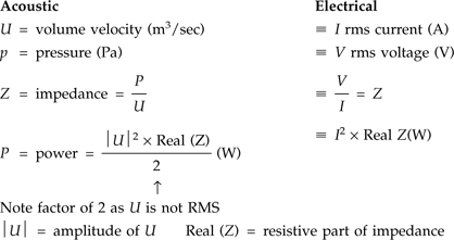
Figure 5.38 Electrical units are rms whereas many acoustic units are not, hence the factor of two difference in otherwise analogous equations.
The intensity of a sound is the sound power passing through unit area. In the far field it is given by the product of the volume velocity and the pressure. In the near field the relative phase angle will have to be considered. Intensity is a vector quantity as it has direction which is considered to be perpendicular to the area in question. The total sound power is obtained by multiplying the intensity by the cross-sectional area through which it passes. Power is a scalar quantity because it can be radiated in all directions.
When a spherical sound wave is considered, there is negligible loss as it advances outwards. Consequently the sound power passing through the surface of an imaginary sphere surrounding the source is independent of the radius of that sphere. As the area of a sphere is proportional to the square of the radius, it will be clear that the intensity falls according to an inverse square law.
The inverse square law should be used with caution. There are a number of exceptions. As was seen in Figure 5.36, the proximity effect causes a deviation from the inverse square law for small ka. The area in which there is deviation from inverse square behaviour is called the near field.
In reverberant conditions a sound field is set up by reflections. As the distance from the source increases at some point the level no longer falls.
It is also important to remember that the inverse square law applies only to near-point sources. A line source radiates cylindrically and intensity is then inversely proportional to radius. Noise from a busy road approximates to a cylindrical source.
5.10 Acoustics
A proper understanding of the behaviour of sound requires familiarity with the principles of wave acoustics. Wave theory is used in many different disciplines including radar, sonar, optics, antenna and filter design and the principles remain the same. Consequently the designer of a loudspeaker may obtain inspiration from studying a radar antenna or a CD pickup.
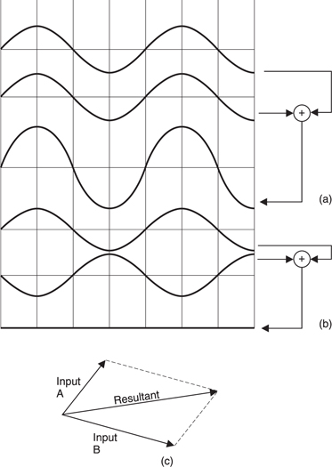
Figure 5.39 shows that when two sounds of equal amplitude and frequency add together, the result is completely dependent on the relative phase of the two. At (a) when the phases are identical, the result is the arithmetic sum. At (b) where there is a 180° relationship, the result is complete cancellation. This is constructive and destructive interference. At any other phase and/or amplitude relationship, the result can only be obtained by vector addition as shown in (c).
The wave theory of propagation of sound is based on interference and suggests that a wavefront advances because an infinite number of point sources can be considered to emit spherical waves which will only add when they are all in the same phase. This can only occur in the plane of the wavefront. Figure 5.40(a) shows that at all other angles, interference between spherical waves is destructive. For any radiating body, such as a vibrating object, it is easy to see from Figure 5.40(b) that when ka is small, only weak spherical radiation is possible, whereas when ka is large, a directional plane wave can be propagated or beamed. Consequently highfrequency sound behaves far more directionally than low-frequency sound.
When a wavefront arrives at a solid body, it can be considered that the surface of the body acts as an infinite number of points which reradiate the incident sound in all directions. It will be seen that when ka is large and the surface is flat, constructive interference only occurs when the wavefront is reflected such that the angle of reflection is the same as the angle of incidence. When ka is small, the amount of reradiation from the body compared to the radiation in the wavefront is very small. Constructive interference takes place beyond the body as if it were absent, thus it is correct to say that the sound diffracts around the body.
Figure 5.41 shows two identical sound sources which are spaced apart by a distance of several wavelengths and which vibrate in-phase. At all points equidistant from the sources the radiation adds constructively. The same is true where there are path length differences which are multiples of the wavelength. However, in certain directions the path length difference will result in relative phase reversal. Destructive interference means that sound cannot leave in those directions. The resultant diffraction pattern has a polar diagram which consists of repeating lobes with nulls between them.
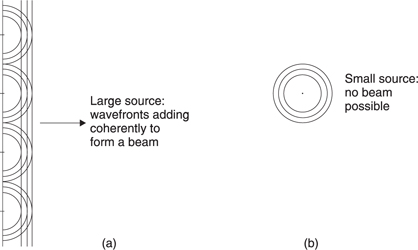
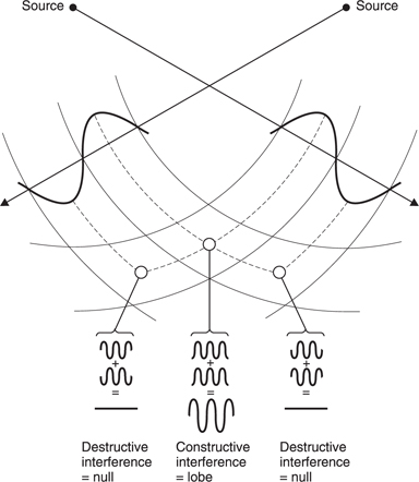
Figure 5.41 Constructive and destructive interference between two identical sources.
This chapter has so far considered only the radiation of a pulsating sphere; a situation which is too simple to model many real-life sound r adiators. The situation of Figure 5.41 can be extended to predict the results of vibrating bodies of arbitrary shape. Figure 5.42 shows a hypothetical rigid circular piston vibrating in an opening in a plane surface. This is apparently much more like a real loudspeaker. As it is rigid, all parts of it vibrate in the same phase. Following concepts advanced earlier, a rigid piston can be considered to be an infinite number of point sources. The result at an arbitrary point in space in front of the piston is obtained by integrating the waveform from every point source.
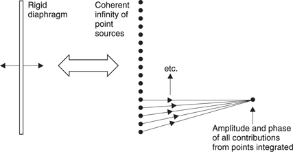
Figure 5.42 A rigid radiating surface can be considered as an infinity of coherent point sources. The result at a given location is obtained by integrating the radiation from each point.
A transducer can be affected dramatically by the presence of other objects, but the effect is highly frequency dependent. In Figure 5.43(a) a high frequency is radiated, and this simply reflects from the nearby object because the wavelength is short and the object is acoustically distant or in the far field. However, if the wavelength is made longer than the distance between the source and the object as in Figure 5.43(b), the object is acoustically close or in the near field and becomes part of the source. The effect is that the object reduces the solid angle into which radiation can take place as well as raising the acoustic impedance the transducer sees.
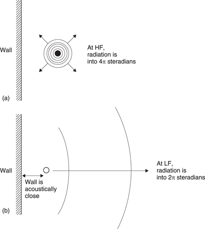
The volume velocity of the source is confined into a smaller crosssectional area and consequently the velocity must rise in inverse proportion to the solid angle.
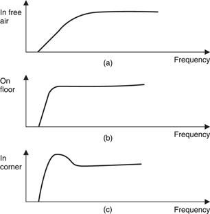
In Figure 5.44 the effect of positioning a loudspeaker is shown. In free space (a) the speaker might show a reduction in low frequencies which disappears when it is placed on the floor (b). In this case placing the speaker too close to a wall, or even worse, in a corner, (c), will emphasize the low-frequency output. High-quality loudspeakers will have an adjustment to compensate for positioning. The technique can be useful in the case of small cheap loudspeakers whose LF response is generally inadequate. Some improvement can be had by corner mounting.
It will be evident that at low frequencies the long wavelengths make it impossible for two close-spaced radiators acoustically to get out of phase. Consequently when two radiators are working within one another’s near field, they act like a single radiator. Each radiator will experience a doubled acoustic impedance because of the presence of the other. Thus the pressure for a given volume velocity will be doubled. As the intensity is proportional to the square of the pressure, it will be quadrupled.
The effect has to be taken into account when stereo loudspeakers are installed. At low frequencies the two speakers will be acoustically close and so will mutually raise their acoustic impedance causing a potential bass tip-up problem. When a pair of stereo speakers has been properly equalized, disconnecting one will result in the remaining speaker sounding bass light. In surround-sound systems there may be four or five speakers working in one another’s near field at low frequencies, making considerable SPL possible and calling into question the need for a separate subwoofer.
In Figure 5.45 the effect of positioning a microphone very close to a source is shown. The microphone body reduces the area through which sound can escape in the near field and raises the acoustic impedance, emphasizing the low frequencies. This effect will be observed even with pressure microphones as it is different in nature to and adds to the proximity effect described earlier. This is most noticeable in public address systems where the gain is limited to avoid howl-round. The microphone must then be held close to obtain sufficient level and the plosive parts of speech are emphasized. The high signal levels generated often cause amplifier clipping, cutting intelligibility.
When inexperienced microphone users experience howl-round they often misguidedly cover the microphone with a hand in order to prevent the sound from the speakers reaching it. This is quite the reverse of the correct action as the presence of the hand raises the local impedance and actually makes the howl-round worse. The correct action is to move the microphone away from the body and (assuming a directional mic) to point it away from the loudspeakers. In general this will mean pointing the microphone at the audience.
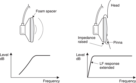
In Figure 5.46 a supra-aural headphone (one which sits above the ear rather than surrounding it) in free space has a very poor LF response because it is a dipole source and at low frequency air simply moves from front to back in a short circuit. However, the presence of the listener’s head obstructs the short circuit and the bass tip-up effect gives a beneficial extension of frequency response to the intended listener, whilst those not wearing the headphones only hear high frequencies. Many personal stereo players incorporate an LF boost to further equalize the losses. All practical headphones must be designed to take account of the presence of the user’s head since headphones work primarily in the near field.
A dramatic example of bass tip-up is obtained by bringing the ear close to the edge of a cymbal shortly after it has been struck. The fundamental note which may only be a few tens of Hz can clearly be heard. As the cymbal is such a poor radiator at this frequency there is very little damping of the fundamental which will continue for some time. At normal distances it is quite inaudible.
If sound enters a medium in which the speed is different, the wavelength will change causing the wavefront to leave the interface at a different angle. This is known as refraction. The ratio of velocity in air to velocity in the medium is known as the refractive index of that medium; it determines the relationship between the angles of the incident and refracted wavefronts. This doesn’t happen much in real life, it requires a thin membrane with different gases each side to demonstrate the effect. However, as was shown above in connection with the Doppler effect, wind has the ability to change the wavelength of sound. Figure 5.47 shows that when there is a wind blowing, friction with the earth’s surface causes a velocity gradient. Sound radiated upwind will have its wavelength shortened more away from the ground than near it, whereas the reverse occurs downwind.
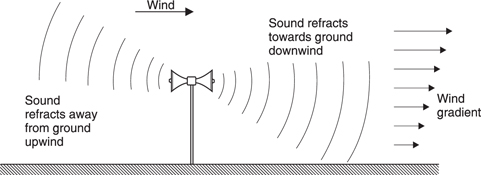
Figure 5.47 When there is a wind, the velocity gradient refracts sound downwards downwind of the source and upwards upwind of the source.
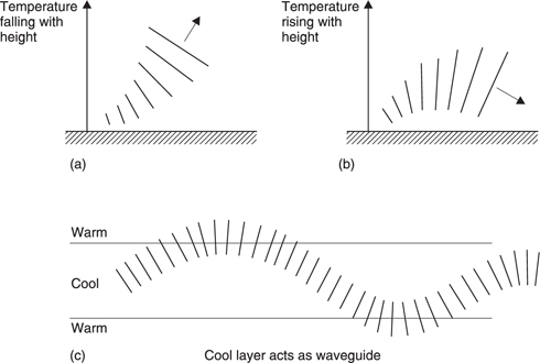
Upwind it is difficult to hear a sound source because the radiation has been refracted upwards whereas downwind the radiation will be refracted towards the ground making the sound ‘carry’ better. Temperature gradients can have the same effect. As Figure 5.48(a) shows, the reduction in the speed of sound due to the normal fall in temperature with altitude acts to refract sound away from the earth. In the case of a temperature inversion (b) the opposite effect happens. Sometimes a layer of air forms in the atmosphere which is cooler than the air above and below it. Figure 5.48(c) shows that this acts as a waveguide because sound attempting to leave the layer is gently curved back in giving the acoustic equivalent of a mirage. In this way sound can travel hundreds of kilometres. Sometimes what appears to be thunder is heard on a clear sunny day. In fact it is the sound from a supersonic aircraft which may be a very long way away indeed.
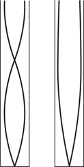
When two sounds of equal frequency and amplitude are travelling in opposite directions, the result is a standing wave where constructive interference occurs at fixed points one wavelength apart with nulls between. This effect can often be found between parallel hard walls, where the space will contain a whole number of wavelengths. As Figure 5.49 shows, a variety of different frequencies can excite standing waves at a given spacing. Wind instruments work on the principle of standing waves. The wind produces broadband noise, and the instrument resonates at the fundamental depending on the length of the pipe. The higher harmonics add to the richness or timbre of the sound produced.
In practice, many real materials do not reflect sound perfectly. As Figure 5.50 shows, some sound is reflected, some is transmitted and the remainder is absorbed. The proportions of each will generally vary with frequency. Only porous materials are capable of being effective sound absorbers. The air movement is slowed by viscous friction among the fibres. Such materials include wood, foam, cloth and carpet. Non-porous materials either reflect or transmit according to their mass. Thin, hard materials such as glass, reflect high frequencies but transmit low frequencies. Substantial mass is required to prevent transmission of low frequencies, there being no substitute for masonry.
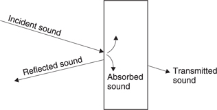
Figure 5.50 Incident sound is partially reflected, partially transmitted and partially absorbed. The proportions vary from one material to another and with frequency.
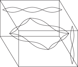
In real rooms with hard walls, standing waves can be set up in many dimensions, as Figure 5.51 shows. The frequencies at which the dominant standing waves occur are called eigentones. Any sound produced in such a room which coincides in frequency with an eigentone will be strongly emphasized as a resonance which might take some time to decay. Clearly a cube would be the worst possible shape for a studio as it would have a small number of very powerful resonances.
At the opposite extreme, an anechoic chamber is a room treated with efficent absorption on every surface. Figure 5.52 shows that long wedges of foam absorb sound by repeated reflection and absorption down to a frequency determined by the length of the wedges (our friend ka again). Some people become distressed in anechoic rooms and musical instruments sound quiet, lifeless and boring. Sound of this kind is described as dry.
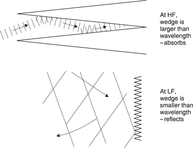
Figure 5.52 Anechoic wedges are effective until wavelength becomes too large to see them.
Reflected sound is needed in concert halls to amplify the instruments and add richness or reverberation to the sound. Since reflection cannot and should not be eliminated, practical studios, listening rooms and concert halls are designed so that resonances are made as numerous and close together as possible so that no single one appears dominant. Apart from choosing an irregular shape, this goal can be helped by the use of diffusers which are highly irregular reflectors. Figure 5.53 shows that if a two-plane stepped surface is made from a reflecting material, at some wavelengths there will be destructive interference between sound reflected from the upper surface and sound reflected from the lower. Consequently the sound cannot reflect back the way it came but must diffract off at any angle where constructive interference can occur. A diffuser made with steps of various dimensions will reflect sound in a complex manner. Diffusers are thus very good at preventing standing waves without the deadening effect that absorbing the sound would have.
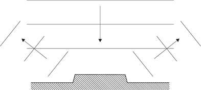
Figure 5.53 A diffuser prevents simple reflection of an incident wavefront by destructive interference. The diffracted sound must leave by another path.
In a hall having highly reflective walls, any sound will continue to reflect around for some time after the source has ceased. Clearly as more absorbent is introduced, this time will fall. The time taken for the sound to decay by 60 dB is known as the reverberation time of the room. The optimum reverberation time depends upon the kind of use to which the hall is put. Long reverberation times make orchestral music sound rich and full, but would result in intelligibility loss on speech. Consequently theatres and cinemas have short reverberation times, opera houses have medium times and concert halls have the longest. In some multi-purpose halls the reverberation can be modified by rotating wall panelling, although more recently this is done with electronic artificial reverberation using microphones, signal processors and loudspeakers.
Only porous materials make effective absorbers at high frequency, but these cannot be used in areas which are prone to dampness or where frequent cleaning is required. This is why indoor swimming pools are so noisy.
5.11 Directionality in hearing
An understanding of the mechanisms of direction sensing is important for the successful implementation of spatial illusions such as stereophonic and surround sound. The nerve impulses from the ears are processed in specific areas of the brain which appear to have evolved at different times to provide different types of information. The time-domain response works quickly, primarily aiding the direction-sensing mechanism, and is older in evolutionary terms. The frequency-domain response works more slowly, aiding the determination of pitch and timbre and developed later, presumably after speech evolved.
The earliest use of hearing was as a survival mechanism to augment vision. The most important aspect of the hearing mechanism was the ability to determine the location of the sound source. Figure 5.54 shows that the brain can examine several possible differences between the signals reaching the two ears. At (a) a phase shift will be apparent. At (b) the distant ear is shaded by the head resulting in a different frequency response compared to the nearer ear. At (c) a transient sound arrives later at the more distant ear. The inter-aural phase, delay and level mechanisms vary in their effectiveness depending on the nature of the sound to be located. At some point a fuzzy logic decision has to be made as to how the information from these different mechanisms will be weighted.
There will be considerable variation with frequency in the phase shift between the ears. At a low frequency such as 30 Hz, the wavelength is around 11.5 metres and so this mechanism must be quite weak at low frequencies. At high frequencies the ear spacing is many wavelengths producing a confusing and complex phase relationship. This suggests a frequency limit of around 1500 Hz which has been confirmed by experiment.
At low and middle frequencies sound will diffract round the head sufficiently well that there will be no significant difference between the level at the two ears. Only at high frequencies does sound become directional enough for the head to shade the distant ear causing what is called an inter-aural intensity difference (IID).
Phase differences are only useful at low frequencies and shading only works at high frequencies. Fortunately real-world sounds are timbral or broadband and often contain transients. Timbral, broadband and transient sounds differ from tones in that they contain many different frequencies.
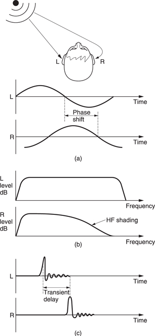
A transient has an unique aperiodic waveform which, as Figure 5.54(c) shows, suffers no ambiguity in the assessment of inter-aural delay (IAD) between two versions. Note that a 1° change in sound location causes an IAD of around 10 microseconds. The smallest detectable IAD is a remarkable 6 microseconds. This should be the criterion for spatial reproduction accuracy.
A timbral waveform is periodic at the fundamental frequency but the presence of harmonics means that a greater number of nerve firings can be compared between the two ears. As the statistical deviation of nerve firings with respect to the incoming waveform is about 100 microseconds the only way in which an IAD of 6 microseconds can be resolved is if the timing of many nerve firings is correlated in some way in the brain.
Transient noises produce a one-off pressure step whose source is accurately and instinctively located. Figure 5.55 shows an idealized transient pressure waveform following an acoustic event. Only the initial transient pressure change is required for location. The time of arrival of the transient at the two ears will be different and will locate the source laterally within a processing delay of around a millisecond.
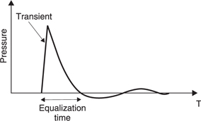
Figure 5.55 Following an acoustic event, a pressure step is created, but this cannot be sustained by the surrounding air and rapidly decays. The time of arrival difference of the transient at the two ears allows direction to be discerned and the time taken for the pressure to equalize allows the size of the source to be estimated.
Following the event which generated the transient, the air pressure equalizes. The time taken for this equalization varies and allows the listener to establish the likely size of the sound source. The larger the source, the longer the pressure-equalization time. Only after this does the frequency analysis mechanism tell anything about the pitch and timbre of the sound.
The above results suggest that anything in a sound reproduction system which impairs the reproduction of a transient pressure change will damage localization and the assessment of the pressure-equalization time. Clearly in an audio system which claims to offer any degree of precision, every component must be able to reproduce transients accurately and must have at least a minimum phase characteristic if it cannot be phase-linear. In this respect digital audio represents a distinct technical performance advantage although much of this is lost in poor transducer design, especially in loudspeakers.
It must be appreciated that the HAS can locate a number of different sound sources simultaneously. The HAS must constantly be comparing excitation patterns from the two ears with different delays. Strong correlation will be found where the delay corresponds to the interaural delay for a given source. This is apparent in the binaural threshold of hearing which is 3–6 dB better than monaural at around 4 kHz. This delay-varying mechanism will take time and it is to be expected that the HAS would then be slow to react to changes in source direction. This is indeed the case and experiments have shown that oscillating sources can only be tracked up to 2–3 Hz.8 The ability to locate bursts of noise improves with burst duration up to about 700 milliseconds.
The perception we have of when a sound stops and starts is not very precise. This is just as well because we live in a reverberant world which is filled with sound reflections. If we could separately distinguish every different reflection in a reverberant room we would hear a confusing cacaphony. In practice we hear very well in reverberant surroundings, far better than microphones can, because of the transform nature of the ear and the way in which the brain processes nerve signals.
When two or more versions of a sound arrive at the ear, provided they fall within a time span of about 30 ms, they will not be treated as separate sounds, but will be fused into one sound. Only when the time separation reaches 50–60 ms do the delayed sounds appear as echoes from different directions. As we have evolved to function in reverberant surroundings, reflections do not impair our ability to locate the source of a sound. The fusion will be impaired if the spectra of the two sounds are too dissimilar.
A moment’s thought will confirm that the first version of a transient sound to reach the ears must be the one which has travelled by the shortest path. Clearly this must be the direct sound rather than a reflection. Consequently the HAS has evolved to attribute source direction from the time of arrival difference at the two ears of the first version of a transient. Later versions which may arrive from elsewhere simply add to the perceived loudness but do not change the perceived location of the source.
This phenomenon is known as the precedence or Haas effect after the Dutch researcher who investigated it. Haas found that the precedence effect is so powerful that even when later-arriving sounds are artificially amplified (a situation which does not occur in nature) the location still appears to be that from which the first version arrives. Figure 5.56 shows how much extra level is needed to overcome the precedence effect as a function of arrival delay.
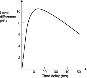
Experiments have been conducted in which the delay and intensity clues are contradictory to investigate the way the weighting process works. The same sound is produced in two locations but with varying relative delay and shading-dependent level. The way in which the listener perceives an apparent sound direction reveals how the directional clues are weighted.
Within the maximum inter-aural delay of about 700 microseconds the precedence effect does not function and the perceived direction can be pulled away from that of the first-arriving source by an increase in level. Figure 5.57 shows that this area is known as the time–intensity trading region. Once the maximum inter-aural delay is exceeded, the HAS knows that the time difference must be due to reverberation and the trading ceases to change with level.
It is important to realize that in real life the HAS expects a familiar sound to have a familiar weighting of phase, time of arrival and shading clues. A high-quality sound reproduction system must do the same if a convincing spatial illusion is to be had. Consequently a stereo or surround system which attempts to rely on just one of these effects will not sound realistic. Worse still is a system which relies on one effect to be dominant but where another is contradictory.
In the presence of an array of simultaneous sound sources the HAS has an ability to concentrate on one of them based on its direction. The brain appears to be able to insert a controllable time delay in the nerve signals from one ear with respect to the other so that when sound arrives from a given direction the nerve signals from both ears are coherent. Sounds arriving from other directions are incoherent and are heard less well. This is known as attentional selectivity9 but is more usually referred to as the cocktail party effect.
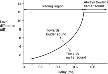
Monophonic systems prevent the use of this effect completely because the first version of all sounds reaching the listener come from the same loudspeaker. Stereophonic systems allow the cocktail party effect to function in that the listener can concentrate on specific sound sources in a reproduced stereophonic image with the same facility as in the original sound.
One of the most compelling demonstrations of stereo is to make a stereophonic recording of a crowded function in a reverberant room. On replaying several times it will be possible to attentional selectivity to listen to a different conversation each time. Upon switching to mono it will be found that the result is completely unintelligible. A corollary of this experiment is that if this result is not obtained, there is a defect in the equipment or the hearing of the listener.
One of the most frustrating aspects of hearing impairment is that hearing loss in one ear destroys the ability to use the cocktail party effect. In quiet surroundings many people with hearing loss can follow what is said in normal tones. In a crowded room they are at a serious disadvantage because they cannot select a preferred sound source.
Laterally separated ears are ideal for determining the location of sound sources in the plane of the earth’s surface, which is after all where most sound sources emanate. In comparison our ability to determine height in sound is very poor. As the ears are almost exactly half-way back on each side of the head it is quite possible for sound sources ahead or behind, above or below to produce almost the same relative delay, phase shift and shading resulting in an ambiguity. This leads to the concept of the cone of confusion where all sources on a cone with the listener at the vertex will result in the same IAD.
There are two main ways in which the ambiguity can be resolved. If a plausible source of sound can be seen, then the visual clue will dominate. Experience will also be used. People who look up when they hear birdsong may not be able to determine the height of the source at all, they may simply know, as we all do, that birds sing in trees.
A second way of resolving front/back ambiguity is to turn the head slightly. This is often done involuntarily and most people are not aware they are using the technique. In fact when people deliberately try harder to locate a sound they often keep their head quite still making the ambiguity worse. Section 5.14 will show why intensity stereo recordings are fundamentally incompatible with headphone reproduction. A further problem with headphones is that they turn with the wearer’s head, disabling the ability to resolve direction by that means.
The convolutions of the pinna also have some effect at high frequencies where the wavelength of sound is sufficiently short. The pinna produces a comb-filtering spectral modification which is direction dependent. Figure 5.58 shows that different parts of the pinna cause reflections according to the direction from which the sound has come. The different reflection mechanisms result in notches or cancellations at various frequencies. The hearing mechanism learns the position of these notches in order to make height judgements with suitable types of sound source.
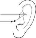
Figure 5.58 The pinna plays a part in determining direction at high frequencies where reflections cause recognizable notches in the spectrum which are a function of geometry.
Figure 5.59 shows that when standing, sounds from above reach the ear directly and via a ground reflection which has come via a longer path. (There is also a smaller effect due to reflection from the shoulders). At certain frequencies the extra path length will correspond to a 180° phase shift, causing cancellation at the ear. The result is a frequency response consisting of evenly spaced nulls which is called comb filtering. A moving object such as a plane flying over will suffer changing geometry which will cause the frequency of the nulls to fall towards the point where the overhead position is reached.
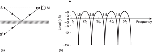
Figure 5.59 Comb-filtering effect produced by interference between a sound wave and a delayed version of itself. (a) Microphone M receives direct wave from source S and a delayed wave from image sound source S1. (b) Frequency response shows alternating peaks and troughs resembling the teeth of a comb.
The direction-sensing ability has been examined by making binaural recordings using miniature microphones actually placed down the ear canals of a volunteer. When these are played back on headphones to the person whose ears were used for the recording, full localization of direction including front/rear and height discrimination is obtained. However, the differences between people’s ears are such that the results of playing the recording to someone else are much worse. The same result is obtained if a dummy head is used.
Whilst binaural recordings give very realistic spatial effects, these effects are only obtained on headphones and consequently the technique is unsatisfactory for signals intended for loudspeaker reproduction and cannot be used in prerecorded music, radio or television.
When considering the localization ability of sound, it should be appreciated that vision can produce a very strong clue. If only one person can be seen speaking in a crowd, then any speech heard must be coming from that person. The same is true when watching films or television. This is a bonus because it means that the utmost precision is not required in the spatial accuracy of stereo or surround sound accompanying pictures. However, if the inaccuracy is too great fatigue may result and the viewer may have a displacement of localization for some time afterwards.10
5.12 Microphone principles
Digital techniques are popular in audio because they allow ease of processing, storage and transmission with great precision. In order to enter the digital domain it is essential to have transducers such as microphones and loudspeakers which can convert between real sound and an electrical equivalent. Figure 5.60(a) shows that even if the convertors and the digital system are ideal, the overall quality of a sound system is limited by the quality of both microphone and loudspeaker. In a broadcast sound system or when selling prerecorded material on media or over a network, the quality of the final loudspeaker is variable, dependent upon what the consumer can afford as shown in (b).
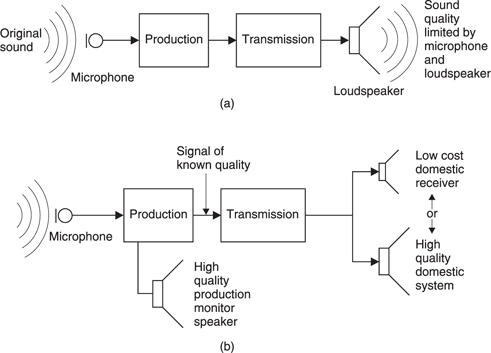
However, it must be assumed that at least a number of consumers will have high-quality systems. The quality of the sound should exceed or at least equal that of the consumer’s equipment even after all the recording, production and distribution processes have been carried out. Consequently the microphone used in production must be of high quality. The microphone is a measuring device and its output consists of information rather than power. It is possible to conceive of an ideal microphone and the best practice approaches this quite closely. The loudspeakers used for monitoring the production process must also be of high quality so that any defect in the microphone or elsewhere can be identified. However, loudspeakers have to transduce power, not just information and this is harder.
The job of the microphone is to convert sound into an electrical signal. Sound consists of both pressure and velocity variations and microphones can use either or both in order to obtain various directional characteristics.11 The polar or directional characteristics of a microphone are most important and are treated here before consideration of the operating principle. Polar characteristics assume even greater importance if the illusion of stereophony is to be made realistic.
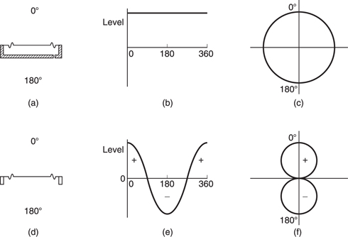
Figure 5.61 (a) Pressure microphone only allows sound to reach one side of the diaphragm. (b) Pressure microphone is omnidirectional for small ka. (c) Directional characteristic is more intuitive when displayed in polar form. (d) Velocity or pressure gradient microphone exposes both sides of diaphragm. (e) Output of velocity microphone is a sinusoidal function of direction. (f) In polar coordinates velocity microphone shows characteristic figure-of-eight shape for small ka.
Figure 5.61(a) shows a true pressure microphone which consists of a diaphragm stretched across an otherwise sealed chamber. In practice a small pinhole is provided to allow changes in atmospheric pressure to take place without causing damage. Some means is provided to sense the diaphragm motion and convert it into an electrical output signal. This can be done in several ways which will be considered below. The output of such a microphone for small values of ka is completely independent of direction as (b) shows.
Unlike the HAS, which is selective, microphones reproduce every sound which reaches them. Figure 5.62(a) shows the result of placing a microphone near to a hard wall. The microphone receives a combination of direct and reflected sound between which there is a path length difference. At frequencies where this amounts to a multiple of a wavelength, the reflection will reinforce the direct sound, but at intermediate frequencies cancellation will occur, giving a comb filtering effect. Clearly a conventional microphone should not be positioned near a reflecting object.
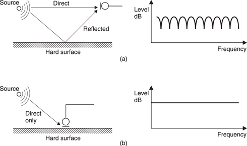
The path length difference is zero at the wall itself. The pressure zone microphone (PZM) of Figure 5.62(b) is designed to be placed on flat surfaces where it will not suffer from reflections. A pressure capsule is placed facing and parallel to a flat surface at a distance which is small compared to the shortest wavelength of interest. The acoustic impedance rises at a boundary because only a half-space can be seen and the output of a PZM is beneficially doubled.
Figure 5.61(d) shows the pressure gradient microphone in which the diaphragm is suspended in free air from a symmetrical perimeter frame. The maximum excursion of the diaphragm will occur when it faces squarely across the incident sound. As (e) shows, the output will fall as the sound moves away from this axis, reaching a null at 90°. If the diaphragm were truly weightless then it would follow the variations in air velocity perfectly, hence the term velocity microphone. However as the diaphragm has finite mass then a pressure difference is required to make it move, hence the more accurate term pressure gradient microphone.
The pressure gradient microphone works by sampling the passing sound wave at two places separated by the front-to-back distance. Figure 5.63 shows that the pressure difference rises with frequency as the frontto- back distance becomes a greater part of the cycle. The force on the diaphragm rises at 6 dB/octave. Eventually the distance exceeds half the wavelength at the critical frequency where the pressure gradient effect falls rapidly. Fortunately the rear of the diaphragm will be starting to experience shading at this frequency so that the drive is only from the front. This has the beneficial effect of transferring to pressure operation so that the loss of output is not as severe as the figure suggests. The pressure gradient signal is in phase with the particle displacement and is in quadrature with the particle velocity.
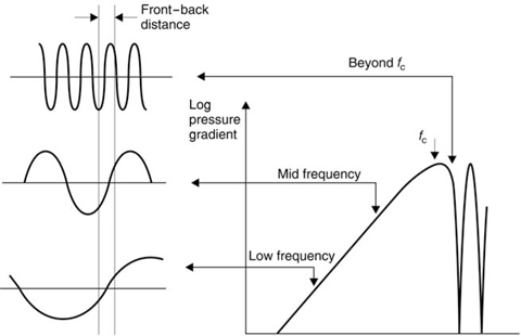
In practice the directional characteristics shown in Figure 5.61(b) and (e) are redrawn in polar coordinates such that the magnitude of the response of the microphone corresponds to the distance from the centre point at any angle. The pressure microphone (c) has a circular polar diagram as it is omnidirectional or omni for short. Omni microphones are good at picking up ambience and reverberation which makes them attractive for music and sound effects recordings in good locations. In acoustically poor locations they cannot be used because they are unable to discriminate between wanted and unwanted sound. Directional microphones are used instead.
The PG microphone has a polar diagram (f) which is the shape of a figure-of-eight. Note the null at 90° and that the polarity of the output reverses beyond 90° giving rise to the term dipole. The figure-of-eight microphone (sometimes just called ‘an eight’) responds in two directions giving a degree of ambience pickup, although the sound will be a little drier than that of an omni. A great advantage of the figure-of-eight microphone over the omni is that it can reject an unwanted sound. Rather than point the microphone at the wanted sound, a better result will be obtained by pointing the null or dip in the polar diagram at the source of the unwanted sound.
Unfortunately the pressure gradient microphone cannot distinguish between gradients due to sound and those due to gusts of wind. Consequently PG microphones are more sensitive to wind noise than omnis.
If an omni and an eight are mounted coincidentally, various useful results can be obtained by combining the outputs. Figure 5.64(a) shows that if the omni and eight signals are added equally, the result is a heartshaped polar diagram called a cardioid. This response is obtained because at the back of the eight the output is antiphase and has to be subtracted from the output of the omni. With equal signals this results in a null at the rear and a doubling at the front. This useful polar response will naturally sound drier than an eight, but will have the advantage of rejecting more unwanted sound under poor conditions. In public address applications, use of a cardioid will help to prevent feedback or howl-round which occurs when the microphone picks up too much of the signal from the loudspeakers. Virtually all hand-held microphones have a cardioid response where the major lobe faces axially so that the microphone is pointed at the sound source. This is known as an end-fire configuration shown in Figure 5.64(b).
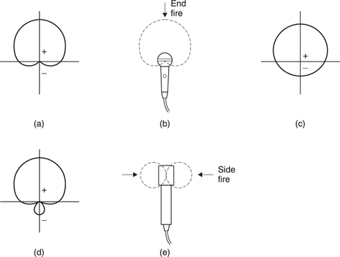
Figure 5.64 (a) Combining an omni response with that of an eight in equal amounts produces the useful cardioid directivity pattern. (b) Hand-held fixed cardioid response microphones are usually built in the end-fire configuration where the body is placed in the null. (c) Sub-cardioid obtained by having more omni in the mix gives better ambience pickup than cardioid. (d) Hyper-cardioid obtained by having more eight in the mix is more directional than cardioid but the presence of the rear lobe must be considered in practice. (e) Microphones with variable polar diagram are generally built in the side-fire configuration.
Where a fixed cardioid-only response is required, this can be obtained using a single diaphragm where the chamber behind it is not sealed, but open to the air via an acoustic labyrinth. Figure 5.65(a) shows that the asymmetry of the labyrinth means that sound which is incident from the front reaches the rear of the diaphragm after a path difference allowing pressure gradient operation. Sound from the rear arrives at both sides of the diaphragm simultaneously, nulling the pressure gradient effect. Sound incident at 90° experiences half the path length difference, giving a reduced output in comparison with the on-axis case. The overall response has a cardioid polar diagram. This approach is almost universal in hand-held cardioid microphones.
In variable directivity microphones there are two such cardioid mechanisms facing in opposite directions as shown in Figure 5.65(b). The system was first devised by the Neumann Company.12 The central baffle block contains a pattern of tiny holes, some of which are drilled right through and some of which are blind. The blind holes increase the volume behind the diaphragms, reducing the resonant frequency in pressure operation when the diaphragms move in anti-phase. The holes add damping because the viscosity of air is significant in such small cross-sections.
The through-drilled holes allow the two diaphragms to move in tandem so that pressure gradient operation is allowed along with further damping. Figure 5.65(c) shows that sound incident from one side acts on the outside of the diaphragm on that side directly, but passes through the other diaphragm and then through the cross-drilled holes to act on the inside of the first diaphragm. The path length difference creates the pressure gradient condition. Sound from the ‘wrong’ side (d) arrives at both sides of the far diaphragm without a path length difference.
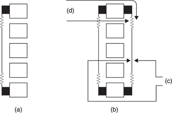
Figure 5.65 (a) Fixed cardioid response is obtained with a labyrinth delaying sound reaching the rear of the diaphragm. (b) Double cardioid capsule is the basis of the variable directivity microphone. (c) Sound arriving from the same side experiences a path-length difference to create a pressure gradient. (d) Sound arriving from the opposite side sees no path-length difference and fails to excite diaphragm.
The relative polarity and amplitude of signals from the two diaphragms can be varied by a control. By disabling one or other signal, a cardioid response can be obtained. Combining them equally results in an omni, whereas combining them with an inversion results in a figure-ofeight response. Unequal combination can obtain the sub-cardioid shown in Figure 5.64(c) or a hyper-cardioid shown in Figure 5.64(d).
Where a flexible polar response is required, the end-fire configuration cannot be used as the microphone body would then block the rearward access to the diaphragm. The side-fire configuration is shown in Figure 5.64(e) where the microphone is positioned across the approaching sound, usually in a vertical position. For picture applications where the microphone has to be out of shot such microphones are often slung from above pointing vertically downwards.
In most applications the polar diagrams noted above are adequate, but on occasions it proves to be quite impossible to approach the subject close enough and then a highly directional microphone is needed. Picking up ball sounds in sport is one application. Figure 5.66(a) shows that the shotgun microphone consists of a conventional microphone capsule which is mounted at one end of a slotted tube. Sound wavefronts approaching from an angle will be diffracted by the slots such that each slot becomes a reradiator launching sound down the inside of the tube. However, Figure 5.66(b) shows that the radiation from the slots travelling down the tube will not add coherently and will be largely cancelled. A wavefront approaching directly on axis as in (c) will pass directly down the outside and the inside of the tube as if the tube were not there and consequently will give a maximum output.
The directivity patterns shown here are only obtained where ka is small and are thus ideal. In practice at high frequencies ka will not be small and the actual polar diagram will differ due to diffraction becoming significant.
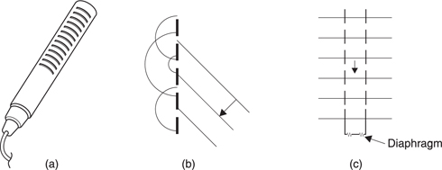
Figure 5.66 (a) Shotgun microphone has slotted tube. (b) Off-axis sound enters slots to produce multiple incoherent sources which cancel. (c) On-axis sound is unaware of tube.
Figure 5.67(a) shows the result of a high-frequency sound arriving offaxis at a large diaphragm. It will be clear that at different parts of the diaphragm the sound has a different phase and that in an extreme case cancellation will occur, reducing the output significantly.
When the sound is even further off-axis, shading will occur. Consequently at high frequency the polar diagram of a nominally omni microphone may look something like that shown in Figure 5.67(b). The HF polar diagram of an eight may resemble (c). Note the narrowing of the response such that proper reproduction of high frequencies is only achieved when the source is close to the axis.
The frequency response of a microphone should ideally be flat and this is often tested on-axis in anechoic conditions. However, in practical use the surroundings will often be reverberant and this will change the response at high frequencies because the directivity is not independent of frequency. Consequently a microphone which is flat on-axis but which has a directivity pattern which narrows with frequency will sound dull in practical use. Conversely a microphone which has been equalized flat in reverberant surroundings may appear too bright to an on-axis source.
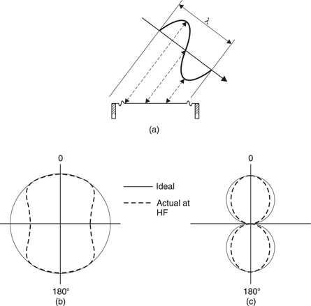
Figure 5.67 (a) Off-axis response is impaired when ka is not small because the wavefront reaches different parts of diaphragm at different times causing an aperture effect. (b) Polar diagram of practical omni microphone at high frequency shows narrowing of frontal response due to aperture effect and rear loss due to shading. (c) Practical eight microphone has narrowing response at high frequency.
Pressure microphones being omnidirectional have the most difficulty in this respect because shading makes it almost impossible to maintain the omnidirectional response at high frequencies. Clearly an omni based on two opposing cardioids will be better at high frequencies than a singlepressure capsule. Another possibility is to mount the diaphragm horizontally and place a conical reflector above it.
It is possible to reduce ka by making the microphone diaphragm smaller but this results in smaller signals making low noise difficult to achieve. However, developments in low-noise circuitry will allow diaphragm size beneficially to be reduced.
In the case of the shotgun microphone, the tube will become acoustically small at low frequencies and will become ineffective causing the polar diagram to widen.
The electrical output from a microphone can suffer from distortion with very loud signals or from noise with very quiet signals. In passive microphones distortion will be due to the linear travel of the diaphragm being exceeded whereas in active microphones there is the additional possibility of the circuitry being unable to handle large-amplitude signals. Generally a maximum SPL will be quoted at which a microphone produces more than 0.5 per cent THD.
Noise will be due to thermal effects in the transducer itself and in the circuitry. Microphone noise is generally quoted as the SPL which would produce the same level as the noise. The figure is usually derived for the noise after A weighting (see section 5.5). The difference between the 0.5 per cent distortion SPL and the self-noise SPL is the dynamic range of the microphone: 110 dB is considered good but some units reach an exceptional 130 dB.
In addition to thermal noise, microphones may also pick up unwanted signals and hum fields from video monitors, lighting dimmers and radio transmissions. Considering the low signal levels involved, microphones have to be well designed to reject this kind of interference. The use of metal bodies and grilles is common to provide good RF screening.
The output voltage for a given SPL is called the sensitivity. The specification of sensitivity is subject to as much variation as the mounting screw thread. Some data sheets quote output voltage for 1 Pa, some for 0.1 Pa. Sometimes the output level is quoted in dBV, sometimes dBu (see section 5.2). The outcome is that in practice preamplifier manufacturers provide a phenomenal range of gain on microphone inputs and the user simply turns up the gain to get a reasonable level.
It should be noted that in reverberant conditions pressure and pressure gradient microphones can give widely differing results. For example, where standing waves are encountered, a pressure microphone positioned at a pressure node would give an increased output whereas a pressure gradient microphone in the same place would give a reduced output. The effect plays havoc with the polar diagram of a cardioid microphone.
The proximity effect should always be considered when placing microphones. As explained above, proximity effect causes an emphasis of low frequencies when a PG microphone is too close to a source. A true PG microphone such as an eight will suffer the most, whereas a cardioid will have 6 dB less proximity effect because half of the signal comes from an omni response.
5.13 Microphone mechanisms
There are two basic mechanisms upon which microphone operation is based: electrostatic and electrodynamic. The electrodynamic microphone operates on the principle that a conductor moving through a magnetic field will generate a voltage proportional to the rate of change of flux. As the magnetic flux is constant, then this results in an output proportional to the velocity of the conductor, i.e. it is a constant velocity transducer. The most common type has a moving coil driven by a diaphragm. In the ribbon microphone the diaphragm itself is the conductor.
The electrostatic microphone works on the variation in capacitance between a moving diaphragm and a fixed plate. As the capacitance varies directly with the spacing the electrostatic microphone is a constant amplitude transducer. There are two forms of electrostatic microphone: the condensor, or capacitor, microphone and the electret microphone.
The ribbon and electrostatic microphones have the advantage that there is extremely direct coupling between the sound waveform and the electrical output and so very high quality can be achieved. The movingcoil microphone is considered to be of lower quality but is cheaper and more robust.
Microphones can be made using other techniques but none can offer high quality and use is restricted to consumer or communications purposes or where something unbreakable is required.
Figure 5.68(a) shows that the vibrations of a diaphragm can alter the pressure on a quantity of carbon granules, altering their resistance to current flow. This construction was used for telephone mouthpieces for many years. Whilst adequate for speech, the noise level and distortion is high.
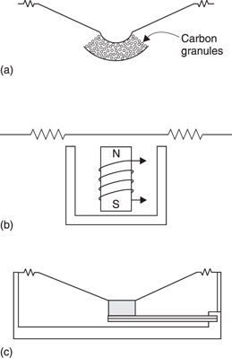
Figure 5.68(b) shows the moving-iron or variable reluctance microphone in which a ferrous diaphragm vibrates adjacent to a permanent magnet. The variation of the air gap causes the flux of the magnet to vary and this induces a signal in a coil.
Figure 5.68(c) shows a piezo-electric or crystal microphone in which the diaphragm vibrations deform a bimorph crystal of Rochelle salt or barium titanate. This material produces a voltage when under strain. A high input impedance is required.
There are two basic implementations of the electrodynamic microphone; the ribbon and the moving coil. Figure 5.69(a) shows that in the ribbon microphone the diaphragm is a very light metallic foil which is suspended under light tension between the poles of a powerful magnet. The incident sound causes the diaphragm to move and the velocity of the motion results in an EMF being generated across the ends of the ribbon.
The most common form which the ribbon microphone takes is the figure-of-eight response although cardioid and pressure variants are possible using the techniques outlined above. The output voltage of the ribbon is very small but the source impedance of the ribbon is also very low and so it is possible to use a transformer to produce a higher output voltage at a more convenient impedance.
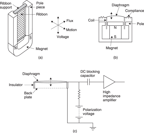
Figure 5.69 (a) Now obsolete ribbon microphone suspends conductive diaphragm in magnetic field. Low output impedance requires matching transformer. (b) The moving-coil microphone is robust but indirect coupling impairs quality. (c) Capacitor microphone has very tight coupling but requires high-impedance electronics and needs to be kept dry.
As the driving force on a pressure gradient transducer is proportional to frequency, the resonant frequency of the ribbon is set below the audio band at only a few Hz. Consequently the ribbon works in the masscontrolled region where for constant drive force the velocity falls at 6 dB/ octave. This balances the 6 dB/octave rise of the pressure gradient effect to produce a flat response. The very high compliance needed to set the resonance below the audio band means that the ribbon microphone is shock sensitive. If the body of the microphone is moved, the diaphragm will lag behind causing relative motion. Good mounting isolation is required.
The advantage of the ribbon microphone is that the motion of the ribbon is directly converted to an electrical signal. This is potentially very accurate. However, unless the transformer is of extremely high quality the inherent accuracy will be lost. A further problem is that to obtain reasonable sensitivity the diaphragm must be relatively large, giving a low cut-off frequency and leading to the directivity problems mentioned above. Traditionally the magnet was also large, leading to a heavy construction. A further problem is that the diaphragm is extremely delicate and a single exposure to wind might destroy it.
Although the ribbon microphone was at one time the best available it has been overshadowed by the capacitor microphone and is little used today. The ribbon principle deserves to be revisited with modern techniques. A smaller diaphragm and a physically smaller rare-earth magnet would push up the cut-off frequency by reducing the path length difference. The smaller output could be offset by incorporating an amplifier into an active design.
The most common version of the electrodynamic microphone is the moving-coil system shown in Figure 5.69(b). The diaphragm is connected to a cylindrical former upon which is wound a light coil of wire. The coil operates in the radial flux pattern of a cylindrical magnet. As the output is proportional to velocity, a moving-coil pressure microphone has to work in the resistance-controlled domain using a mid-band resonance which is heavily damped. The range is often extended by building in additional damped resonances. A moving-coil pressure gradient microphone would need to operate in mass-control.
As it is possible to wind many turns of wire on the coil, the output of such a microphone is relatively high. The structure is quite robust and can easily withstand wind and handling abuse. However, the indirect conversion, whereby the sound moves the diaphragm and the diaphragm moves the coil, gives impaired performance because the coil increases the moving mass and the mechanical coupling between the coil and diaphragm is never ideal. Consequently the moving-coil microphone, generally in a cardioid response form, finds common application in outdoor use, for speech or for public address, but is considered inadequate for accurate music work.
In the capacitor (or condensor) microphone the diaphragm is highly insulated from the body of the microphone and is fed with a high polarizing voltage via a large resistance. Figure 5.69(c) shows that a fixed metallic grid forms a capacitor in conjunction with the diaphragm. The diaphragm is connected to an amplifier having a very high impedance. The high impedances mean that there is essentially a constant charge condition. Consequently when incident sound moves the diaphragm and the capacitance between it and the grid varies, the result will be a change of diaphragm voltage which can be amplified to produce an output.
As the condenser mechanism has a constant amplitude characteristic, a pressure or omni condensor microphone needs to use stiffness control to obtain a flat response. The resonant frequency is placed above the audio band. In a PG condensor microphone resistance control has to be used where a well-damped mid-band resonant frequency is employed.
The condensor microphone requires active circuitry close to the capsule and this requires a source of DC power. This is often provided using the same wires as the audio output using the principle of phantom powering.
If the impedance seen by the condensor is not extremely high, charge can leak away when the diaphragm moves. This will result in poor output and phase shift at low frequencies. As the condensor microphone requires high impedances to work properly, it is at a disadvantage in damp conditions which means that in practice it has to be kept indoors in all but the most favourable weather. Some condensor microphones contain a heating element which is designed to drive out moisture. In older designs based on vacuum tubes, the heat from the tube filaments would serve the same purpose. If a capacitor microphone has become damp, it may fail completely or create a great deal of output noise until it has dried out.
In the electret microphone a material is employed which can produce a constant electric field without power. It is the electrostatic equivalent of a permanent magnet. An electret is a extremely good insulator which has been heated in an intense electric field. A conductor moving in such a field will produce a high-impedance output which will usually require to be locally amplified. The electret microphone can be made very light because no magnet is required. This is useful for hand-held and miniature designs.
In early designs the diaphragm itself was the polarized element, but this required an excessively heavy diaphragm. Later designs use a conductive diaphragm like that of a capacitor microphone and the polarized element is part of the backplate. These back-polarized designs usually offer a better frequency response. Whilst phantom power can be used, electret microphones are often powered by a small dry cell incorporated into the microphone body.
In variable directivity condensor microphones the double cardioid principle of Figure 5.65 is often used. However, the variable mixing of the two signals is achieved by changing the polarity and magnitude of the polarizing voltage on one diaphragm such that the diaphragm audio outputs can simply be added. Figure 5.70 shows that one diaphragm is permanently polarized with a positive voltage, whereas the other can be polarized with a range of voltages from positive, through zero, to negative.
When the polarizing voltages are the same, the microphone becomes omni, whereas if they are opposing it becomes an eight. Setting the variable voltage to zero allows the remaining diaphragm to function as a cardioid. A fixed set of patterns may be provided using a switch, or a continuously variable potentiometer may be supplied. Whilst this would appear to be more flexible it has the disadvantage of being less repeatable. It will be clear that this approach cannot be used with the electret microphone which usually has fixed directivity. The pressure zone microphone is an ideal application for the electret principle.
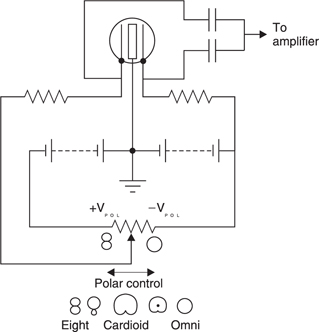
Where active microphones (those containing powered circuitry) are used, it is common to provide the power using the balanced audio cable in reverse. Figure 5.71 shows how phantom powering works. As the audio signal is transmitted differentially, the DC power can be fed to the microphone without interfering with the returning audio signal. The cable screen forms the return path for the DC power.
The use of female XLR connectors for audio inputs is because of phantom power. An audio input is a phantom power output and so requires the insulated contacts of the female connector. Many, but not all, passive microphones are wired such that their differential output is floating relative to the grounded case. These can be used with a cable carrying live phantom power. Provision is generally made to turn the phantom power off so that any type of passive or self-powered microphones can be used.
Variable-directivity microphones may have the directivity control on the microphone body, or they may be provided with a control box which can be some distance away. This can offer practical advantages when a microphone is slung out of reach.
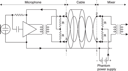
5.14 Stereo and surround sound
The most popular technique for giving an element of spatial realism in sound is stereophony, nowadays abbreviated to stereo, based on two simultaneous audio channels feeding two spaced loudspeakers as shown in Figure 5.72(a). The optimum listening arrangement for stereo is where the speakers and the listener are at different points of a triangle which is almost equilateral.
Delivering more than two channels with analog systems is difficult, but the Dolby Surround system managed to encode rear channel information into two signal channels which were stereo compatible. Further progress in surround sound was made as soon as digital delivery was feasible. In the digital domain any number of channels can be delivered without crosstalk using multiplexing. Figure 5.72(b) shows that in a typical surround installation, five speakers are used, namely Left, Centre, Right, Left rear and Right rear positioned as shown. It is usually beneficial if the rear speakers are mounted somewhat further apart than the front speakers. It is also possible to include a narrow-band signal which drives a monophonic subwoofer. This configuration is known as a 5.1 channel system.
Surround sound works on exactly the same principles as stereo and is no more than an extension of stereo. The principles of stereo will be described here first, before expanding into surround sound.
Stereophony works by creating differences of phase and time of arrival of sound at the listener’s ears. It was shown above that these are the most powerful hearing mechanisms for determining direction. Figure 5.73(a) shows that this time of arrival difference is achieved by producing the same waveform at each speaker simultaneously, but with a difference in the relative level, rather than phase. Each ear picks up sound from both loudspeakers and sums the waveforms.
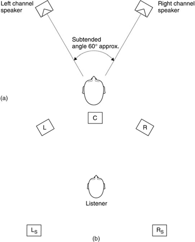
The sound picked up by the ear on the same side as the speaker is in advance of the same sound picked up by the opposite ear. When the level emitted by the left loudspeaker is greater than that emitted by the right, it will be seen from Figure 5.73(b) that the sum of the signals received at the left ear is a waveform which is phase advanced with respect to the sum of the waveforms received at the right ear. If the waveforms concerned are transient the result will be a time of arrival difference. These differences are interpreted as being due to a sound source left of centre.
The stereophonic illusion only works properly if the two loudspeakers are producing in-phase signals. In the case of an accidental phase reversal, the spatial characteristic will be ill-defined and lack images. At low frequencies the two loudspeakers are in one another’s near field and so antiphase connection results in bass cancellation. The same result will be obtained in a surround system if the phase of one or more channels differs from the rest.
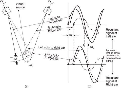
Figure 5.73 (a) Stereo illusion is obtained by producing the same waveform at both speakers, but with different amplitudes. (b) As both ears hear both speakers but at different times, relative level causes apparent time shift at the listener. ΔtL = inter-aural delay due to loudspeaker; ΔtV = inter-aural delay due to virtual source.
As the apparent position of a sound source between the two speakers can be controlled solely by the relative level of the sound emitted by each one, stereo signals in this format are called intensity stereo. In intensity stereo it is possible to ‘steer’ a monophonic signal from a single microphone into a particular position in a stereo image using a form of differential gain control. Figure 5.74 shows that this device, known as a panoramic potentiometer or pan-pot for short, will produce equal outputs when the control is set to the centre. If the pan-pot is moved left or right, one output will increase and the other will reduce, moving or panning the stereo image to one side.
If the system is perfectly linear, more than one sound source can be panned into a stereo image, with each source heard in a different location. This is done using a stereo mixer, shown in Figure 5.75 in which monophonic inputs pass via pan-pots to a stereo mix bus. The majority of pop records are made in this way, usually with the help of a multi-channel recorder with one track per microphone so that mixing and panning can be done at leisure. At one time these recorders were based on analog tape, but today the use of disk drives is becoming universal.
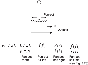
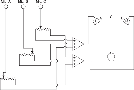
Figure 5.75 Multi-channel mixing technique pans multiple sound sources into one stereo image.
Figure 5.76(a) shows that Dolby Surround derives four channels, L, Centre, R and a surround channel which can be reproduced from two or more rear speakers. In fact a similar speaker arrangement to five-channel discrete can be used. Figure 5.76(b) shows a Dolby Surround encoder. The centre channel is attenuated 3 dB and added equally to L and R. The surround signal is attenuated 3 dB and band limited prior to being encoded with a modified Dolby-B process. The resultant signal is then phase shifted so that a 180° phase relationship is formed between the components which are added to the Lt and Rt signals.
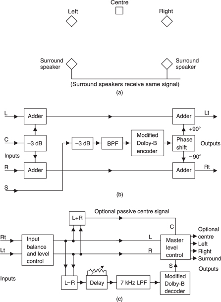
Figure 5.76 (a) Dolby surround sound speaker layout. (b) Dolby surround encoder; see text. (c) Simple passive decoder.
In a simple passive decoder (c) Lt and Rt are used to drive L and R speakers directly. In the absence of a C speaker, the L and R speakers will reproduce the C signal centrally. The added antiphase surround signal will fail to produce an image. If a C speaker is provided, adding Lt and Rt will produce a suitable signal to drive it, although this will result in narrowing of the frontal image. Subtracting Lt and Rt will result in sum of the surround signal and any difference between the original L, R signals. This is band limited then passed through the Dolby-B decoder to produce a surround output.
The Dolby-B-like processing is designed to reduce audibility of L minus R breakthrough on the S signal, particularly on sibilants. The degree of compression is less than that in true Dolby-B to prevent difficulties when Lt and Rt are used as direct speaker drive signals.
In the Pro-logic decoder, shown in Figure 5.76(d) the sum and difference stages are replaced with variable matrices which can act like a two-dimensional pan-pot or steering system. A simple decoder performs poorly when a single point source of sound is present in quiet surroundings whereas a steered decoder will reduce the crosstalk output from unwanted channels. The steering is done by analysing the input signals to identify dominant sound sources. Figure 5.76(d) shows that comparison of the Lt and Rt signals will extract left/right dominance, whereas comparison of sum and difference signals will extract front/rear dominance.
Given that a sound source can be panned between a pair of speakers in front of the listener, with a slight increase in complexity a sound source can be panned between Left, Centre and Right speakers. Figure 5.77 shows that this is done by treating Left and Centre as one stereo pair and Centre and Right as another. A virtual sound source can be positioned anywhere between the Left and Centre speakers by controlling the relative level whilst the Right speaker remains silent. When the sound source is panned completely to the Centre speaker, further movement to the right is possible by feeding some signal to the Right speaker whilst the Left speaker remains silent.
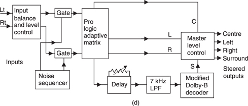
Figure 5.76 (d) (d) Pro-logic decoder uses variable matrices driven by analysis of dominant sound source location.
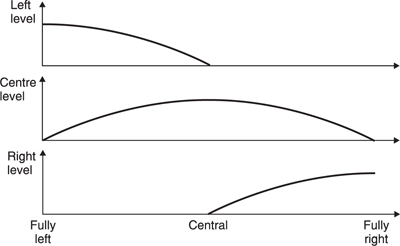
The use of the Centre speaker comes from cinema practice and is intended to deliver central images more accurately for listeners positioned off-axis or to compensate for loudspeakers with poor imaging ability. With precision loudspeakers having good imaging, there is little difference between the performance of a Left, Centre, Right system and a simple Left, Right stereo system where the centre channel has been equally added to the Left and Right signals.
A front virtual image can be located anywhere between the Left and Right speakers, and by a similar argument a rear virtual image can be located anywhere between the Left rear and Right rear speakers. It will be clear that this is possible simply by considering the head to be turned through 180° in Figure 5.73.
Five-channel surround sound is something of a misnomer because there is no mechanism by which a virtual sound source can be made to appear to the side. Figure 5.78 shows that images can be positioned between the front speakers or between the rear speakers only. If an attempt is made to position a sound source to the side by feeding equal amounts of signal into, say, the Left and Left rear speakers, the result will be unsatisfactory to a listener facing forward. The sound source will appear at the front or the rear depending on the position of the listener and may jump between these locations. Some writers have reported that sound appears to come from above and to the side.
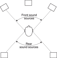
With surround, stereo and mono equipment co-existing, it is necessary to consider compatibility so that, for example, acceptable results are obtained when listening to surround material on stereo equipment, or stereo material on mono equipment.
Well-recorded surround sound material can be converted to stereo quite easily. The redundancy of the centre channel in surround means that it the centre signal is added equally to the left and right signals, a good central image will still be obtained with good loudspeakers. Adding the rear channels to the appropriate front channels means that ambience and reverberation is still reproduced. It is possible for certain effects which rely on phase or time delay to succeed in surround but to produce artifacts in stereo. It is worth while monitoring in stereo at some point in a surround production to avoid such pitfalls.
There is a certain amount of compatibility between intensity stereo and mono systems. If the S gain of a stereo signal is set to zero, only the M signal will pass. This is the component of the stereo image due to sounds from straight ahead and is the signal used when monophonic audio has to be produced from stereo.
Sources positioned on the extreme edges of the sound stage will not appear as loud in mono as those in the centre and any antiphase ambience will cancel out, but in most cases the result is adequate. Clearly an accidental situation in which one channel is phase reversed is catastrophic in mono as the centre of the image will be cancelled out. Stereo signals from spaced microphones generally have poor mono compatibility because of comb filtering.
One characteristic of stereo is that the viewer is able to concentrate on a sound coming from a particular direction using the cocktail party effect.
Thus it will be possible to understand dialog which is quite low in level even in the presence of other sounds in a stereo mix. In mono the listener will not be able to use spatial discrimination and the result may be reduced intelligibility which is particularly difficult for those with hearing impairments.13 Consequently it is good practice to monitor stereo material in mono to check for acceptable dialog.
A mono signal can also be reproduced on a stereo system by creating identical L and R signals, producing a central image only. Whilst there can be no real spatial information most people prefer mono on two speakers to mono on a single speaker.
5.15 Stereo and surround microphones
Pan-potted audio can never be as realistic as the results of using a stereo or surround microphone because the pan-pot causes all the sound to appear at one place in the stereo image. In the real world the direct sound should come from that location but reflections and reverberation should come from elsewhere. Artificial reverberation has to be used on panpotted mixes.
The job of a stereo microphone is to produce two audio signals which have no phase or time differences but whose relative levels are a function of the direction from which sound arrives. The most spatially accurate technique involves the use of directional microphones which are coincidentally mounted but with their polar diagrams pointing in different directions. This configuration is known variously as a crossed pair, a coincident pair or a Blumlein pair after Alan Blumlein14 who pioneered stereophony. Figure 5.79 shows a stereo microphone constructed by crossing a pair of figure-of-eight microphones at 90°.
The output from the two microphones will be equal for a sound source straight ahead, but as the source moves left, the output from the leftfacing microphone will increase and the output from the right-facing microphone will reduce. When a sound source has moved 45° off-axis, it will be in the response null of one of the microphones and so only one loudspeaker will emit sound. Thus the fully left or fully right reproduction condition is reached at ±45°. The angle between nulls in L and R is called the acceptance angle which has some parallels with the field of view of a camera.
Sounds between 45° and 135° will be emitted out of phase and will not form an identifiable image. Important sound sources should not be placed in this region. Sounds between 135° and 225° are in-phase and are mapped onto the frontal stereo image. The all-round pickup of the crossed eight makes it particularly useful for classical music recording where it will capture the ambience of the hall.
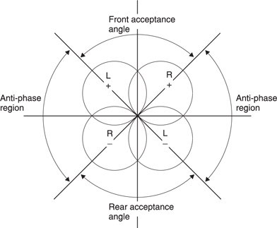
Other polar diagrams can be used, for example the crossed cardioid, shown in Figure 5.80 is popular. There is no obvious correct angle at which cardioids should be crossed, and the actual angle will depend on the application. Commercially available stereo microphones are generally built on the side-fire principle with one capsule vertically above the other.
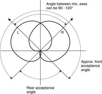
Figure 5.80 Crossed cardioid microphone.
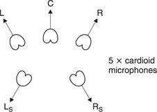
The two capsules can be independently rotated to any desired angle. Usually the polar diagrams of the two capsules can be changed.
For surround sound, an array of microphones will be needed. Figure 5.81 shows that one approach is to use five cardioid microphones. The rear microphones can be conventional cardioids, but it is advantageous if the front microphones are given a hyper-cardioid bias to narrow their directivity pattern. The microphones should not be turned outwards too far otherwise sounds to the side may result in problematic equal outputs in the front and rear channels.
In the soundfield microphone, four capsules are fitted in a tetrahedron. By adding and subtracting proportions of these four signals in various ways it is possible to synthesize a stereo microphone having any acceptance angle and to point it in any direction relative to the body of the microphone. This can be done using the control box supplied with the microphone. Although complex, the soundfield microphone has the advantage that it can be electrically steered and so no physical access is needed after it is slung. If all four outputs are recorded, the steering process can be performed in post-production by connecting the control box to the recorder output. For surround sound purposes, additional matrices allow the same four signals to be used to synthesize further stereo microphones. If the directivities are carefully determined, Left, Centre and Right signals can be derived as well as the rear pair.
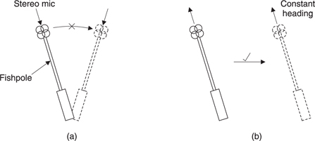
Figure 5.82 (a) Swinging a fishpole causes sound image to rotate. Tracking has to be used as in (b).
Clearly the use of stereo or surround sound will make it obvious if a microphone has been turned. In many applications the microphone is turned as a side effect of swinging a boom or fishpole, as in Figure 5.82(a). This is undesirable, and more precise handling techniques are necessary to keep the microphone heading constant as in (b).
5.16 M–S stereo
In audio production the apparent width of the stereo image may need to be adjusted, especially in television to obtain a good audio transition where there has been a change of shot or to match the sound stage to the picture. This can be done using M–S stereo and manipulating the difference between the two channels. Figure 5.83(a) shows that the two signals from the microphone, L and R, are passed through a sum and difference unit which produces two signals, M and S. The M or Mid signal is the sum of L and R whereas the S or Side signal is the difference between L and R. The sums and differences are divided by two to keep the levels correct. These processes can be performed in the analog domain prior to conversion, or in the digital domain using the techniques shown in Chapter 2.
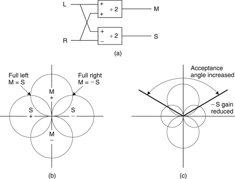
Figure 5.83 (a) M–S working adds and subtracts the L, R stereo signals to produce Mid and Side signals. In the case of a crossed eight, the M–S format is the equivalent of forward and sideways facing eights. (c) Changing the S gain alters the acceptance angle of the stereo microphone.
The result of this sum-difference process can be followed in Figure 5.83(b). A new polar diagram is drawn which represents the sum of L and R for all angles of approach. It will be seen that this results in a forwardfacing eight, as if a monophonic microphone had been used, hence the term M or Mid. If the same process is performed using L–R, the result is a sideways-facing eight, hence the term S or Side. In L, R format the acceptance angle is between the nulls whereas in M–S format the acceptance angle is between the points where the M and S polar diagrams cross.
The S signal can now be subject to variable gain. Following this a second sum and difference unit is used to return to L, R format for monitoring. The S gain control effectively changes the size of the S polar diagram without affecting the M polar diagram. Figure 5.83(c) shows that reducing the S gain makes the acceptance angle wider whereas increasing the S gain makes it smaller. Clearly if the S gain control is set to unity, there will be no change to the signals.
Whilst M–S stereo can be obtained by using a conventional L, R microphone and a sum and difference network, it is clear from Figure 5.83(b) that M–S signals can be obtained directly using a suitable microphone. Figure 5.84 shows a number of M–S microphones in which the S capsule is always an eight. A variety of responses (other than omni) can be used for the M capsule.
The M–S microphone technique has a number of advantages. The narrowing polar diagram at high frequencies due to diffraction is less of a problem because the most prominent sound source will generally be in the centre of the stereo image and this is directly on the axis of the M capsule. An image width control can easily be built into an M–S microphone. A favourite mono microphone can be turned into an M–S microphone simply by mounting a side-facing eight above it.
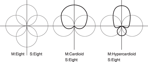
Figure 5.84 Various M–S microphone configurations. Note that the S microphone must always be an eight.
In surround sound, M–S techniques can be used directly for width control working on the rear speakers. In the case of the Left, Centre, Right speakers, increasing the level of the centre speaker whilst reducing those of the outer speakers will have the effect of reducing width.
5.17 Digitizing audio
As was introduced in Chapter 4, digitizing audio requires a number of processing stages. The analog signal from, for example, a microphone is subject to bandwidth limiting in an anti-aliasing filter, followed by sampling and quantizing to produce two’s complement coded PCM data. The quality obtained will be affected by the all three of these stages and the necessary quality will be considered here.
Sampling theory is only the beginning of the process which must be followed to arrive at a suitable sampling rate. As was seen in section 4.3, the finite slope of realizable filters will compel designers to raise the sampling rate above the theoretical value. For consumer products, the lower the sampling rate, the better, since the cost of the medium is directly proportional to the sampling rate: thus sampling rates near to twice 20 kHz are to be expected.
Early digital audio recorders were built before modern high-density digital media were available. These were based on analog video recorders which were adapted to store audio samples by creating a signal called pseudo-video which could convey binary as black and white levels. The sampling rate of such a system is constrained to relate simply to the field rate and field structure of the television standard used, so that an integer number of samples can be stored on each usable TV line in the field. Such a recording can be made on a monochrome recorder, and these recordings are made in two standards, 525 lines at 60 Hz and 625 lines at 50 Hz. Thus it is possible to find a frequency which is a common multiple of the two and also suitable for use as a sampling rate.
The allowable sampling rates in a pseudo-video system can be deduced by multiplying the field rate by the number of active lines in a field (blanked lines cannot be used) and again by the number of samples in a line. By careful choice of parameters it is possible to use either 525/60 or 625/50 video with a sampling rate of 44.1 kHz.
In 60 Hz video, there are 35 blanked lines, leaving 490 lines per frame, or 245 lines per field for samples. If three samples are stored per line, the sampling rate becomes
60 × 245 × 3 = 44.1 kHz
In 50 Hz video, there are 37 lines of blanking, leaving 588 active lines per frame, or 294 per field, so the same sampling rate is given by
50.00 × 294 × 3 = 44.1 kHz
The sampling rate of 44.1 kHz came to be that of the Compact Disc. Even though CD has no video circuitry and today the production and mastering equipment is based on data technology, the standard sampling rate remains.
For landlines to FM stereo broadcast transmitters having a 15 kHz audio bandwidth, the sampling rate of 32 kHz is more than adequate, and has been in use for some time in the United Kingdom and Japan. This frequency is also in use in DVB audio and in DAB.
The professional sampling rate of 48 kHz was proposed as having a simple relationship to 32 kHz, being far enough above 40 kHz to allow for high-quality filters or variable-speed operation. Recently there have been proposals calling for dramatically increased audio sampling rates. These are misguided and will not be considered further here.
The signal-to-noise ratio obtained by a convertor cannot exceed a figure which is set by the output PCM wordlength. Chapter 4 showed how this is calculated as a function of the dither technique employed, although a useful rule of thumb is simply to multiply the wordlength by six to get an SNR in dB. For consumer purposes, sixteen bits is generally adequate for post-produced material. For professional purposes longer wordlengths are used to give some freedom in level setting and to allow sixteen-bit performance after generation loss in production steps.
5.18 Audio convertors
The DAC will be discussed first, since ADCs often use embedded DACs in feedback loops. The purpose of a digital-to-analog convertor is to take numerical values and reproduce the continuous waveform that they represent. The conversion techniques shown in Chapter 4 are simply not accurate enough for audio use where wordlengths of sixteen bits or more are required. Although PCM audio is universal because of the ease with which it can be recorded and processed numerically, there are several alternative related methods of converting an analog waveform to a bitstream. The output of these convertor types is not Nyquist rate PCM, but this can be obtained from them by appropriate digital signal processing. In advanced conversion systems it is possible to adopt an alternative convertor technique specifically to take advantage of a particular characteristic. The output is then digitally converted to Nyquist rate PCM in order to obtain the advantages of both.
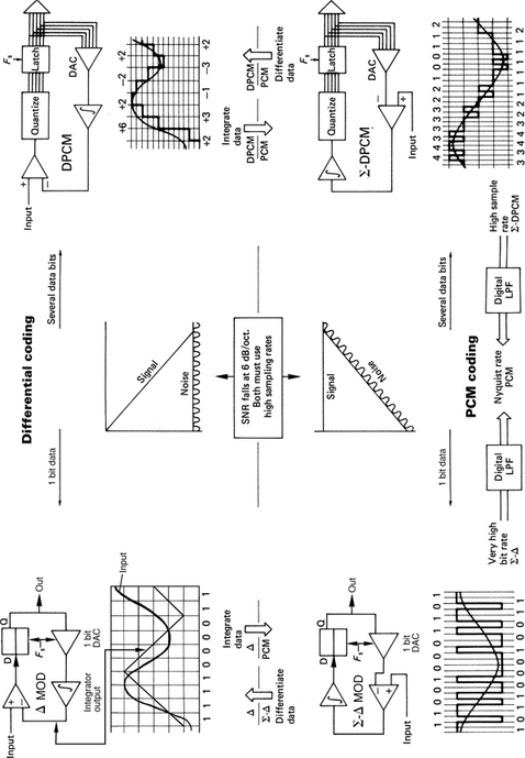
Figure 5.85 The four main alternatives to simple PCM conversion are compared here. Delta modulation is a one-bit case of differential PCM and conveys the slope of the signal. The digital output of both can be integrated to give PCM. Δ–Σ (sigma–delta) is a one-bit case of Δ-DPCM. The application of integrator before differentiator makes the output pure PCM, but tilts the noise floor; hence these can be referred to as ‘noise-shaping’ convertors.
Figure 5.85 introduces the alternative convertor structures. The top half of the diagram shows convertors which are differential. In differential coding the value of the output code represents the difference between the current sample voltage and that of the previous sample. The lower half of the diagram shows convertors which are PCM. In addition, the left side of the diagram shows single-bit convertors, whereas the right side shows multi-bit convertors.
In differential pulse code modulation (DPCM), shown at top right, the difference between the previous absolute sample value and the current one is quantized into a multi-bit binary code. It is possible to produce a DPCM signal from a PCM signal simply by subtracting successive samples; this is digital differentiation. Similarly, the reverse process is possible by using an accumulator or digital integrator (see Chapter 2) to compute sample values from the differences received. The problem with this approach is that it is very easy to lose the baseline of the signal if it commences at some arbitrary time. A digital high-pass filter can be used to prevent unwanted offsets.
Differential convertors do not have an absolute amplitude limit. Instead there is a limit to the maximum rate at which the input signal voltage can change. They are said to be slew rate limited, and thus the permissible signal amplitude falls at 6 dB per octave. As the quantizing steps are still uniform, the quantizing error amplitude has the same limits as PCM. As input frequency rises, ultimately the signal amplitude available will fall down to it.
If DPCM is taken to the extreme case where only a binary output signal is available then the process is described as delta modulation (top left in Figure 5.85). The meaning of the binary output signal is that the current analog input is above or below the accumulation of all previous bits. The characteristics of the system show the same trends as DPCM, except that there is severe limiting of the rate of change of the input signal. A DPCM decoder must accumulate all the difference bits to provide a PCM output for conversion to analog, but with a one-bit signal the function of the accumulator can be performed by an analog integrator.
If an integrator is placed in the input to a delta modulator, the integrator’s amplitude response loss of 6 dB per octave parallels the convertor’s amplitude limit of 6 dB per octave; thus the system amplitude limit becomes independent of frequency. This integration is responsible for the term sigma–delta modulation, since in mathematics sigma is used to denote summation. The input integrator can be combined with the integrator already present in a delta-modulator by a slight rearrangement of the components (bottom left in Figure 5.85). The transmitted signal is now the amplitude of the input, not the slope; thus the receiving integrator can be dispensed with, and all that is necessary to alter the DAC is an LPF to smooth the bits. The removal of the integration stage at the decoder now means that the quantizing error amplitude rises at 6 dB per octave, ultimately meeting the level of the wanted signal.
The principle of using an input integrator can also be applied to a true DPCM system and the result should perhaps be called sigma DPCM (bottom right in Figure 5.85). The dynamic range improvement over delta–sigma modulation is 6 dB for every extra bit in the code. Because the level of the quantizing error signal rises at 6 dB per octave in both delta–sigma modulation and sigma DPCM, these systems are sometimes referred to as ‘noise-shaping’ convertors, although the word ‘noise’ must be used with some caution. The output of a sigma DPCM system is again PCM, and a DAC will be needed to receive it, because it is a binary code.
As the differential group of systems suffer from a wanted signal that converges with the unwanted signal as frequency rises, they must all use very high sampling rates.15 It is possible to convert from sigma DPCM to conventional PCM by reducing the sampling rate digitally. When the sampling rate is reduced in this way, the reduction of bandwidth excludes a disproportionate amount of noise because the noise shaping concentrated it at frequencies beyond the audio band. The use of noise shaping and oversampling is the key to the high resolution obtained in advanced convertors.
5.19 Oversampling in audio
Oversampling means using a sampling rate which is greater (generally substantially greater) than the Nyquist rate. Neither sampling theory nor quantizing theory require oversampling to be used to obtain a given signal quality, but Nyquist rate conversion places extremely high demands on component accuracy and analog filter performance when a convertor is implemented. Oversampling allows a given signal quality to be reached without requiring very close tolerance, and therefore expensive, components. Although it can be used alone, the advantages of oversampling are better realized when it is used in conjunction with noise shaping. Thus in practice the two processes are generally used together and the terms are often seen used in the loose sense as if they were synonymous. For a detailed and quantitative analysis of oversampling having exhaustive references the serious reader is referred to Hauser.16
In section 3.16, where dynamic element matching was described, it was seen that component accuracy was traded for accuracy in the time domain. Oversampling is another example of the same principle.
Figure 5.86 shows the main advantages of oversampling. At (a) it will be seen that the use of a sampling rate considerably above the Nyquist rate allows the anti-aliasing and reconstruction filters to be realized with a much more gentle cut-off slope. There is then less likelihood of phase linearity and ripple problems in the audio passband.
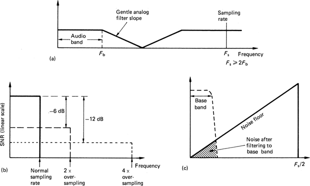
Figure 5.86(b) shows that information in an analog signal is twodimensional and can be depicted as an area which is the product of bandwidth and the linearly expressed signal-to-noise ratio. The figure also shows that the same amount of information can be conveyed down a channel with a SNR of half as much (6 dB less) if the bandwidth used is doubled, with 12 dB less SNR if bandwidth is quadrupled, and so on, provided that the modulation scheme used is perfect.
The information in an analog signal can be conveyed using some analog modulation scheme in any combination of bandwidth and SNR which yields the appropriate channel capacity. If bandwidth is replaced by sampling rate and SNR is replaced by a function of wordlength, the same must be true for a digital signal as it is no more than a numerical analog. Thus raising the sampling rate potentially allows the wordlength of each sample to be reduced without information loss.
Oversampling permits the use of a convertor element of shorter wordlength, making it possible to use a flash convertor. The flash convertor is capable of working at very high frequency and so large oversampling factors are easily realized. The flash convertor needs no track/hold system as it works instantaneously. If the sigma-DPCM convertor structure of Figure 5.85 is realized with a flash convertor element, it can be used with a high oversampling factor. Figure 5.86(c) shows that this class of convertor has a rising noise floor. If the highly oversampled output is fed to a digital low-pass filter which has the same frequency response as an analog anti-aliasing filter used for Nyquist rate sampling, the result is a disproportionate reduction in noise because the majority of the noise was outside the audio band. A high-resolution convertor can be obtained using this technology without requiring unattainable component tolerances.
Information theory predicts that if an audio signal is spread over a much wider bandwidth by, for example, the use of an FM broadcast transmitter, the SNR of the demodulated signal can be higher than that of the channel it passes through, and this is also the case in digital systems. The concept is illustrated in Figure 5.87. At (a) four-bit samples are delivered at sampling rate F. As four bits have sixteen combinations, the information rate is 16 F. At (b) the same information rate is obtained with three-bit samples by raising the sampling rate to 2 F and at (c) two-bit samples having four combinations require to be delivered at a rate of 4 F. Whilst the information rate has been maintained, it will be noticed that the bit-rate of (c) is twice that of (a). The reason for this is shown in Figure 5.88. A single binary digit can only have two states; thus it can only convey two pieces of information, perhaps ‘yes’ or ‘no’. Two binary digits together can have four states, and can thus convey four pieces of information, perhaps ‘spring summer autumn or winter’, which is two pieces of information per bit. Three binary digits grouped together can have eight combinations, and convey eight pieces of information, perhaps ‘doh re mi fah so lah te or doh’, which is nearly three pieces of information per digit. Clearly the further this principle is taken, the greater the benefit. In a sixteen-bit system, each bit is worth 4 K pieces of information. It is always more efficient, in information-capacity terms, to use the combinations of long binary words than to send single bits for every piece of information. The greatest efficiency is reached when the longest words are sent at the slowest rate which must be the Nyquist rate. This is one reason why PCM recording is more common than delta modulation, despite the simplicity of implementation of the latter type of convertor. PCM simply makes more efficient use of the capacity of the binary channel.
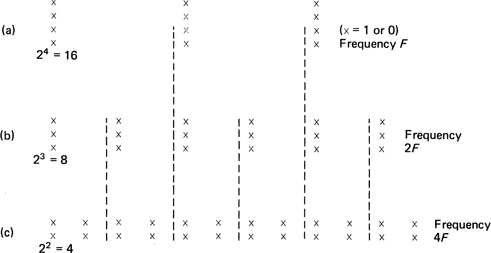
Figure 5.87 Information rate can be held constant when frequency doubles by removing one bit from each word. In all cases here it is 16 F. Note bit rate of (c) is double that of (a). Data storage in oversampled form is inefficient.
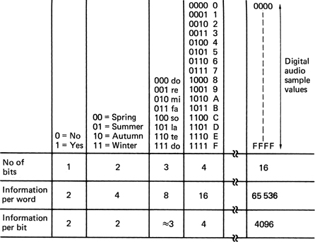
Figure 5.88 The amount of information per bit increases disproportionately as wordlength increases. It is always more efficient to use the longest words possible at the lowest word rate. It will be evident that sixteen bit PCM is 2048 times as efficient as delta modulation. Oversampled data are also inefficient for storage.
Oversampling is a method of overcoming practical implementation problems by replacing a single critical element or bottleneck by a number of elements whose overall performance is what counts. As Hauser16 properly observed, oversampling tends to overlap the operations which are quite distinct in a conventional convertor. In earlier sections of this chapter, the vital subjects of filtering, sampling, quantizing and dither have been treated almost independently. Figure 5.89(a) shows that it is possible to construct an ADC of predictable performance by a taking a suitable anti-aliasing filter, a sampler, a dither source and a quantizer and assembling them like building bricks. The bricks are effectively in series and so the performance of each stage can only limit the overall performance. In contrast Figure 5.89(b) shows that with oversampling the overlap of operations allows different processes to augment one another allowing a synergy which is absent in the conventional approach.
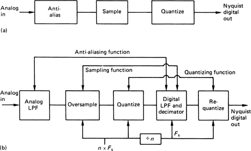
If the oversampling factor is n, the analog input must be bandwidth limited to n.Fs/2 by the analog anti-aliasing filter. This unit need only have flat frequency response and phase linearity within the audio band. Analog dither of an amplitude compatible with the quantizing interval size is added prior to sampling at n.Fs and quantizing.
Next, the anti-aliasing function is completed in the digital domain by a low-pass filter which cuts off at Fs/2. Using an appropriate architecture this filter can be absolutely phase-linear and implemented to arbitrary accuracy. Such filters are discussed in Chapter 4. The filter can be considered to be the demodulator of Figure 5.86 where the SNR improves as the bandwidth is reduced. The wordlength can be expected to increase. As Chapter 2 illustrated, the multiplications taking place within the filter extend the wordlength considerably more than the bandwidth reduction alone would indicate. The analog filter serves only to prevent aliasing into the audio band at the oversampling rate; the audio spectrum is determined with greater precision by the digital filter.
With the audio information spectrum now Nyquist limited, the sampling process is completed when the rate is reduced in the decimator. One sample in n is retained.
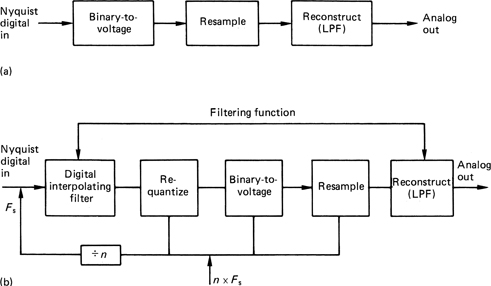
The excess wordlength extension due to the anti-aliasing filter arithmetic must then be removed. Digital dither is added, completing the dither process, and the quantizing process is completed by requantizing the dithered samples to the appropriate wordlength which will be greater than the wordlength of the first quantizer. Alternatively noise shaping may be employed.
Figure 5.90(a) shows the building-brick approach of a conventional DAC. The Nyquist rate samples are converted to analog voltages and then a steep-cut analog low-pass filter is needed to reject the sidebands of the sampled spectrum.
Figure 5.90(b) shows the oversampling approach. The sampling rate is raised in an interpolator which contains a low-pass filter that restricts the baseband spectrum to the audio bandwidth shown. A large frequency gap now exists between the baseband and the lower sideband. The multiplications in the interpolator extend the wordlength considerably and this must be reduced within the capacity of the DAC element by the addition of digital dither prior to requantizing. Again noise shaping may be used as an alternative.
If an oversampling convertor is considered which makes no attempt to shape the noise spectrum, it will be clear that if it contains a perfect quantizer, no amount of oversampling will increase the resolution of the system, since a perfect quantizer is blind to all changes of input within one quantizing interval, and looking more often is of no help. It was shown earlier that the use of dither would linearize a quantizer, so that input changes much smaller than the quantizing interval would be reflected in the output and this remains true for this class of convertor.
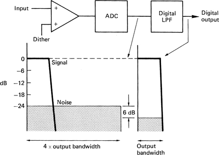
Figure 5.91 shows an example of a white-noise-dithered quantizer, oversampled by a factor of four. Since dither is correctly employed, it is valid to speak of the unwanted signal as noise. The noise power extends over the whole baseband up to the Nyquist limit. If the basebandwidth is reduced by the oversampling factor of four back to the bandwidth of the original analog input, the noise bandwidth will also be reduced by a factor of four, and the noise power will be onequarter of that produced at the quantizer. One-quarter noise power implies one-half the noise voltage, so the SNR of this example has been increased by 6 dB, the equivalent of one extra bit in the quantizer. Information theory predicts that an oversampling factor of four would allow an extension by two bits. This method is sub-optimal in that very large oversampling factors would be needed to obtain useful resolution extension, but it would still realize some advantages, particularly the elimination of the steep-cut analog filter.
The division of the noise by a larger factor is the only route left open, since all the other parameters are fixed by the signal bandwidth required. The reduction of noise power resulting from a reduction in bandwidth is only proportional if the noise is white, i.e. it has uniform power spectral density (PSD). If the noise from the quantizer is made spectrally non-uniform, the oversampling factor will no longer be the factor by which the noise power is reduced. The goal is to concentrate noise power at high frequencies, so that after low-pass filtering in the digital domain down to the audio input bandwidth, the noise power will be reduced by more than the oversampling factor.
5.20 Noise shaping
Noise shaping dates from the work of Cutler17 in the 1950s. It is a feedback technique applicable to quantizers and requantizers in which the quantizing process of the current sample is modified in some way by the quantizing error of the previous sample.
When used with requantizing, noise shaping is an entirely digital process which is used, for example, following word extension due to the arithmetic in digital mixers or filters in order to return to the required wordlength. It will be found in this form in oversampling DACs. When used with quantizing, part of the noise-shaping circuitry will be analog. As the feedback loop is placed around an ADC it must contain a DAC. When used in convertors, noise shaping is primarily an implementation technology. It allows processes which are conveniently available in integrated circuits to be put to use in audio conversion. Once integrated circuits can be employed, complexity ceases to be a drawback and low-cost mass-production is possible.
It has been stressed throughout this chapter that a series of numerical values or samples is just another analog of an audio waveform. Chapter 2 showed that all analog processes such as mixing, attenuation or integration all have exact numerical parallels. It has been demonstrated that digitally dithered requantizing is no more than a digital simulation of analog quantizing. It should be no surprise that in this section noise shaping will be treated in the same way. Noise shaping can be performed by manipulating analog voltages or numbers representing them or both. If the reader is content to make a conceptual switch between the two, many obstacles to understanding fall, not just in this topic, but in digital audio in general.
The term ‘noise shaping’ is idiomatic and in some respects unsatisfactory because not all devices which are called noise shapers produce true noise. The caution which was given when treating quantizing error as noise is also relevant in this context. Whilst ‘quantizing-errorspectrum shaping’ is a bit of a mouthful, it is useful to keep in mind that noise shaping means just that in order to avoid some pitfalls. Some noise-shaper architectures do not produce a signal-decorrelated quantizing error and need to be dithered.
Figure 5.92(a) shows a requantizer using a simple form of noise shaping. The low-order bits which are lost in requantizing are the quantizing error. If the value of these bits is added to the next sample before it is requantized, the quantizing error will be reduced. The process is somewhat like the use of negative feedback in an operational amplifier except that it is not instantaneous, but encounters a onesample delay. With a constant input, the mean or average quantizing error will be brought to zero over a number of samples, achieving one of the goals of additive dither. The more rapidly the input changes, the greater the effect of the delay and the less effective the error feedback will be. Figure 5.92(b) shows the equivalent circuit seen by the quantizing error, which is created at the requantizer and subtracted from itself one sample period later. As a result the quantizing error spectrum is not uniform, but has the shape of a raised sinewave shown at (c), hence the term ‘noise shaping’. The noise is very small at DC and rises with frequency, peaking at the Nyquist frequency at a level determined by the size of the quantizing step. If used with oversampling, the noise peak can be moved outside the audio band.
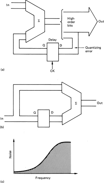
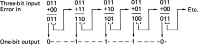
Figure 5.93 By adding the error caused by truncation to the next value, the resolution of the lost bits is maintained in the duty cycle of the output. Here, truncation of 011 by two bits would give continuous zeros, but the system repeats 0111, 0111, which, after filtering, will produce a level of three-quarters of a bit.
Figure 5.93 shows a simple example in which two low-order bits need to be removed from each sample. The accumulated error is controlled by using the bits which were neglected in the truncation, and adding them to the next sample. In this example, with a steady input, the roundoff mechanism will produce an output of 01110111 . . . If this is low-pass filtered, the three ones and one zero result in a level of three-quarters of a quantizing interval, which is precisely the level which would have been obtained by direct conversion of the full digital input. Thus the resolution is maintained even though two bits have been removed.
Noise shaping can also be used without oversampling. In this case the noise cannot be pushed outside the audio band. Instead the noise floor is shaped or weighted to complement the unequal spectral sensitivity of the ear to noise18,19. Unless we wish to violate Shannon’s theory, this psychoacoustically optimal noise shaping can only reduce the noise power at certain frequencies by increasing it at others. Thus the average log psd over the audio band remains the same, although it may be raised slightly by noise induced by imperfect processing.
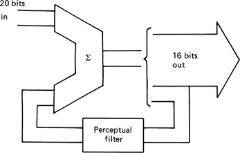
Figure 5.94 shows noise shaping applied to a digitally dithered requantizer. Such a device might be used when, for example, making a CD master from a twenty-bit recording format. The input to the dithered requantizer is subtracted from the output to give the error due to requantizing. This error is filtered (and inevitably delayed) before being subtracted from the system input. The filter is not designed to be the exact inverse of the perceptual weighting curve because this would cause extreme noise levels at the ends of the band. Instead the perceptual curve is levelled off20 such that it cannot fall more than e.g. 40 dB below the peak.
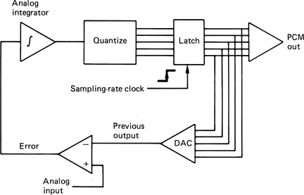
Figure 5.95 The sigma-DPCM convertor of Figure 5.85 is shown here in more detail.
Psychoacoustically optimal noise shaping can offer nearly three bits of increased dynamic range when compared with optimal spectrally flat dither. Enhanced Compact Discs recorded using these techniques are now available.
The sigma-DPCM convertor introduced above works well with noise shaping and is shown in more detail in Figure 5.95. The current digital sample from the quantizer is converted back to analog in the embedded DAC. The DAC output differs from the ADC input by the quantizing error. The DAC output is subtracted from the analog input to produce an error which is integrated to drive the quantizer in such a way that the error is reduced. With a constant input voltage the average error will be zero because the loop gain is infinite at DC. If the average error is zero, the mean or average of the DAC outputs must be equal to the analog input. The instantaneous output will deviate from the average in what is called an idling pattern. The presence of the integrator in the error feedback loop makes the loop gain fall with rising frequency. With the feedback falling at 6 dB per octave, the noise floor will rise at the same rate.
A greater improvement in dynamic range can be obtained if the integrator is supplanted to realize a higher-order filter.21 The filter is in the feedback loop and so the noise will have the opposite response to the filter and will therefore rise more steeply to allow a greater SNR enhancement after decimation. Figure 5.96 shows the theoretical SNR enhancement possible for various loop filter orders and oversampling factors. A further advantage of high-order loop filters is that the quantizing noise can be decorrelated from the signal making dither unnecessary. High-order loop filters were at one time thought to be impossible to stabilize, but this is no longer the case, although care is necessary. One technique which may be used is to include some feedforward paths as shown in Figure 5.97.
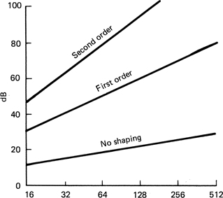
Figure 5.96 The enhancement of SNR possible with various filter orders and oversampling factors in noise-shaping convertors.
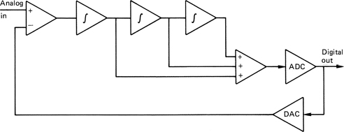
References
1. Martin, W.H., Decibel – the new name for the transmission unit. Bell System Tech. J. (Jan. 1929)
2. Moore, B.C.J., An Introduction to the Psychology of Hearing, London: Academic Press (1989)
3. Muraoka, T., Iwahara, M. and Yamada, Y., Examination of audio bandwidth requirements for optimum sound signal transmission. J. Audio Eng. Soc., 29, 2–9 (1982)
4. Muraoka, T., Yamada, Y. and Yamazaki, M., Sampling frequency considerations in digital audio. J. Audio Eng. Soc., 26, 252–256 (1978)
5. Fincham, L.R., The subjective importance of uniform group delay at low frequencies. Presented at the 74th Audio Engineering Society Convention, New York (1983), Preprint 2056 (H-1)
6. Fletcher, H., Auditory patterns. Rev. Modern Physics, 12, 47–65 (1940)
7. Carterette, E.C. and Friedman, M.P., Handbook of Perception, 305–319, New York: Academic Press (1978)
8. Moore, B.C., An Introduction to the Psychology of Hearing, section 6.12, London: Academic Press (1989)
9. Cao, Y., Sridharan, S. and Moody, M., Co-talker separation using the cocktail party effect. J. Audio Eng. Soc., 44, No.12, 1084–1096 (1996)
10. Moore, B.C., An Introduction to the Psychology of Hearing, section 6.13, London: Academic Press (1989)
11. AES Anthology: Microphones, New York: Audio Engineering Society
12. Bauer, B.B., A century of microphones. J. Audio Eng. Soc., 35, 246–258 (1967)
13. Harvey, F.K. and Uecke, E.H., Compatibility problems in two channel stereophonic recordings. J. Audio Eng. Soc., 10, No 1, 8–12 (Jan. 1962)
14. Alexander, R.C., The Life and Works of Alan Dower Blumlein, Oxford: Focal Press (1999)
15. Adams, R.W., Companded predictive delta modulation: a low-cost technique for digital recording. J. Audio Eng. Soc., 32, 659–672 (1984)
16. Hauser, M.W., Principles of oversampling A/D conversion. J. Audio Eng. Soc., 39, 3–26 (1991)
17. Cutler, C.C., Transmission systems employing quantization. US Pat. No. 2.927,962 (1960)
18. Fielder, L.D., Human auditory capabilities and their consequences in digital audio convertor design. In Audio in Digital Times, New York: AES (1989)
19. Wannamaker, R.A., Psychoacoustically optimal noise shaping. J. Audio Eng. Soc., 40, 611–620 (1992)
20. Lipshitz, S.P., Wannamaker, R.A. and Vanderkooy, J., Minimally audible noise shaping. J. Audio Eng. Soc., 39, 836–852 (1991)
21. Adams, R.W., Design and implementation of an audio 18-bit A/D convertor using oversampling techniques. Presented at the 77th Audio Engineering Society Convention, Hamburg (1985), Preprint 2182