6. format worksheets
Although the information in our four worksheets is accurate and informative, it doesn’t look very good. And in this day and age, looks are almost everything. We need to dress these worksheets up to make them more presentable.
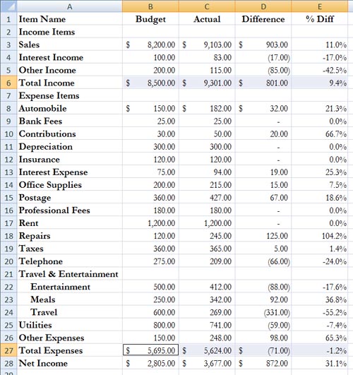
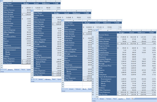
Excel offers many extremely flexible formatting options. Our worksheets can benefit from some font and number formatting, as well as alignment, borders, and color. As shown here, we’ll transform our plain Jane worksheets into worksheets that demand attention.
On the following pages, I’ll show you how to apply formatting to the January worksheet. You can repeat those steps on your own for the other worksheets in our workbook.
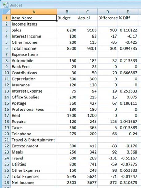
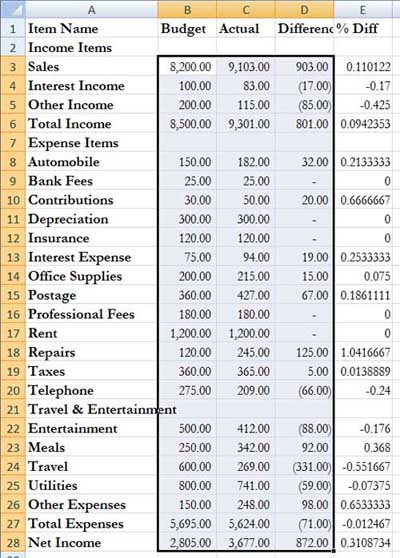
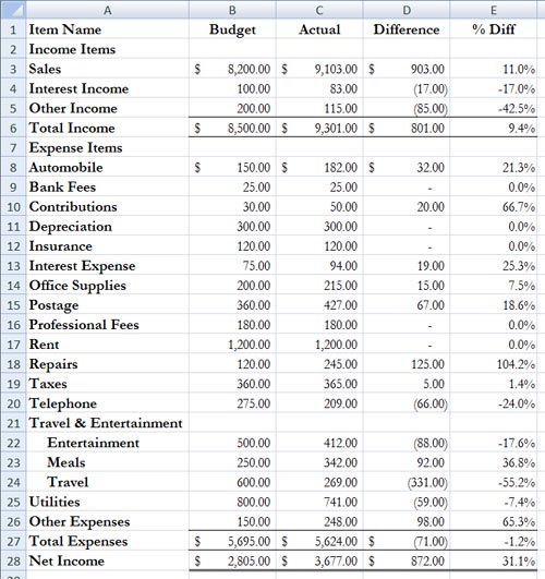
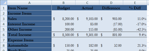
Before

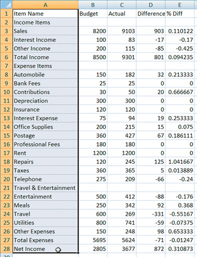
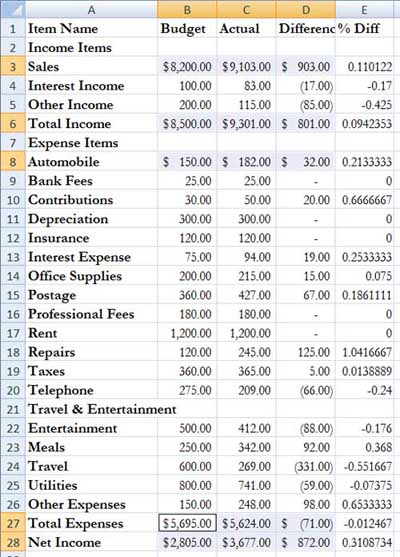
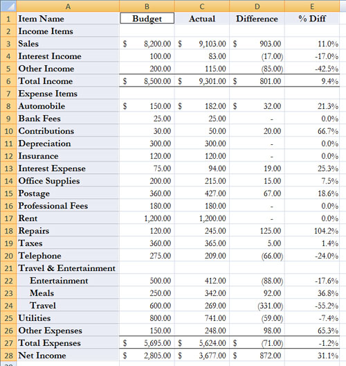
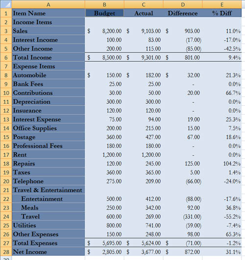
After
set font formatting
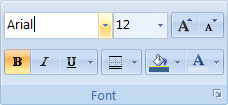
Font formatting changes the way individual characters of text appear. By default, Excel 2007 for Windows Vista uses 11 point Calibri font. You can change the font settings applied to any combination of worksheet cells.
In our worksheets, we’ll make the column and row headings bold and larger so they really stand out. We’ll also change the font applied to the entire worksheet to something a little more interesting.
1. Drag to select cells A1 to A28.
2. Hold down the Ctrl key and drag to add cells B1 to E1 to the selection.
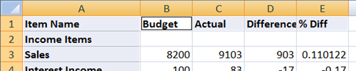
3. Click the Bold button in the Font group of the Ribbon’s Home tab.

The text in the selected cells turns bold.
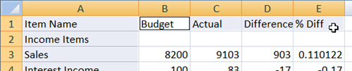
4. Choose 12 from the Font Size drop-down list in the Font group of the Ribbon’s Home tab.
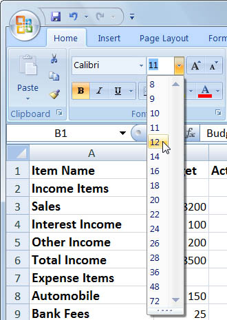
The text in the selected cells gets larger.
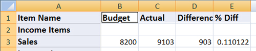
6. Choose Garamond from the Font drop-down list in the Font group of the Ribbon’s Home tab.
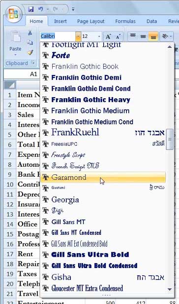
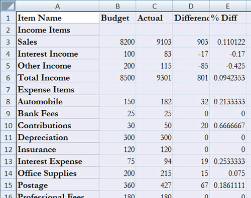
The text in the selected cells changes to the Garamond font.
format values
The dollar amounts in our worksheets would be a lot easier to read with commas and dollar signs.
1. Drag to select cells B3 to D28.
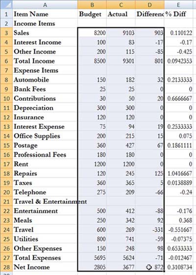
2. Click the Comma Style button in the Number group of the Ribbon’s Home tab.

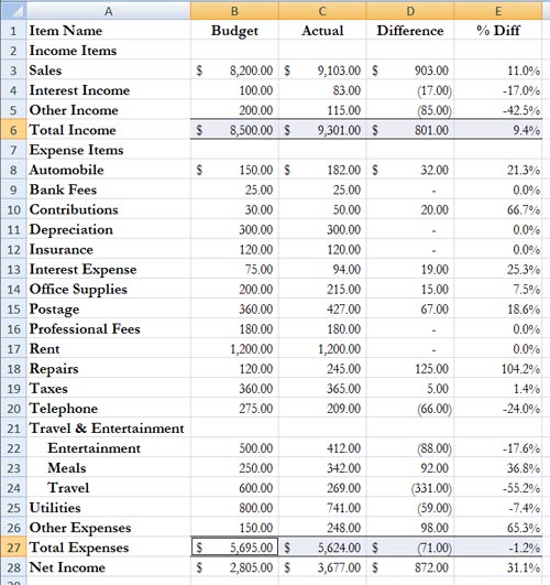
Commas, decimal places, and parentheses (for negative numbers) appear, as needed, for all values in selected cells.
3. Drag to select cells B3 to D3, B6 to D6, B8 to D8, and B27 to D28. Remember you must hold down the Ctrl key to select multiple ranges.
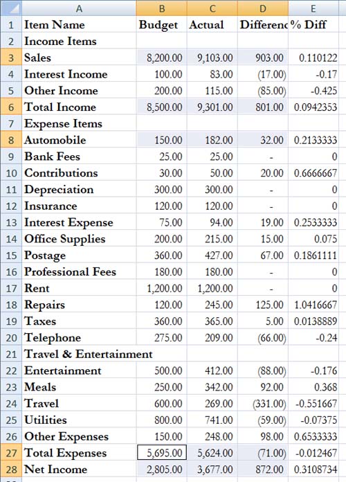
4. Click the Accounting Number Format button in the Number group of the Ribbon’s Home tab.
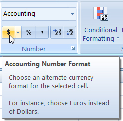
Currency symbols appear beside values in the selected cells.
format percentages
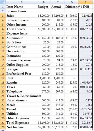
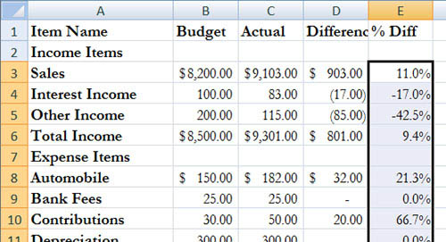
We can also use number formatting to format the percentages in column E so they look like percentages.
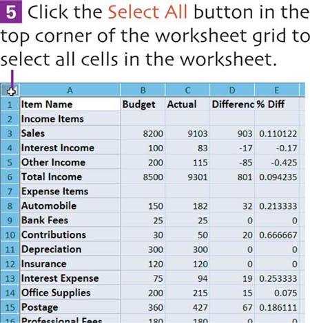
1. Drag to select all cells E3 to E28.
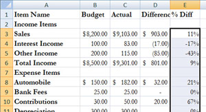
2. Click the Percent Style button in the Number group of the Ribbon’s Home tab.
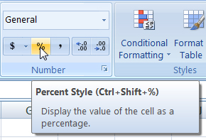
The numbers are formatted as percentages without any decimal places.
3. Click the Increase Decimal button in the Number group of the Ribbon’s Home tab.
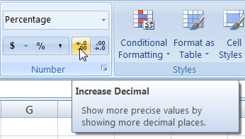
The numbers are reformatted so there’s one decimal place.
set column widths
When you create a worksheet, Excel automatically sets a default width for columns: 8.11 characters (or 80 pixels).
We’ve already used the AutoFit feature to increase the width of column A so its text fits in the column. And you may have noticed that Excel widened one or two columns to accommodate the number formatting we applied.
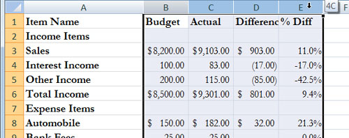
Now we’ll make column A a little wider again—remember, we increased the text size and applied bold formatting which made the text take up more space. We’ll also set the width of columns B, C, D, and E to a consistent wider setting.
1. Double-click the right border of column A.
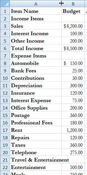
The column automatically widens again to accommodate the widest text in the column.
3. Press the mouse button and drag to the right to select columns B, C, D, and E.
4. Choose Column Width from the Format menu in the Cells group of the Ribbon’s Home tab.
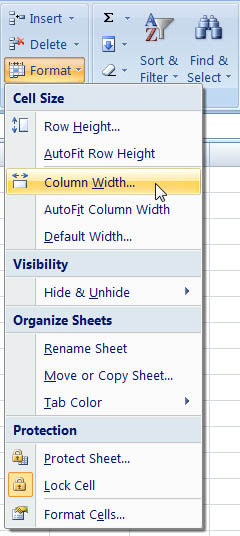
The Column Width dialog appears.
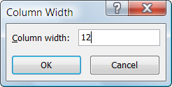
5. Enter 12 in the text box and click OK.
The columns widen.
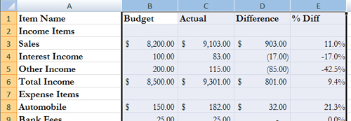
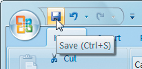
Save your work.
Now is a good time to click the Save button on the Quick Access toolbar to save your work up to this point.
set alignment
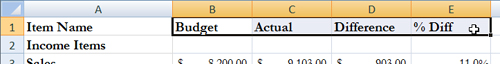
By default, text is left-aligned in a cell and a number (including a date or time) is right-aligned in a cell. For our worksheet, the headings at the top of columns B, C, D, and E might look better if they were centered.
1. Drag to select cells B1 through E1.
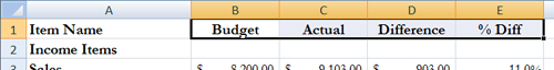
2. Click the Center button in the Alignment group of the Ribbon’s Home tab.
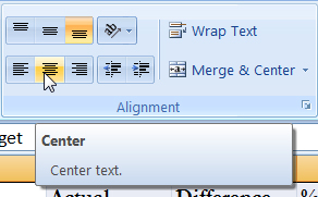
The cell contents are centered between the cell’s left and right boundaries.
indent text
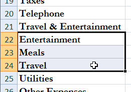
Entertainment, Meals, and Travel are three row headings that are part of the major Travel & Entertainment category of expenses. We can make that clear to the people who view the worksheet by indenting those three row headings.
1. Select cells A22 through A24.
2. Click the Increase Indent button in the Alignment group of the Ribbon’s Home tab twice.
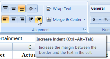
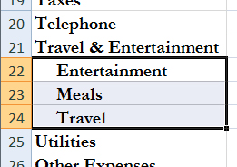
Each selected cell’s contents are shifted to the right.
add borders
Borders above and below the totals and net amounts would really help them stand out. We’ll add single lines above and below Income and Expense totals and a double line beneath the Net Income amounts.
1. Select cells B6 to E6, and B27 to E27. Remember, you must hold down the Control key to select multiple ranges.
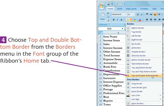
2. Choose Top and Bottom Border from the Borders menu in the Font group of the Ribbon’s Home tab.
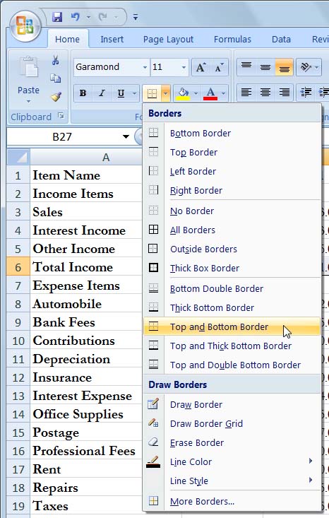
Borders are applied to the top and bottom of all selected cells.
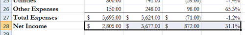
A double border appears beneath the selected cells.
Here’s what it should look like when you’re done, with the selection area removed:
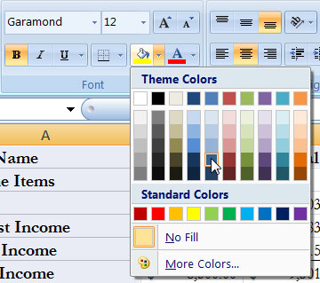
apply shading
Shading can also improve the appearance of a worksheet. We’ll apply dark colored shading to worksheet cells containing headings so they really stand out, then apply a lighter color shading to the rest of the worksheet.
1. Select cells A1 to E1 and A2 to A28. Remember, you must hold down the Control key to select multiple ranges.
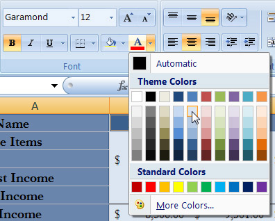
2. Choose a dark color from the Fill Color menu in the Font group of the Ribbon’s Home tab.
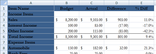
The color is applied to selected cells. Here’s what the top bunch of cells might look like with the selection area removed.
3. Select cells B2 to E28.

4. Choose a light color from the Fill Color menu in the Font group of the Ribbon’s Home tab.

The color is applied to selected cells.
change text color
When we applied dark shading to the worksheet’s headings, we created a problem: The black text may not be legible with the dark cell shading. We can fix this problem by making the heading text a lighter color.
1. Select cells A1 to E1 and A2 to A28. Remember, you must hold down the Control key to select multiple ranges.
2. Choose a light color from the Font Color menu in the Font group of the Ribbon’s Home tab.
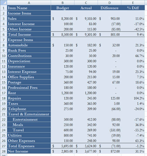
The color is applied to the font characters in selected cells. Here’s what the worksheet might look like with the selection area removed.
format all worksheets
So far, all we’ve done is format one of the four worksheets in our workbook file: January. You can follow the steps on pages 68-80 to apply the same formatting to the other worksheets in the file: February, March, and Quarter 1.
Here are a few things to keep in mind:
• To activate a worksheet, click its sheet tab.
• Not all worksheets have the same number of columns and rows, so you won’t be able to use the cell selections exactly as written in this chapter. Be sure to select the correct areas when applying formatting.
• In the February worksheet, Annual Party should be indented with the other Travel & Entertainment row headings.
• For the Quarter 1 worksheet, keep the consolidation’s detail hidden. You can also hide column B by setting its column width to 0 (zero).
extra bits
set font formatting pp. 68–69
• A font is basically a typeface.
• A point is a unit of measurement roughly equal to 1/72 of an inch. Fonts are measured in points. The bigger the point size, the bigger the characters.
• As you move the mouse pointer over items in the Font menu, the currently highlighted font is temporarily applied to selected cells. This makes it easy to preview what the cells will look like with that font applied.
• Another way to change the font or font size is to type a font name in the Font box (shown here) or value in the Font Size box and press Enter.
• Choose your font carefully! Some fonts are designed for display purposes only and can be difficult to read.
• Don’t get carried away with font formatting. Too much formatting can distract the reader.
• Want more font formatting options? Click the Dialog Box Launcher button in the lowerright corner of the Font group on the Ribbon’s Home tab.
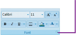
Then use the Font tab of the Format Cells dialog that appears to set font formatting options and click OK to apply them to selected cells.

format values pp. 70–71
• Another way to apply number formatting is with the Number Format menu in the Number group of the Ribbon’s Home tab.
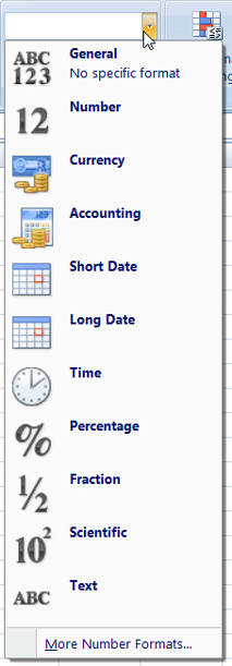
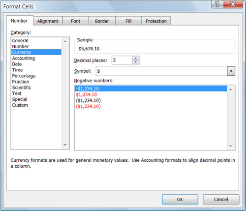
• For more number formatting options, click the Dialog Box Launcher button in the lowerright corner of the Number group in the Ribbon’s Home tab. Set options in the Number tab of the Format Cells dialog and click OK to apply formatting.
set column widths pp. 73–74
• Another way to change the width of a column is to drag the right edge of its column heading to the left or right.

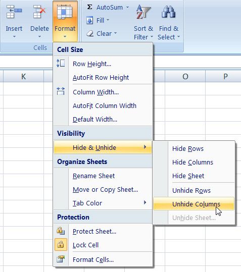
• You can hide a column by setting its width to 0 (zero) or by selecting it and choosing Hide Columns from the Hide & Unhide submenu on the Format menu in the Home tab’s Cells group. To unhide a column, select the columns on either side of it and choose Unhide Columns from the Hide & Unhide submenu on the Format menu in the Home tab’s Cells group.
set alignment p. 75
• Depending on column width settings, you may find that column headings look better when right-aligned over the numbers beneath them rather than centered. Click the Align Right button in the Alignment group of the Ribbon’s Home tab to try it and decide for yourself.
add borders p. 77–78
• Don’t confuse borders with underlines. Underlines are part of a cell’s font formatting and, when applied, appear only beneath characters in a cell. Borders appear for the entire width of the cell.
• Don’t confuse cell gridlines with borders, either. Gray cell gridlines appear onscreen to help you see cell boundaries. Normally, they don’t print—although you can elect to print them in the Page Setup dialog. Cell borders always print.
apply shading p. 79
• Although colored shading looks great onscreen and in color printouts, it doesn’t always look good in black and white printouts, which turn the colors to shades of gray. If you plan to print in black and white, you may want to minimize dark colored shading in your document.
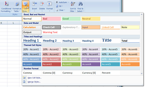
• Another way to apply shading is with Excel’s predefined styles. Choose one of the options in the Cell Styles menu in the Styles group of the Ribbon’s Home tab. The benefit of applying styles is that they automatically change text to a contrasting color if necessary.
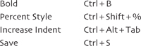
shortcut keys for this chapter