3. build the budget worksheet
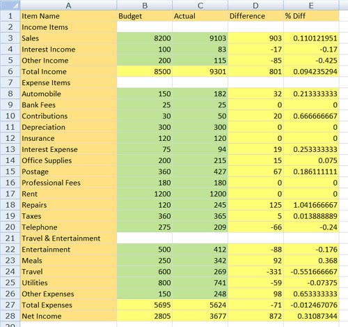
The primary element of our project is the monthly budget worksheet. This worksheet lists all of the income and expense categories with columns for budgeted amounts, actual amounts, dollar difference, and percent difference. It also includes subtotals and totals.
As you can see, an Excel worksheet window closely resembles an accountant’s paper worksheet. It includes columns and rows that intersect at cells. To build our budget worksheet, we’ll enter information into cells.
In this chapter, we’ll create the budget worksheet as shown here. (We’ll apply formatting to the worksheet so it looks more presentable later in this project.)

name the sheet
The sheet tabs at the bottom of the worksheet window enable you to identify the active sheet. Each new workbook file includes three worksheets named Sheet1, Sheet2, and Sheet3. You can change the name of a sheet to make it more descriptive.
It’s easy to identify the active sheet. Its sheet tab is white and the sheet name appears in bold text. And, if you have sharp eyes, you may notice that the active sheet’s tab seems to appear on top of the other tabs.
![]()
1. Double-click the Sheet1 sheet tab. The name of the tab becomes selected.
![]()
2. Type January. The text you type overwrites the selected sheet name.
![]()
3. Press Enter. The new name is saved.
![]()
understand references
The concept of references or addressing is important when working with spreadsheets. A reference or address identifies the part of the worksheet that you are working with.

Cells are referred to using the letter of the column and the number of the row.
enter information
To build the budget worksheet, you’ll enter three kinds of information into Excel worksheet cells:
• Labels (shown here in orange) are text entries that are used to identify information in the worksheet. For example, the word Budget is a label that will appear at the top of the column containing budget information.
• Values (shown here in green) are numbers, dates, or times. Values differ from labels in that you can perform mathematical calculations on them. In our budget worksheet, you’ll enter numbers as values for budget and actual information.
• Formulas (shown here in yellow) are calculations written in a special notation that Excel can understand. When you enter a formula in a cell, Excel displays the result of the formula, not the formula itself. Formulas are a powerful feature of spreadsheet programs because they can perform all kinds of simple and complex calculations for you. In our budget worksheet, we’ll use formulas to calculate the difference between budget and actual information in dollars and percents and to calculate column subtotals and totals.
activate a cell
To enter information into a cell, you must activate it. That means moving the cell pointer to the cell in which you want to enter a label, value, or formula.
There are lots of ways to move the cell pointer, but rather than bombard you with a lot of unnecessary options, I’ll tell you the two ways I use most.
Point and click:
1. Move the mouse pointer, which looks like a cross, over the cell you want to activate.

2. Press the mouse button once. The cell pointer moves to the cell you pointed to.

Use the arrow keys:
On the keyboard, press the arrow key corresponding to the direction you want the cell pointer to move.
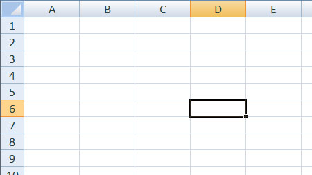
For example, in this illustration, if I wanted to move the cell pointer from cell C8 to cell D6...
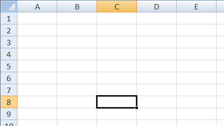
...I’d press the right arrow key once...

...and the up arrow key twice.
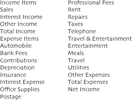
enter row headings
The row headings in our budget worksheet will identify the categories of income and expenses and label the subtotals and net income.
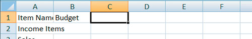
1. Activate cell A1 (the first cell in the worksheet).

2. Type Item Name.

3. Press Enter. The cell pointer moves down one cell.

4. Repeat steps 2 and 3 for the following labels:
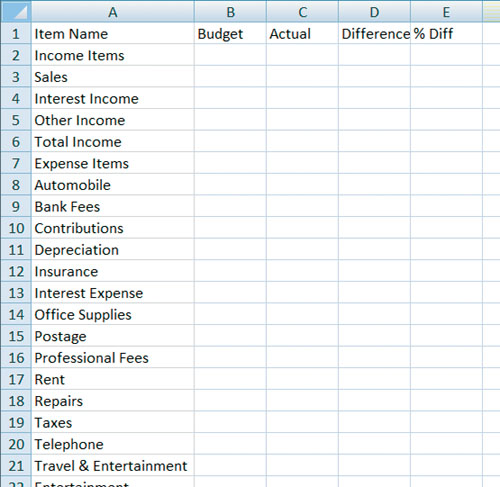
When you’re finished, the worksheet should look like this:

enter column headings
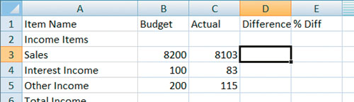
Our budget worksheet includes several columns of data and calculations. We’ll use column headings to identify them.
1. Activate cell B1 (the one to the right of where you entered Item Name).

2. Type Budget.

3. Press Tab. The cell pointer moves one cell to the right.
4. Repeat steps 2 and 3 for the following labels:
Actual
Difference
% Diff
When you’re finished, the worksheet should look like this:

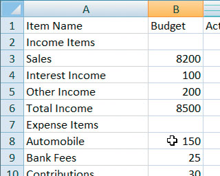
make a column wider

All the information you entered is still there; it’s just hidden because the column it’s in is too narrow. You can use Excel’s AutoWidth feature to quickly make a column wider.
1. Position the mouse pointer on the right border of column A. The mouse pointer turns into a bar with two arrows coming out of it.
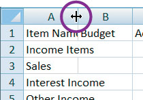
2. Double-click. The column automatically widens to accommodate the widest text in the column.
Have you been saving your work?
Now is a good time to click the Save button on the Quick Access toolbar to save your work up to this point.

enter values
The whole purpose of the worksheet is to compare budgeted to actual amounts. It’s time to enter those amounts. Since we need to enter values in two columns, we’ll use an entry selection area.
1. Position the mouse pointer over cell B3.

2. Press the mouse button down and drag down and to the right to cell C26. All cells between B3 and C26 are enclosed in a selection box, but cell B3 remains the active cell.

3. Type 8200.
It appears in cell B3.

4. Press Enter. Cell B4 becomes the active cell.

5. Repeat steps 3 and 4 for the remaining values in column B as shown here. When a cell that should remain blank becomes active, just press Enter again to make the next cell active. After entering the last value in the column, when you press Enter, cell C3 becomes active.

6. Repeat steps 3 and 4 for the values in column C as shown here. When a cell that should remain blank becomes active, just press Enter again to make the next cell active. After entering the last value in the column, when you press Enter, cell B3 becomes active again.
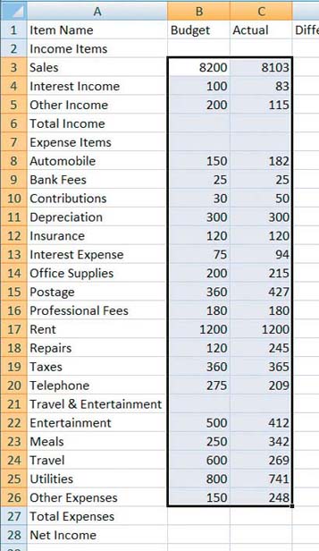
7. Click anywhere in the worksheet window to deselect the selected cells.
calculate a difference
Column D, which will display the difference between budgeted and actual amounts, will contain simple formulas that subtract one cell’s contents from another’s using cell references. In this step, we’ll write the first formula. Later, we’ll copy the formula to other cells in the column.
1. Activate cell D3.
2. Type =.

3. Click in cell C3.
Its cell reference appears in cell D3.

4. Type –.

5. Click in cell B3.
Its cell reference is appended to the formula in cell D3.

6. Press Enter.
The result of the formula you entered appears in cell D3.

calculate a percent diff
Column E calculates the percent difference between the budgeted and actual amounts. The percentage is based on the budgeted amount. We’ll write the first formula now and copy it to other cells in column E later.
1. Activate cell E3.

2. Type =.

3. Click in cell D3.
Its cell reference appears in cell E3.

4. Type /.

5. Click in cell B3.
Its cell reference is appended to the formula in cell E3.

6. Press Enter.
The result of the formula you entered appears in cell E3.

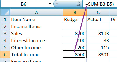
sum some values
Although you can write a formula that adds multiple cell references, one cell at a time, it’s much easier to use Excel’s SUM function to add up the contents of a range of cells. Here are two ways to enter the SUM function in formulas to create subtotals for the values in column B.
Use the AutoSum button:
1. Activate cell B6.

2. Click the AutoSum button in the Editing group of the Ribbon’s Home tab.

Excel writes a formula that uses the SUM function to add a range of cells. A colored box appears around the cells included in the formula.

3. If the formula is correct (as shown here), press Enter.

If the formula is not correct, type in the correct range reference and press Enter.
The result of the formula appears in cell B6.
Type and drag:

2. Type =SUM(.

3. Position the mouse pointer on cell B8.
4. Press the mouse button and drag down to cell B26. All cells you dragged over are selected and referenced in the formula in cell B27.
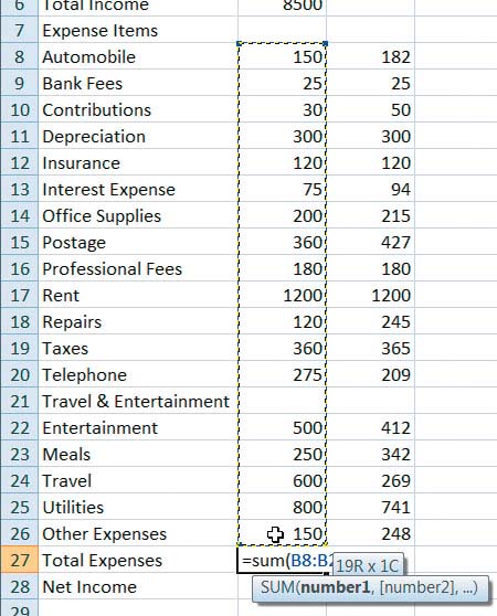
5. Type ).

6. Press Enter. The formula result appears in cell B27.
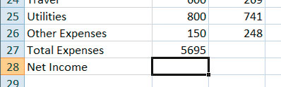
calculate net income
The final row of the worksheet contains cells to calculate the net income (total income minus total expenses). Here’s how to enter that final formula:
1. Activate cell B28.

2. Type =.

3. Click cell B6. Its reference appears in the formula in cell B28.

4. Type –.

5. Click cell B27. Its reference appears in the formula in cell B28.
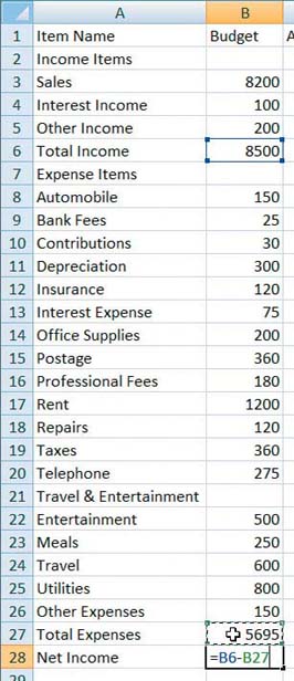
6. Press Enter. The result of the formula appears in cell B28.

Have you been saving your work?
Now is a good time to click the Save button on the Quick Access toolbar to save your work up to this point.
copy formulas
Excel lets you copy a formula in one cell to another cell that needs a similar formula. This can save a lot of time when building a worksheet with multiple columns or rows that need similar formulas.
For example, you can copy the formula in cell B6 (total income for budgeted amounts) to cell C6 (total income for actual amounts).

Similarly, you can copy the formula in cell D3 (difference between budgeted and actual sales) to D4 (difference between budgeted and actual interest income).

Excel automatically rewrites the cell references so they refer to the correct cells. You can view a cell’s formula by activating the cell and looking in the formula bar near the top of the window.

copy and paste
One way to copy formulas is with the Copy and Paste commands.
1. Drag to select cells D3 and E3.

2. Click the Copy button in the Clipboard group on the Ribbon’s Home tab.

A marquee appears around selected cells.

3. Activate cell D8.

4. Click the Paste button in the Clipboard group of the Ribbon’s Home tab.

The formulas in cells D3 and E3 are copied to cells D8 and E8. The marquee remains around the originally selected cells, indicating that they can be pasted elsewhere.

5. Activate cell D22.

6. Press Enter. The formulas are copied to cells D22 and E22. The marquee disappears, indicating the selection can no longer be pasted elsewhere.

use the fill handle
A quick way to copy the contents of one cell to one or more adjacent cells is with the fill handle. We’ll use the fill handle to finish up the worksheet entries.
1. Activate cell B6.

2. Position the mouse pointer on the selection’s fill handle—a tiny square in the bottom-right corner of the selection box. The mouse pointer turns into a black cross.

3. Press the mouse button and drag to the right. As you drag, a gray border stretches over the cells you pass over.

4. When the border surrounds cells B6 and C6, release the mouse button. The formula in cell B6 is copied to cell C6.
5. Repeat steps 1–4 for cell B27 to copy its formula to C27 and for cell B28 to copy its formula to cell C28. When you’re finished, the worksheet should look like this:
6. Drag to select cells D3 and E3.

7. Position the mouse pointer on the selection’s fill handle.
8. Press the mouse button down and drag so the border completely surrounds cells D3 through E6.

9. Release the mouse button. The two formulas are copied down to the cells you dragged over.

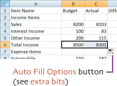
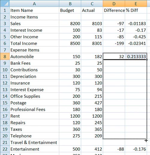
10. Repeat steps 6–9 to copy cells D8 and E8 to the range beneath it (shown here) and cells D22 and E22 to the range beneath it.
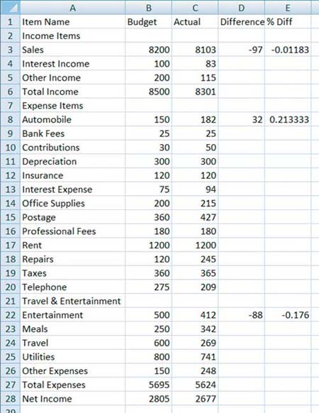
When you’re finished, the worksheet should look like this.
Have you been saving your work?
Now is a good time to click the Save button on the Quick Access toolbar to save your work up to this point.

change a value
In reviewing this worksheet, I realize that we made an error when entering values. The actual sales amount for the month wasn’t 8103 as we entered. It was really 9103! Better enter the correct value now.
1. Activate cell C3.

2. Type 9103. This new value overwrites the value already entered.

3. Press Enter.
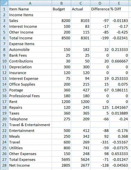
The value changes, but what’s more important is that all of the formulas that referenced that value, either directly or indirectly, also change. Compare the orange highlighted cells in this illustration with the same cells in the illustration on the previous page to see for yourself.
This is the reason we use spread- sheet programs!

extra bits
name the sheet p. 24
• As you’ll see in Chapter 8, you can instruct Excel to automatically display a sheet name in a printed report’s header or footer. That’s a good reason to give a sheet an appropriate name.
activate a cell p. 27
• When you use the point-andclick method for activating a cell, you must click. If you don’t click, the cell pointer won’t move and the cell you’re pointing to won’t be activated.
enter row headings p. 28
• When you enter text in a cell, Excel’s AutoComplete feature may suggest entries based on previous entries in the column.

To accept an entry, press Enter when it appears. Otherwise, just keep typing what you want to enter. The AutoComplete suggestion will eventually go away.
make a column wider p. 30
• You can’t change the width of a single cell. You must change the width of the entire column the cell is in.
enter values pp. 31–32
• You can enter any values you like in this step. But if you enter the same values I do, you can later compare the results of your formulas to mine to make sure the formulas you enter in the next step are correct.
• Do not include currency symbols or commas when entering values. Doing so will apply number formatting. I explain how to format cell contents, including values, in Chapter 6.
• If you use the arrow keys to move from one cell to the next, the selection area disappears. Although you can enter values without a selection area, using a selection area makes it easier to move from one cell to another.
• If, after entering values, you discover that one of the values is incorrect, activate the cell with the incorrect value, enter the correct value, and press Enter to save it.
calculate a difference p. 33
• In Excel, all formulas begin with an equal sign (=).
• Although you can write a formula that subtracts one number from another, using cell references in the formula ensures that the formula’s results remain correct, even if referenced cells’ values change.
• As our formula is written, if the actual amount is lower than the budgeted amount, the difference appears as a negative number. You can make this appear as a positive number by switching the order of the cell references so the formula is =B3-C3.
calculate a percent diff p. 34
• The number of decimal places that appear in the results of the formula depends on the width of the column the formula is in.
• Don’t worry that the percentages Excel calculates don’t look like percentages. Later, in Chapter 6, we’ll format the worksheet so the numbers look like percentages.
• If the budgeted amount in a cell is 0, the formula for the percent difference will display the error message #DIV/0! Enter this formula in cell E3 to prevent that error: =IF(ISERR(D3/B3),0,D3/B3)
This rather complex formula uses logic to determine whether the formula results in an error and, if it does, results in 0.
sum some values pp. 35–36
• The SUM function is probably Excel’s most used function. It can be used to add up any range of values.
• Excel is not case-sensitive when evaluating functions. You can type SUM, sum, Sum, or even sUm when you write the formula and Excel will understand.
copy and paste p. 39
• The appearance of the Copy button varies depending on your monitor’s screen resolution and the size of the Excel application window. On lower resolution settings or for smaller windows, the button may look like this when you click it:
![]()
• The Paste Options button appears when you use the Paste command. Clicking this button displays a menu of options you can use immediately after pasting one or more cells.

use the fill handle pp. 40–42
• The Auto Fill Options button appears when you use the fill handle to copy formulas. Clicking this button displays a menu of options you can use immediately after filling cells.

change a value p. 43
• You can use this technique to change any label, value, or formula in a worksheet cell.
• To delete the contents of a cell, activate the cell, press Backspace, and press Enter. Don’t use the Spacebar to delete a cell’s contents; this merely replaces its contents with a space character.
shortcut keys for this chapter
