4. duplicate the worksheet
So far, we’ve created a budget worksheet for one month. Our project, how- ever, includes budget worksheets for three months.
While you could simply repeat the steps in Chapter 3 twice to create two more worksheets, there is a better—and quicker—way. You can duplicate the January worksheet, clear out the values you entered, and enter new values for February. You can then do the same thing for March.
In this chapter, we’ll do just that. But just to make things interesting, we’ll add and remove a couple of expense categories. As you’ll see, this will make the consolidation process in Chapter 5 a bit more challenging.

copy the sheet
Excel offers several ways to copy a worksheet. The quickest and easiest way is to drag the sheet tab.
1. Click the tab for the sheet you want to duplicate—in this case, the one we named January— to activate it.
2. Position the mouse pointer on the sheet tab.
![]()
3. Hold down the Ctrl key and drag the sheet tab to the right.

4. When the triangle appears between the sheets named January and Sheet2, release the mouse button.

5. Repeat steps 1–4 to duplicate the worksheet again, placing the copy between January (2) and Sheet2. The new copy is named January (3).
![]()
6. Follow the instructions on page 24 to rename January (2) to February and January (3) to March.
![]()
clear the values
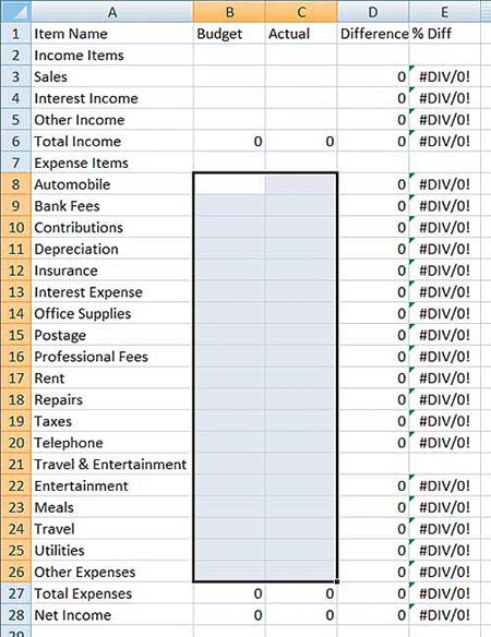
At this point, all three sheets are identical except for their names. We need to clear out the values in the February and March sheets, leaving the labels and formulas, so we can enter new values. Because the two sheets are identical and the values are in the same cells in both sheets, we can clear the values in both sheets at the same time.
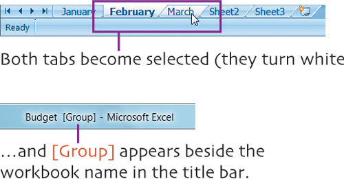
1. Click the February tab to activate that sheet.
![]()
2. Hold down the Ctrl key and click the March tab.
3. Position the mouse pointer on cell B3, press the mouse button, and drag down to cell C5 to select all of the cells with income values.

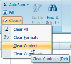
4. Choose Clear Contents from the Clear menu in the Editing group of the Ribbon’s Home tab.
The cells’ contents are removed.

5. Position the mouse pointer on cell B8, press the mouse button, and drag down to cell C26 to select all of the cells with expense values.
6. Choose Clear Contents from the Clear menu in the Editing group of the Ribbon’s Home tab (shown on previous page).
The cells’ contents are removed.
7. Click the January tab to clear the group selection. You can then click the February tab to work with just that worksheet.
insert a row
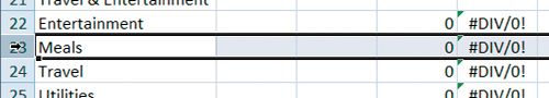
February is the month when the big company party is held. Although expenses for this party are part of Entertainment expenses, we want to track the party’s budgeted and actual expenses on a separate line. To do this, we need to insert a new row between rows 22 and 23 (Entertainment and Meals).
1. Click the February sheet tab to activate that sheet.
![]()
2. Position the mouse pointer on the row heading for row 23. It turns into an arrow pointing to the right.

3. Click once. The entire row becomes selected.
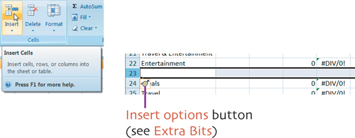
4. Click the Insert button in the Cells group on the Ribbon’s Home tab.
A new row is inserted beneath row 22 and all the rows beneath it shift down.
5. Make sure cell A23 is active—if it isn’t, click it.
6. Type Annual Party and press Enter.

delete a row
The accountant has laid down the law. No more categorizing expenses as Other Expenses. Starting in March, he wants all expenses properly categorized in one of the other existing expense categories. That means we need to delete the row for Other Expenses.
1. Click the March sheet tab to activate that sheet.
![]()
2. Position the mouse pointer on the row heading for row 26. It turns into an arrow pointing to the right.

3. Click once. The entire row becomes selected.

4. Click the Delete button in the Cells group on the Ribbon’s Home tab.

The selected row is deleted and all the rows beneath it shift up.

Have you been saving your work?
Now is a good time to click the Save button on the Quick Access toolbar to save your work up to this point.

enter new values
The February and March worksheets are ready for their values. We’ll follow the same basic steps on pages 31–32 to create entry areas and enter the data. To prevent ourselves from accidentally overwriting the formulas in cells B6 and C6, we’ll create two separate entry areas for each worksheet.
1. Click the February sheet tab to activate that sheet.
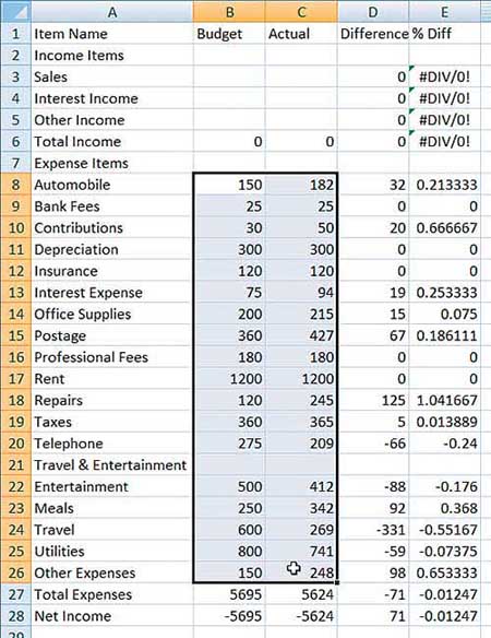
2. Drag from cell B8 to C27 to select that range of cells.

3. Hold down the Ctrl key and drag from cell B3 to C5 to add that range to the selection.

4. Enter the values shown here in each cell. Be sure to press Enter to advance from one cell to the next. Pay attention; Excel will go through the cells in the top selection before it begins activating cells in the bottom selection.

5. Click the March sheet tab to activate that sheet.
6. Repeat steps 2-4 for cells B8 to C25 and B3 to C5, entering the values shown here.

Have you been saving your work?
Now is a good time to click the Save button on the Quick Access toolbar to save your work up to this point.

extra bits
copy the sheet p. 48
• I explain how to identify the sheet tab for an active sheet on page 24.
• If you drag a sheet tab without holding down the Ctrl key, you’ll change the sheet’s position among the sheet tabs rather than copy it.
clear the values pp. 49–50
• Don’t believe that you cleared out the contents of two worksheets at once? Click the sheet tabs for February and March to see for yourself!
• It’s important to remove the group sheet selection as instructed in step 7 before entering new values in the February worksheet. Otherwise, you’ll enter the same values in both the February and March worksheets.
insert a row p. 51
• The Insert button in the Cells group inserts as many rows as you have selected above the selected row(s). So if you select three rows and click this button, Excel will insert three rows above the first selected row.
• If you select a column by clicking on its column heading, you can click the Insert button in the Cells group to insert a column to the left of it.
• The Insert Options button appears immediately after you insert a row, column, or cell. Clicking this button displays a menu of options for formatting the inserted item.

• Excel automatically rewrites formulas as necessary when you insert a row or column.
delete a row p. 52
• If you select one or more columns by clicking on or dragging over column headings, you can use the Delete button in the Cells group to delete them.
• Excel automatically rewrites formulas as necessary when you delete a row or column.
shortcut keys for this chapter
![]()