
Chapter 2
Properties
For pharmaceuticals and special fine organic chemicals, solution crystallization, in which solvents are used, is the primary method of crystallization in comparison to other crystallization techniques such as melt or supercritical crystallization. The goal of this chapter is to introduce basic properties of solution and crystals in order to better understand, design, and optimize the crystallization processes. The relevance of these basic properties to crystal qualities and crystallization operations will be highlighted accompanied with specific examples.
With regard to specific properties, we will focus on those that are more relevant to solution crystallization, and those that have direct impact on the quality of the final bulk pharmaceuticals such as purity, form, habit and size, based upon our own experience. We will leave readers to find other properties, such as miller index for crystal morphology, hardness of crystals, interfacial tension, etc. in other crystallization books (Mersmann 2001; Mullin 2001) which provide in‐depth theoretical discussion on these properties. In view of the recent development of solid dispersion, we also include relevant features of its crystallization properties. More detailed discussion of solid dispersions can be found in these references (Douroumis 2012; Shah et al. 2014; Newman 2015).
2.1 SOLUBILITY
Understanding the solubility behavior is an indispensable requirement for the successful development of crystallization processes. It is necessary to know how much solute can dissolve in the solvent system initially and how much solute will remains in the solvent at the end in order to conduct the crystallization operation. For solution crystallization, solubility of a chemical compound is simply the equilibrium (maximum) amount of this compound that can dissolve in a specific solvent system. A solution is saturated if the solute concentration is at its solubility limit. At saturation, no more dissolution will occur and the concentration of dissolved solute in the solution remains unchanged. Hence, the solid solute and dissolved solute are at equilibrium under this condition.
2.1.1 Free Energy‐Composition Phase Diagram
To deepen the understanding of thermodynamic feature of solubility, the following free energy‐composition phase diagram is presented in Figure 2.1 (Balzhiser et al. 1972, pp. 437–443).
Figure 2.1 shows the Gibbs free energy profile of a binary system, where G in the y‐axis represents the Gibbs free energy of the system, and X in the x‐axis represents the mole fraction of the desired compound. Specifically, the first component in this system can be the desired compound, and the second component can simply be the solvent. Both the temperature and pressure are maintained constant in this case.
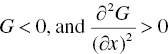
In Figure 2.1, curve‐I behaves as an upward concave curve over the entire range of composition. For this scenario, the binary mixture at any composition has a lower Gibbs free energy than two individual components. Therefore, the binary mixture at any composition is more stable than two individual components, and will become a single phase. Mathematically, the shape of concavity of this curve can be described as:
Another scenario of curve‐II contains two upward concave curves and one downward concave curve. In addition, the third curve‐III is tangent to curve‐II at points “A” and “B” of the lower part of two upward concave sections. The Gibbs free energy at points “A” and “B” can thus be expressed as a linear combination of the two intercepts of the tangent line on the Y‐axis at the composition of 0 and 1. Therefore, the intercepts of this tangent line on the y‐axis is equivalent to the partial molar Gibbs free energy of component one (the desired compound) and component two (the solvent) at composition of XA or XB. Furthermore, for component one, the partial Gibbs free energy at composition XA is identical to its partial Gibbs free energy at composition XB. This situation also applies to component two. In other words, points “A” and “B” are at equilibrium. Point “A” represents the first equilibrium (solvent with dissolved drug) phase and point “B” represents the second equilibrium oil or amorphous drug containing solvent phase. Points “A” and “B” are called the binodal points in the Free Energy—Composition diagram. The binodal points “A” and “B” can be functions of temperature and pressure. If the system’s composition lies below point A, it is undersaturated. If the system’s composition is in between points A and B, it is supersaturated. We will discuss the supersaturated condition in later Section of 2.2.1.
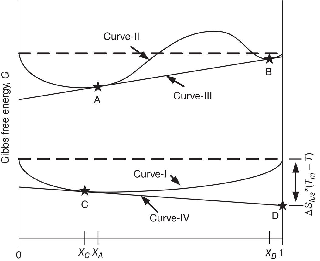
Figure 2.1 Free energy‐composition phase diagram.
Analogously, for solid–liquid equilibrium, it can be expressed as curve IV tangent to curve I at point C (equilibrium solubility) and intercepting Y‐axis at point D (equilibrium crystalline solid) for the compound of interests. Mathematically, it can be written as follows (Reid et al. 1977, pp. 380–384):

or equivalently
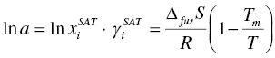
where μ is the partial molar Gibbs free energy, T is temperature, Tm is the melting point of the compound, R is the Boltzmann constant, ΔS is entropy of fusion, a is activity of compound of interests in solution, which is directly related to the amount of compound dissolved, i.e. solubility ![]() and activity coefficient
and activity coefficient ![]() In Eq. (2.2), it is assumed that the difference of heat capacities of compound as liquid and as solid is negligible. The readers can find detailed discussion on phase equilibrium of multicomponent system from the above references.
In Eq. (2.2), it is assumed that the difference of heat capacities of compound as liquid and as solid is negligible. The readers can find detailed discussion on phase equilibrium of multicomponent system from the above references.
The purpose of expressing these two equations is to show that temperature, difference of chemical potentials of compound as solid and liquid, or entropy of melting can affect directly the activity, hence the solubility. In addition, solvent, as well as impurities in the solution, can affect the activity coefficient. Chemical structure and salt forms of the compound can affect activity, entropy of melting, and activity coefficient, hence the solubility. In the following sections, we will elucidate the impact of these variables on solubility from the practical point of view.
2.1.2 Temperature
The impact of temperature on solubility is demonstrated through Figure 2.2. Figure 2.2 shows the solubility profile of lovastatin, which is a cholesterol‐lowering drug, in methanol/water mixture as a function of temperature. As shown in Figure 2.2, the solubility increases as temperature increases. This type of solubility behavior is commonly observed for organic compounds and agrees quite well with Eq. (2.2) as listed above.
In certain cases, especially inorganic salts, solubility may not be affected or actually decrease at higher temperatures. A good example is calcium carbonate water solubility (hard‐water) which has a lower solubility at higher temperatures. This reverse solubility behavior causes troublesome scale deposit issue in the hot water boiler because water is maintained at a higher temperature in the water boiler. Therefore, calcium carbonate becomes supersaturated and precipitates in the boiler. Based upon authors’ experience, however, this reverse solubility behavior is very rare for fine organics or pharmaceuticals.
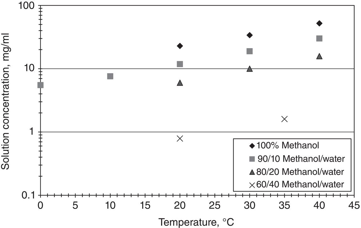
Figure 2.2 Solubility of lovastatin in different solvent mixtures as a function of temperature.
Because temperature can have such a strong influence on solubility, it is a common way in controlling the crystallization operation. The impure material can simply dissolve in a particular solvent system at an elevated temperature, and the pure material can crystallize from the solution by lowering the temperature.
2.1.3 Solvent
The solvent plays a critical role in altering the solubility as well. Figure 2.3 shows the solubility profile of lovastatin in methanol/water solvent system at room temperature. Water is used as an antisolvent for this particular example. As shown in Figure 2.3, solubility decreases sharply as water percentage increases. This is a typical solubility behavior in which solubility is reduced monotonically as antisolvent percentage increases.
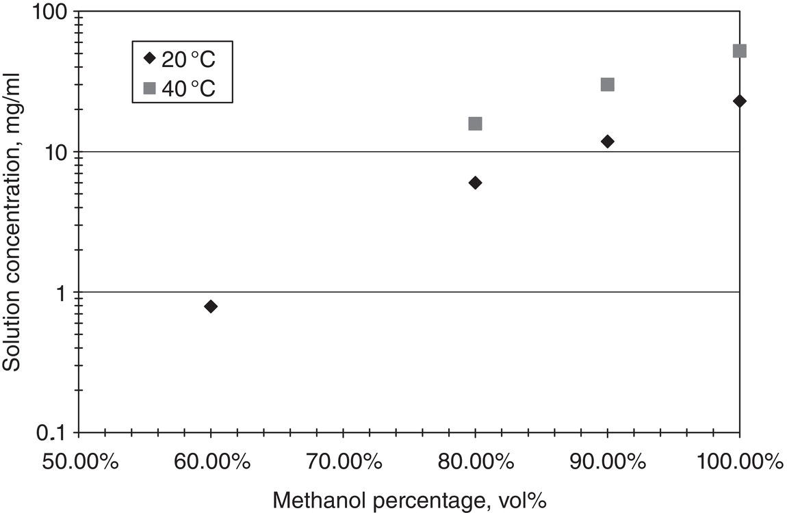
Figure 2.3 Solubility of lovastatin as a function of solvent composition.
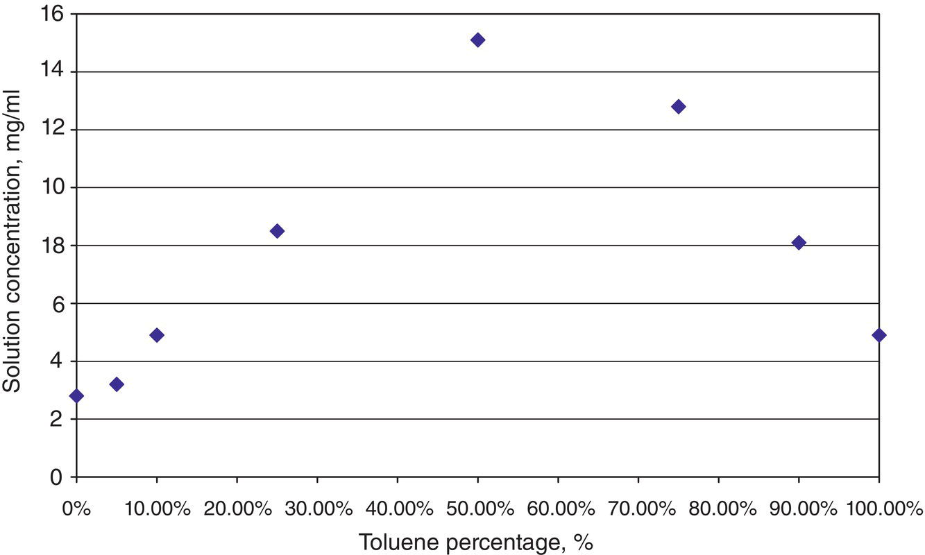
Figure 2.4 Atypical solubility behavior reaching a maximum at a certain solvent composition.
The behavior of solubility could be highly nonlinear in certain solvent systems. Figure 2.4 shows the solubility profile of a mesylate intermediate of a drug candidate in a solvent mixture of toluene/acetonitrile. Acetonitrile is used as an antisolvent for this particular example. As shown in Figure 2.4, the solubility curve reaches a maximum at the middle point of solvent mixture, and decreases at higher or lower percentages of acetonitrile. This type of behavior is less frequent than the monotonic behavior as shown in Figure 2.3, but still occurs. A simple analogy of this non‐monotonic behavior to vapor–liquid equilibrium would be the existence of (low‐boiling point) azeotrope, which has the lowest boiling point than either pure component. This reflects the impact of solvent influencing the activity coefficient of the solute and changing the solubility as shown in Eq. (2.1).
Just like temperature, the solvent composition is another common variable in controlling the crystallization process. The impure material can be dissolved in a particular solvent system, and the pure material can be crystallized from the solution by adding the antisolvent.
Solvent can strongly affect other crystallization variables, including polymorphism, solvate, crystal morphology, crystallization kinetics, etc. The impact of solvent on these variables will be addressed throughout the entire book as appropriate.
Conventional solvents, for example water, ethanol, acetone, dimethylformamide, tetrahydrofuran, isopropyl acetate, or heptane, etc. can have a wide range of hydrophilicity and hydrophobicity. Consequently, the range of solubility of an organic compound can also vary widely across the solvent landscape. In recent years, in developing the amorphous solid dispersion, different polymers with (or without) additional additives such as surfactants, are employed to “solubilize” the organic compounds. The solubility of organic compounds especially water‐insoluble drugs, in those special polymers/surfactants, for example HPMC, PVP‐VA64, or Vitamin E_TPGS, etc. could be up to 50 wt% or higher in the mixture. Clearly, those polymers/surfactants are selected with the intention to “solubilize” those water‐insoluble compounds.
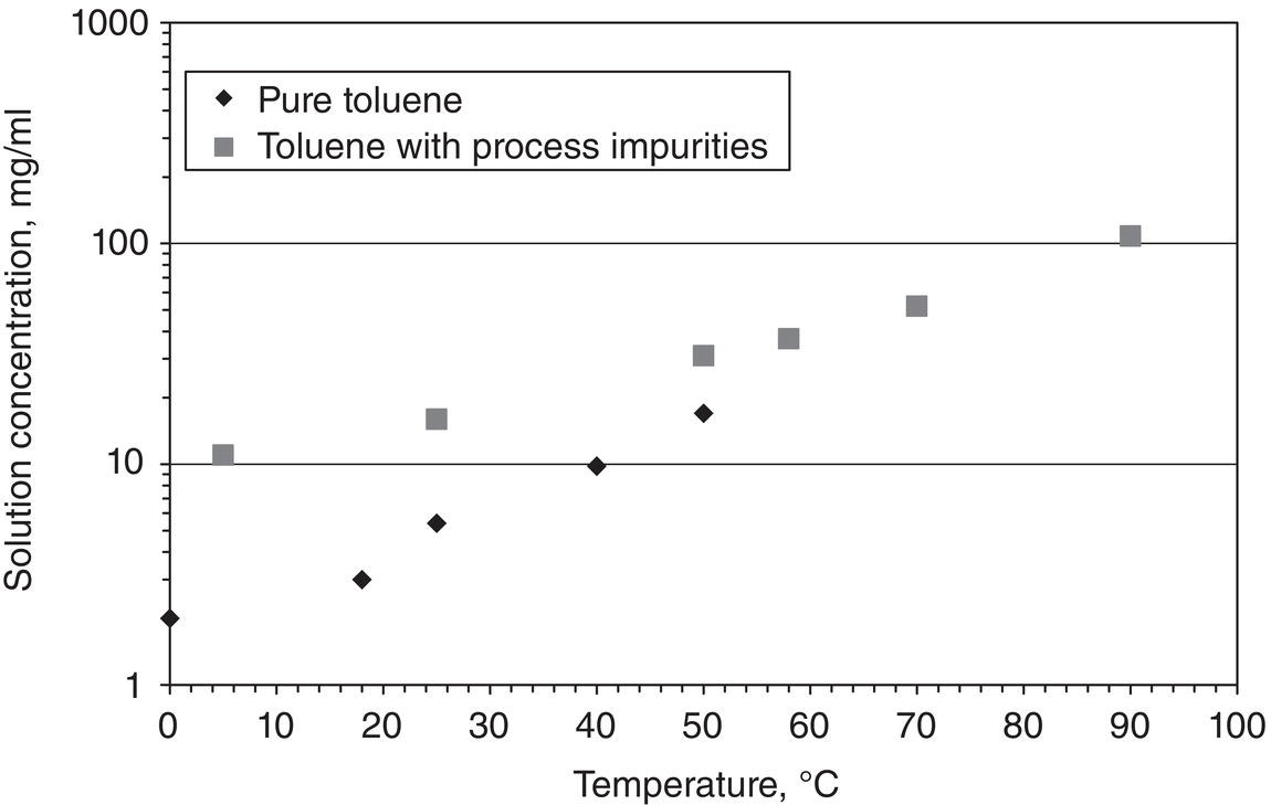
Figure 2.5 Impact of impurities on solubility.
2.1.4 Impurities
Impurities can also influence solubility to a significant extent. Figure 2.5 shows the solubility of lovastatin in pure solvent and in mother liquors. Mother liquor refers to the supernatant of the slurry after the crystallization. Mother liquor generally contains impurities rejected during the crystallization. As shown in Figure 2.5, lovastatin solubility is significantly enhanced in mother liquors than in pure solvent.
The solubility enhancement in the presence of impurities, especially in the mother liquor, is a common phenomenon. Impurities in the mother liquors may not be well characterized, albeit their chemical structures would have some degree of similarity to the desired compound. In practical applications, the impact of impurities on solubility is unknown a priori, and must be determined experimentally. Due to the potential impact of impurities on solubility, care should be taken in conducting crystallization experiments if the starting materials have varying levels of impurities from batch to batch. The presence of impurities can further affect crystallization kinetics that will be addressed in the subsequent chapter.
2.1.5 Chemical and Physical Structure, Salt and Co‐Crystal Form
If two compounds have similar chemical structures, intuitively we are inclined to assume that they would have similar solubilities. However, we should be cautious in making this assumption. Figure 2.6 shows the solubilities of lovastatin and simvastatin in methanol/water solvent system. Despite the fact that simvastatin has only one extra methyl group, their solubilities are significantly different. It is speculated that the difference is largely due to the difference of solid crystal structure of lovastatin and simvastatin, but not in the liquid phase.
It is widely known that a compound with the same chemical structure but with different physical structure of solid phase, i.e. polymorph, can have different solubilities.
If a compound contains an (or multiple) acidic or basic functional group, forming a salt can significantly alter its solubility. Needless to say, different types of salts can have quite different solubilities. Similarly, forming a co‐crystal can also significantly alter its solubility.

Figure 2.6 Impact of chemical structure on the solubility of lovastatin (compound 1) and simvastatin (compound 2) with one extra methyl group.
Since varying the salt and/or co‐crystal form can affect the solubility significantly, it is another useful technique in conducting the crystallization. For example, the desired compound may have a low solubility in the selected solvent. However, after forming the salt or co‐crystal, its solubility can increase significantly and become completely solvable. To crystallize the desired pure salt or co‐crystal, either cooling or adding anti‐solvent can be applied. Alternatively, the desired compound can dissolve in the selected solvent, and be converted to salt or co‐crystal that has a low solubility in this particular solvent. Therefore, the salt or co‐crystal will crystallize from the solution. As a matter of fact, this approach is typically called reactive crystallization. In actual practice, both approaches have been applied.
Even with the same chemical structure, it is well known that the same molecule can exist in different physical states, for example oil, amorphous solids, polymorphs, or solvates. Needless to say, different physical states generally have different solubility.
Like varying the solvent, varying the salt or co‐crystal form also affects other crystal properties including morphology, polymorphs, crystallization kinetics, formulation, drug stability, etc. Therefore, selection of salt or co‐crystal form always involves other considerations, in addition to solubility.
2.1.6 Solubility Measurement and Prediction
In the laboratory, individual solubility measurement can be performed quite easily with a simple laboratory setup. Solvent or solvent mixture and an excessive amount of solid are charged into a jacketed glass flask. The slurry is agitated and maintained at the desired temperature over a certain period, preferably overnight. Then a sample of slurry is taken and filtered through a filter. The clear filtrate is diluted for a high‐performance liquid chromatography (HPLC) assay. Generally, sampling and filtering the slurry are conducted at room temperature for ease of handling. This can introduce errors of measurement, if the temperature at which the solubility is measured is not the ambient temperature. Many modifications of this protocol are possible. For example, a filter can be incorporated into the solubility measurement glass flask so that in situ filtration can be performed.
Given the limited material supply at early phase of drug development, and the need to identify the proper solvent and temperature range for crystallization as quickly as possible, high throughput screening devices, which originated from combinatorial approach for drug discovery (Lipinski et al. 2001), are getting much wider usage. Many commercial units are currently available on the market. In general, the high throughput screening device contains multiple cells or vials in the size from microliter to milliliter range, which enable users to conduct multiple experiments with only very limited supply of materials. The key advancement of this technology really lies in automation. All operations are automated so that multiple samples can be handled repetitively (Alsenz and Kansy 2007).
Another trend in industry is the use of in situ analytical instrument, such as FTIR, Raman, ultraviolet/visible (UV/Vis), or near infrared (NIR) spectrophotometers, which are part of the process analytical technologies or PAT (Dunuwila and Berglund 1997; Podkulski 1997; Togkalidou et al. 2002). This type of instrument typically contains sensor probe which can be immersed directly into the process streams or batch. Therefore, it avoids the (offline) sampling completely and all the complications associated with sampling. In comparison to high throughput screening approach, PAT is more suitable for process monitoring, rather than analytical analysis.
Spectrophotometers can be used to measure the solubility or solution concentration. In order to establish the correlation between solubility/solution concentration and spectra peak areas, calibration with known concentrations is required. However, just like any technology, there are limitations and issues associated with in situ analytical instrumentation, such as minimum detection level, peak shift, or peak overlapping, etc. Development of an accurate correlation model for specific compounds over a wide range of temperature and solvent composition could still require a fair amount of efforts.
Measurement of organic compound solubility (or miscibility) in nontraditional polymeric matrix presents real challenges in consideration of the high viscosity of the polymer and long time to reach equilibrium below the glass transition temperature. In brief, two types of approaches are explored. The first approach is dissolution from undersaturated condition. A physical solid mixture of drug/polymers is heated until the mixture dissolves (Sun et al. 2010; Kyeremateng et al. 2014). The second approach is de‐supersaturation under supersaturated condition. A single‐phase melt or solvent‐evaporated film of drug/polymer mixture is first generated. This melt/film is then annealed at selected temperature to explore if it forms a secondary phase (Tian et al. 2013). For both approaches, modeling to extrapolate solubility and miscibility data at temperatures above glass transition temperature to room temperature is needed (Marsac et al. 2009; Suwardie et al. 2011).
Prediction of solubility is also receiving more attention. In comparison to vapor–liquid equilibrium situation which has built extensive database for reliable prediction (Reid et al. 1977), prediction of solid–liquid equilibrium remains relatively young. Noticeable progress has been made in recent years, for example NRTL‐SAC or COSMO‐SAC models (Chen and Song 2004; Tung et al. 2008b; Shu and Lin 2011).
It is worthwhile to mention the correlative and predictive natures of NRTL‐SAC model in more detail. In short, the NRTL‐SAC model is a modification of the original NRTL (Non‐Random Two‐Liquid) and polymer NRTL models for systems with oligomers and polymers. It incorporates concepts of segmental activity coefficient (SAC) by projecting the three‐dimensional electronic density function of a molecule into a one‐dimensional space containing four pre‐defined conceptual segments: hydrophobic segment (X), electrostatic polar segment (Y− and Y+), and hydrophilic segment (Z). For example, Z value for water is 1 with all other values of X, Y− and Y+ equal to 0. Likewise, X value for hexane is 1 with all other values of Y−, Y+, Z values equal to 0, and so are Y− value for dimethyl sulfoxide is ~1 and Y+ value for nitromethane is ~1.
To determine the segment numbers of a solute molecule, solubility data in four or more solvents are needed. Once the segment numbers of the solute molecule are correlated through these data, the NRTL‐SAC model can then predict the solubility in other solvents or solvent mixtures. This significantly reduces the experimental efforts and resource consumption, with reasonable confidence of the accuracy. Figures 2.7 and 2.8 show the industrial applications of NRTL‐SAC in predicting the solubilities of several compounds in different solvents. It is not a surprise that the model is able to “predict” the solubility with an excellent agreement after “correlating” the X, Y−, Y+, and Z values of solute with just few selective solvents across the segmental space.
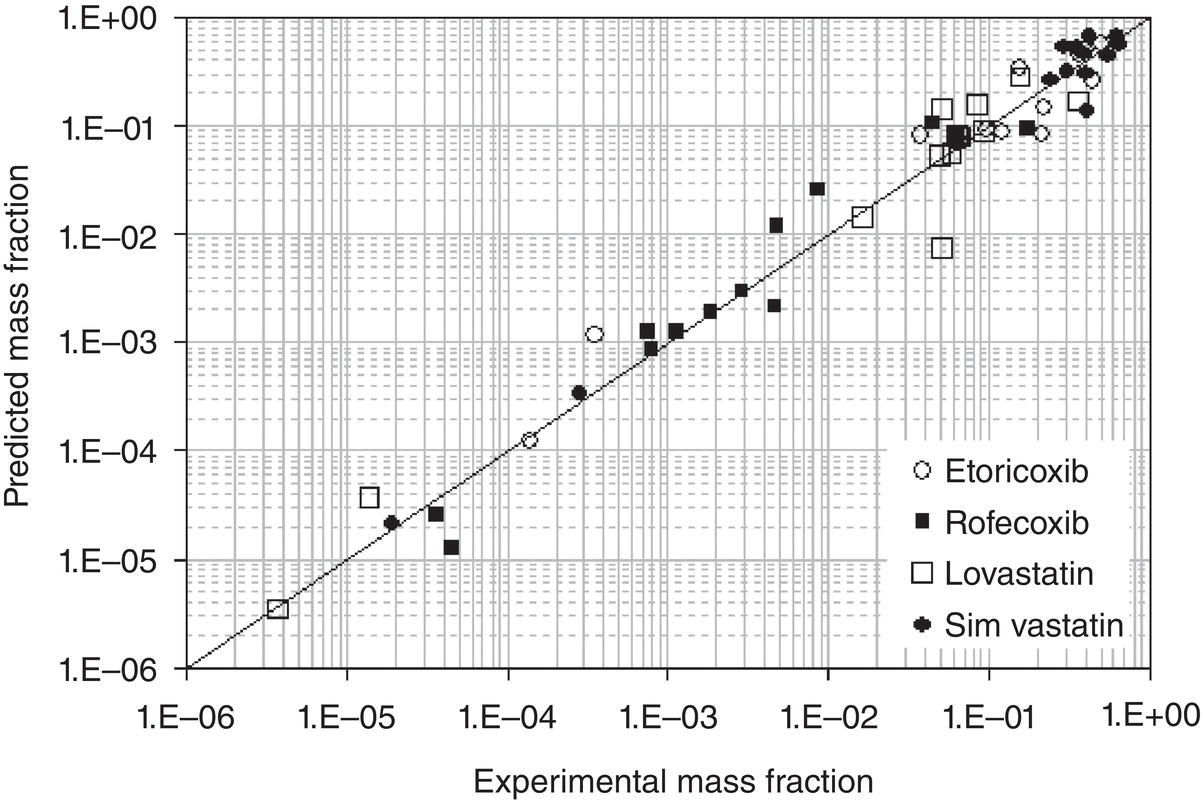
Figure 2.7 NRTL‐SAC prediction of solubility for Lovastatin Simvastatin, Etoricoxib, and Rofecoxib.
Source: Tung et al. (2008) with permission.
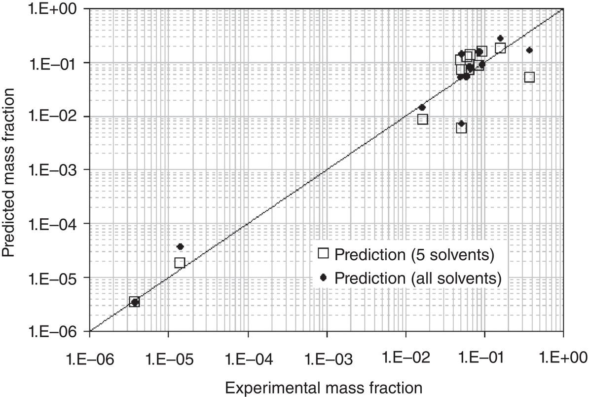
Figure 2.8 Comparison of predicted and measured Lovastatin solubility—prediction based upon 5 solvents, and correlation based upon all 13 solvents.
Source: Tung et al. (2008) with permission.
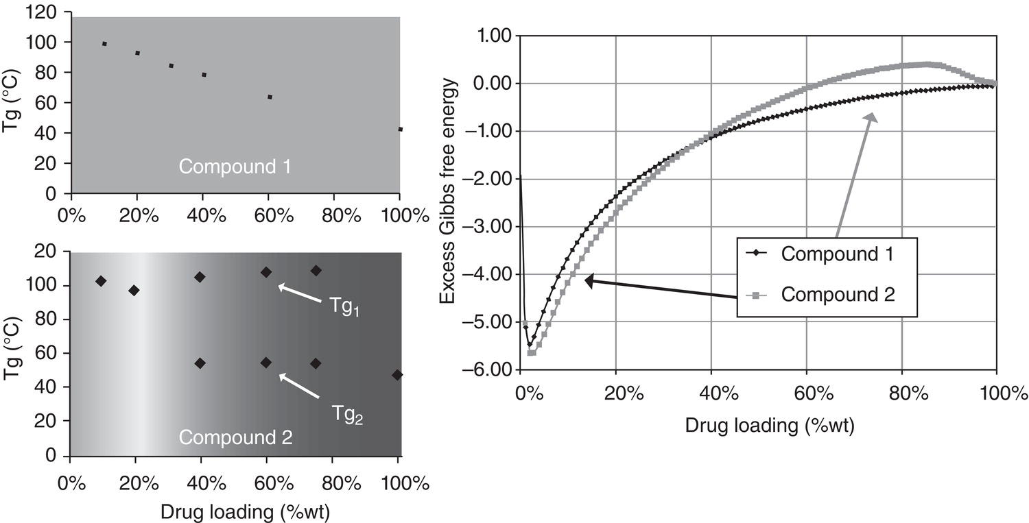
Figure 2.9 Experimental glass transition temperature (Tg) profiles (left plots) and theoretical excessive Gibbs free energy profile by NRTL‐SAC (right plot).
NRTL‐SAC can also be used to predict the solubility or miscibility of solutes in nonconventional polymeric matrix as well. Similar to the case of conventional solvents, the segmental values (X, Y−, Y+, and Z) of surfactant or polymers can be determined separately through V–L or L–L equilibrium data. Once segmental values of these polymers and surfactants are determined, the NRTL‐SAC model can predict solute solubility or miscibility in the polymeric/surfactant matrix with different combinations. The ability to “predict” the solubility/miscibility in the polymeric matrix, or even just the trend, offers a significant value to the pharmaceutical industry in screening and designing the desired solid dispersion formulation. As shown in Figure 2.9, NRTL‐SAC model shows promising results in predicting the miscibility trend of two model compounds correctly. Experimentally, for the case of compound 1, it shows only one glass transition temperature, indicating complete miscibility between the compound and the excipient. For the case of compound 2, it shows two glass transition temperatures, indicating partial miscibility, around 40% drug loading. Based upon the NRTL‐SAC approach, the calculated excess Gibbs energy for compound 1 is negative, indicating full miscibility. The calculated excess Gibbs energy for compound 2 becomes positive (around ~60 wt% drug loading), indicating immiscibility above this loading. Continuing efforts along this direction is certainly warranted.
2.1.7 Significance of Crystallization
Solubility is one key element for the development of crystallization process. As mentioned earlier, solubility allows us to determine how much solute can dissolve in the solvent system initially, how much solute will remain in the solvent at the end of crystallization, and additionally how much of each of the impurities, if their solubilities data are available, can be rejected.
Solubility ratios of the undesirable impurities over the desirable compound affects the rejection of impurity via crystallization. The higher the ratio, the better the rejection. An index of selectivity “α,” which is analogous to the situations in distillation and extraction, can be defined as
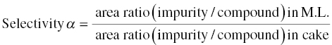
A quick approach to estimate the selectivity α is to slurry the starting material in the solvent system of choice. To facilitate the system to reach the equilibrium conditions, the slurry can be wet‐milled or sonicated during the slurry period. With some aging period, the filtrate and cake can be analyzed by HPLC. If the selectivity “α” is greater than 10, the solvent system is considered favorable.
To illustrate further, the following table presents two basic scenarios using the solubility of desired compound, impurity X, starting material purity to estimate the resulting final cake purity and yield. The purpose is to illustrate the impact of solubility on the design of crystallization process. Since it is not always possible to measure the solubility of impurities, the relationship between yield and product purity may not be determined a prior. But the general relationship between yield and product purity will still hold, i.e. the higher the yield, the lower the purity, and vice versa. Solubility data clearly provides useful information to determine the limitation of crystallization performance.
| Desired | Impurity X | Solubility ratio | |
|---|---|---|---|
| Solubility (initial condition), mg/ml | 100 | n/a | |
| Final condition, mg/ml | 10 | 10 | 1 |
| Scenario one: 85% purity, ~80 g starting material, solvent l l | |||
| Starting amount, g | 68 | 12 | |
| M.L. loss | 10 | 10 | |
| Recovery | 58 | 2 | |
| Yield | 58/68 = 85% | Selectivity | |
| Purity | 58/(58 + 2) = 97% | ~30 | |
| Scenario two: increasing starting material to 117 g, solvent 1 l | |||
| Staring amount, g | 100 | 17.65 | |
| M.L. loss | 10 | 10 | |
| Recovery | 90 | 7.65 | |
| Yield | 90/100 = 90% | Selectivity | |
| Purity | 90/(90 + 7.65) = 92% | ~12 | |
Bold values show the relationship between yield and purity, i.e. higher purity, lower yield, and vice versa.
Solubility information is also required in determining the supersaturation and crystallization kinetics. These subjects will be discussed in more details in the following sections and chapters. In addition, solubility information may be used to optimize the synthesis of drug substance and bioavailability of drug formulation. In Chapter 13 of Special Applications, the readers will find novel applications, illustrated by Examples 13.2 and 13.3 which take advantage of solubility difference between starting materials and final product to improve the reaction selectivity, overall yield, product purity, and reduction of raw material cost, and Example 13.7 which applies solubility information to design a hybrid crystalline and amorphous solid dispersion to improve drug loading, stability, and bioavailability.
2.2 SUPERSATURATION, METASTABLE ZONE, AND INDUCTION TIME
The solution is supersaturated when the solute concentration exceeds its solubility limit. A solution may maintain its supersaturation over a concentration range over a certain period without the formation of a secondary phase. This region is called the metastable zone. From the creation of supersaturation to the first appearance of the secondary phase, which is presumably solid, the time elapsed is called induction time. As supersaturation increases, the induction time is reduced. When the supersaturation reaches a certain level, the formation of secondary phase becomes “spontaneous” as soon as supersaturation is generated. This point is defined as the metastable zone width. Figure 2.10 illustrates a typical diagram of equilibrium solubility curve and metastable zone curve (Mullin 2001).
2.2.1 Free Energy‐Composition Phase Diagram
A supersaturated solution is always located beyond its solubility line; just like that a saturated solution is always located at the equilibrium line. In order to provide more fundamental insight into the metastable phenomenon, a free energy‐composition diagram, which expands further details than that shown in Figure 2.1, is presented in Figure 2.11. The readers can find more detailed discussion in the following references (Balzhiser et al. 1972; Debenedetti 1995).

Figure 2.10 Solubility and metastable zone width.
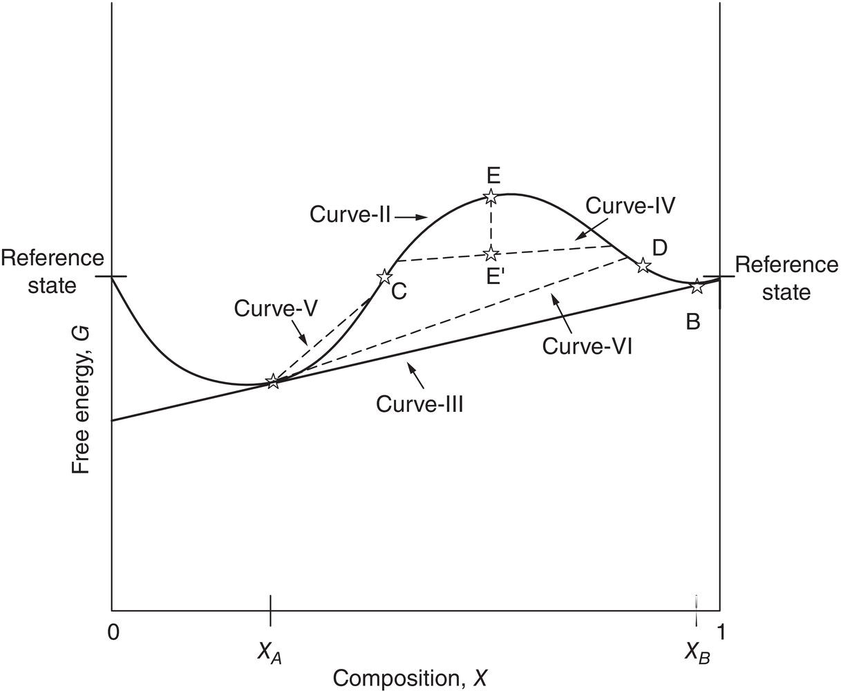
Figure 2.11 Free energy‐composition phase diagram for metastable zone region.
As mentioned in Figures 2.1 and 2.11, points “A” and “B” are equilibrium points at the lower part of two upward concave sections on curve‐II. In Figure 2.11, two additional points “C” and “D” along curve‐II are identified. These are inflection points where the upward concave curve turns into the downward concave curve. Points “C” and “D” are called the spinodal points and can be expressed mathematically as:
Spinodal points are unstable points on the free energy‐composition phase curve. For a system with composition within the region of “C” and “D,” it will spontaneously split into two phases and reaches points “A” and “B” eventually. For example, for a point “E” within this region, it can split into two phases connected through curve IV, which has the same material composition as point E. The summation of free energy of these two phases is equal to point “E,” which is “always” below the original free energy of point E. Hence the region between points “C” and “D” is unconditionally unstable. We may view spinodal point “C” as the metastable zone width of crystallization.
For any point within the metastable region, i.e. between points “A” and “C,” a small perturbation to the original state may result in a split of two phase shown as curve‐V. As shown in Figure 2.11, Curve V has a higher Gibbs free energy than the original state. Therefore, the phase split is unfavorable. The system will return to its original state and remains supersaturated. However, if there is sufficient perturbation to the system so that the phase split can cross over to the other side of free energy‐composition phase curve such as curve‐VI, the decomposition results a lower overall Gibbs free energy than the original state. For this scenario, the split is favorable. The system will release its supersaturation and the secondary phase will appear.
Clearly, depending upon the nature of the system, a supersaturated solution could have a wide range of metastable zone width. Also, the supersaturated solution may remain metastable for a long time, i.e. a long induction time, before it forms the secondary phase, which may exist as oil, amorphous, or crystalline solid.
2.2.2 Factors Affecting Metastable Zone Width and Induction Time
Similar to solubility, metastable zone width and induction time of a supersaturated solution are affected by various factors, including temperature, solvent composition, chemical/physical structure, salt/co‐crystal form, and impurities in the solution, etc. Therefore, although spinodal point is considered to be a thermodynamic property, it is very difficult to measure the absolute value for metastable zone width experimentally. Regardless, understanding the qualitative behavior of metastable zone width and induction time can be helpful for the design of crystallization processes.
From the point of view of free energy‐composition phase diagram, it is reasonable to expect that distance between the spinodal and binodal points should become smaller as temperature of the system increases, provided there are no additional complications such as thermal or chemical decomposition. This expectation is based upon the assumption that at sufficiently high temperatures two phases will mix freely with each other (assuming totally miscibility). Therefore, the system becomes a single phase, i.e. curve II converges to curve I or points “A” and “B” moves closer and merge with each other as shown in Figure 2.1. If it happens, it means equivalently that the metastable zone also becomes narrower and induction time is shorter at higher temperatures. Broadly speaking, this assumption is consistent with the authors’ experience for the case of cooling crystallization. For the case of antisolvent or reactive crystallization, it seems reasonable to expect that metastable zone width will be narrower and induction time will be shorter at a lower level of antisolvent level. However, more data are needed to substantiate this hypothesis. As mentioned earlier in Section 2.1.3 of solvent impact on solubility, there could be many exceptions to this hypothesis. As to the impact of impurities, the higher the level of impurities in the solution, the broader and longer the metastable zone and induction time.
Other factors, such as presence of seed of desired compound, undissolved extraneous solid particles, and needless to say mixing intensity or local turbulence etc. can affect the metastable zone width and induction time. Clearly, these factors can perturb and alter the local free energy‐composition phase curve at the microscopic scale. In general, these factors will lower the metastable zone width, and also reduce the induction time.
2.2.3 Measurement and Prediction
Determination of solution concentration, either at supersaturated or saturated states, can be performed offline by taking slurry samples from the process, similar to the measurement of solubility in Section 2.1.6. This method suffers complications due to temperature variation and solvent evaporation. In addition, sampling is generally time and labor intensive. As mentioned earlier, in situ analytical instrument such as FT‐IR or UV‐visible spectrophotometer can measure the solution concentration and calculate the supersaturation given the solubility information. Accurate determination of supersaturation can greatly assist the understanding of crystallization kinetics and the development of crystallization process.
Reliable determination of metastable zone width and induction time generally is more time consuming and difficult than the determination of supersaturation. This is because metastable zone width and induction time are affected by various factors. Therefore, the data may not be reproducible when the operating environment is changed. On the other hand, accurate measurement of metastable zone width or induction time is not critical for many industrial applications. A few data points for rough estimation are generally sufficient for the design of crystallization processes. On the contrary, metastable zone width or induction time has critical impact for amorphous solid dispersion. If drug is supersaturated and phase‐separated within the dispersion, it will inevitably impact dissolution and bioavailability.
To measure the metastable zone width, the first step is to prepare a slightly undersaturated solution based upon solubility data. For the case of cooling crystallization, the clear undersaturated solution is cooled at a finite rate to generate the supersaturation. During the cooling, the solution becomes cloudy and marks the boundary of metastable zone at this particular cooling rate. Since cooling rate can affect the measured metastable zone width, this procedure may need to be repeated several times using different cooling rates. The asymptotic point with zero cooling rate defines the ultimate “true” metastable point. To construct the entire metastable zone width curve, this approach will be repeated at different initial solution concentrations. For the case of antisolvent crystallization, similar protocols can be developed to measure the metastable zone width. The procedure for measuring the metastable zone width can be facilitated by using an in situ particle size analyzer, such as focused beam reflectance measurement (FBRM) device that can detect and measure the particle size without sampling for external analysis (Birch et al. 2005). Experimental determination of metastable zone width or induction time for (amorphous) solid dispersion is nontrivial or essentially nonexistent, in consideration of the high viscosity of the polymer and long time to reach equilibrium below the glass transition temperature. For ensuring suitable shelf life stability, a short‐term one‐ to three‐month study coupled with long‐term one to two years study are required.
From the discussion of solubility above, it is theoretically possible to deduct the metastable zone width through the free energy‐composition curve, if such a curve is available (Kim and Mersmann 2001). Due to the complexity of the problem, experimental verification is preferred for practical applications.
2.2.4 Significance of Crystallization
The ability to generate supersaturation is a necessary requirement for conducting crystallization. As inferred from Section 2.1 of solubility, supersaturation can be created by varying the temperature, solvent composition, and its salt form. Practical cases based upon the method of generation of supersaturation will be presented in details from Chapters 7–Chapter 10 in this book.
In general, for batch crystallization with a narrower metastable zone width, the operating window for generation of supersaturation is smaller. It is more likely to create nucleation with fine crystals, and vice versa.
It is not always desirable to have a wide metastable zone width, though. Figure 2.12 shows the concentration profile of a tartrate salt during the course of crystallization. The tartrate salt was formed by the addition of L-tartaric acid to a solution of free base in a solvent mixture of acetonitrile/ethyl acetate/water. As shown in Figure 2.12, the solution remains highly supersaturated (metastable) over an extended period after the addition of tartaric acid to the free base, if the seed surface area is not sufficiently high. Increasing the seed surface significantly facilitates the release of supersaturation.
The presence of highly supersaturated metastable solution, coupled with a slow release of supersaturation, can be problematic. First, slow release of supersaturation will significantly lengthen the batch time cycle. Second, the highly supersaturated solution may lead to unpredictable nucleation which would be difficult to control and create inconsistent performance from laboratory to factory and from batch to batch.
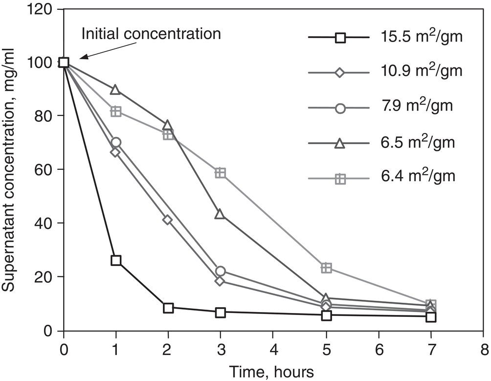
Figure 2.12 Solution concentration profile during crystallization.
There are also cases that tentatively exceed the metastable zone width during the crystallization, for instance impinging jet crystallization shown in Examples 9.5 and 9.6. Since the induction time becomes extremely short, the final product size depends strongly on the distribution of local supersaturation. Successful process design to obtain consistent Particle Size Distribution (PSD) will require tight control of mixing and generation of supersaturation. As mentioned, a detailed description of the impinging jet crystallization is given in Examples 9.5 and 9.6.
Metastability and induction time can play an interesting role for the kinetic resolution of optical isomers, such as Example 7.4 of resolution of ibuprofen lysinate. On the one hand, in order to maintain the optical purity of the desired isomer, it is necessary to keep the “undesirable” isomer in its supersaturated state for the entire crystallization period. If the undesired isomer crystallizes out from the solution, the optical purity of the desired isomer will decrease. On the other hand, it is desirable to release the supersaturation of desired isomer which starts at the same initial level of supersaturation as the undesirable isomer. Therefore, these are two conflicting requirements. To overcome this dilemma, it is critical to maintain a large amount of seed bed of the desired isomer to accelerate the release of supersaturation of the desired isomer, whereas the undesired isomer remains supersaturated. As mentioned, a detailed description of the resolution process of optical isomers is given in Example 7.4.
For the application of solid dispersion, the metastable supersaturated state can impact not only the drug’s shelf life, but also its dissolution and bioavailability in vivo. It remains an active research topic (Moseson et al. 2021).
2.3 OIL, AMORPHOUS, AND CRYSTALLINE STATES
Upon release of supersaturation, the initially dissolved compound will be separated from the solution and form a secondary phase, which could be either oil, amorphous solid, or crystalline solid. Crystalline materials are solids in which molecules are arranged in a periodical three‐dimensional pattern. Amorphous materials are solids in which molecules do not have periodical three‐dimensional pattern. Under some circumstances with very high supersaturation, the initial secondary phase could be a liquid phase, i.e. “oil,” in which molecules could be just “randomly” arranged in three dimensional patterns and have a much higher mobility than solids. Generally, the oil phase is unstable and will convert to amorphous material and/or crystalline solid over time. At a lower degree of supersaturation, amorphous solid can be generated. Similar to the oil phase, the amorphous solid is unstable and can transform into crystalline solid over time. Even as crystalline solid, there could be different solid states with different crystal structure and stability. The formation of different crystalline solid state is the key subject of polymorphism that will be mentioned below and further in more detail in Chapter 3. The transformation from the unstable states to stable states is generally called Ostwald rule of stage effect (Mullin 2001).
The oil, amorphous, and crystalline states of materials are phenomena frequently encountered during the crystallization. In the following discussion, we will try to exemplify these phenomena based upon its dependence on supersaturation.
2.3.1 Phase Diagram
Figure 2.13 shows a diagram that outlines the relationship of oil, amorphous material, and crystalline material with respect to supersaturation. We should emphasize that this diagram is primarily based upon empirical observation over years of development of crystallization with various compounds. There is no intention to build a theoretical framework through this diagram. In comparison to metastable zone width, there is relatively little discussion on the “oiling” phenomenon in the literature (Bonnet et al. 2002; Lafferrere et al. 2002; Davey et al. 2013). Therefore, it is beneficial to present such a diagram even without much theoretical derivation.
As shown in Figure 2.13, when an extremely high supersaturated solution is created, it can form a secondary oil (and/or gel) phase initially. As an example, Figure 2.14 shows the appearance of oil droplets in a highly supersaturated simvastatin solution. In this example, the secondary phase of oil droplets was observed initially after mixing a clear concentrated batch solution with enough antisolvent instantaneously to form a highly supersaturated solution. The resulting oil droplets are unstable and quickly transformed into small crystalline solid upon aging. It has also been observed for other compounds that the oil droplets convert to amorphous solids upon aging.
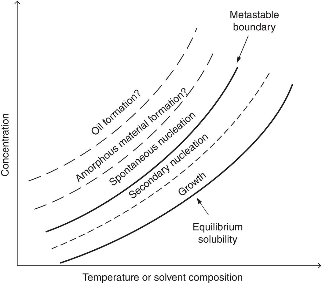
Figure 2.13 Expanded map on metastable zone width.
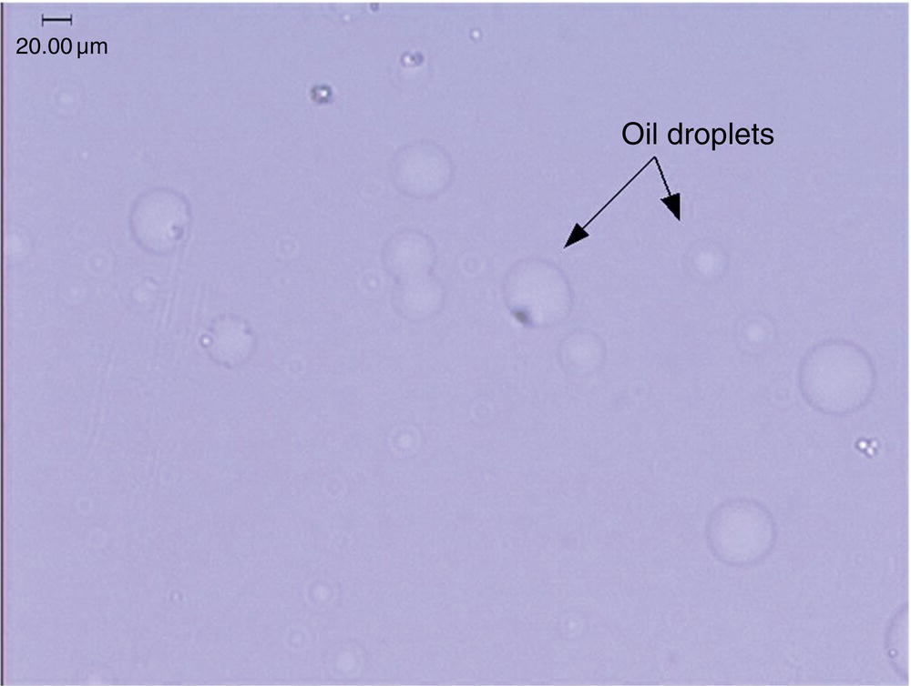
Figure 2.14 Formation of oil droplets of a highly supersaturated solution.
For a less supersaturated solution, Figure 2.15 indicates that the amorphous solid can be generated after aging the oil droplets. Another example of forming the amorphous solid can be accomplished by rapid cooling of a saturated solution as encountered in lyophilization or freeze‐drying operations. Similar to oil droplets, amorphous solid is unstable and will transform into crystalline material upon aging at proper conditions. As shown in Example 13.5, the amorphous imipenem can be transformed into crystalline material even at freezing condition.

Figure 2.15 Formation of amorphous solid after aging of oil droplets.
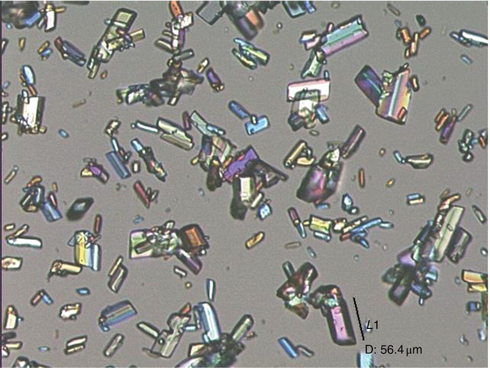
Figure 2.16 Formation of crystalline solid.
The most stable and desirable solid phase upon release of supersaturation is clearly a crystalline solid as shown in Figure 2.16. A crystalline solid is generally purer and more stable than amorphous solid and oil droplets. The majority of organic chemicals, especially pharmaceuticals, are produced as crystalline solid.
We should point out that in practice, we may not always observe all three different forms of state. For the case of simvastatin as shown in Figure 2.14, under the microscope, the oil droplets seem to convert directly to crystalline solid without the intermediate amorphous solid. For some materials, we have never observed the formation of oil droplets under the conditions of crystallization. However, the generality of this phase diagram appear to be valid crossing over a wide range of compounds, and have been proven useful in guiding us through the development of crystallization.
It would be interesting to explore some variants of the phase behavior. One variant would be solid dispersion. A hypothetic phase diagram, based upon the one proposed by Qian et al. (2010a), is presented in Figure 2.17a to illustrate the relationship among the solubility, miscibility and Tg curves behavior of drug and amorphous polymer/excipient. In regions I and II, the drug concentration is below its solubility curve in excipient. Therefore, the drug/excipient composite is physically stable. In regions III, IV, V, and VI, the drug level exceeds the solubility limit. Therefore, the composite is metastable and the excess amount of drug can convert to stable crystalline solid. Furthermore, in regions V and VI, the drug level is above the miscibility curve. The miscible curve resembles the oil formation curve in Figure 2.13. Above the miscibility curve in regions V and VI, the system can split into two immiscible amorphous phases. These two immiscible amorphous phases remain metastable and can convert to the corresponding stable crystalline drug material and amorphous polymeric phase over time. The formation of two immiscible amorphous phases can be detected by the presence of two distinct Tg values during differential scanning calorimetric analysis. This scenario is highlighted in the model compound 2 as shown in Figure 2.9. The immiscibility curve may not exist for other compounds. This scenario is shown in the model compound 1 in Figure 2.9.
The kinetic of crystallization in regions III, IV, V, and VI can vary widely from compounds to compounds. It is possible that the phase separation kinetics is faster in regions VI (and IV) which are above the Tg curve, and is slower in regions V (and III) which are below the Tg curve.

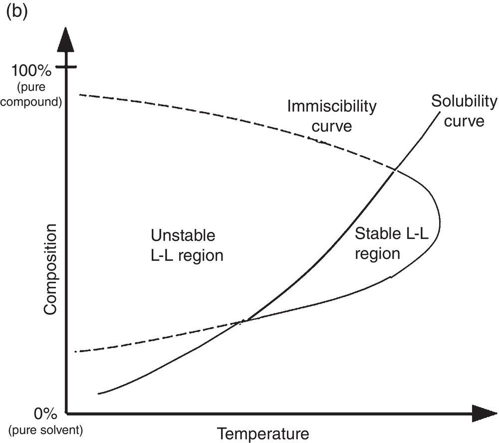

Figure 2.17 (a) Solubility, miscibility, and Tg curves of solid dispersion. (b) Solubility and miscibility crossover. (c) Crystalline solids convert to oil droplet upon heating.
Another variant of the phase behavior is the relative location of immiscible oil phase or L–L phase versus the crystalline solubility or solid–liquid (S–L) phase. In less common cases, the L–L phase becomes the stable equilibrium phase and the S–L phase becomes the metastable solid phase. As shown in Figure 2.17b, the L–L immiscibility curve can cross over the S–L solubility curve and become the stable phase. This phenomena is vividly illustrated in Figure 2.17c. Under the microscope, a crystalline solid with a melting point greater than 100°C is slurred in MeOH/water ½ system. At ambient temperature, it forms a typical S–L phase. Upon heating (>43°C), crystalline solid converts to oil droplets and forms L–L phase. Another reported example of this type phase behavior is racemic ibuprofen in ethanol water system (Rashid et al. 2014).
2.3.2 Measurement
Oil, amorphous, or crystalline materials can be easily distinguished under the microscope. Oil is simply a secondary liquid phase. Amorphous material generally has no definitive shape without any birefringence under the polarized light. Crystalline materials typically have a defined shape or interfacial angles between faces, and will show birefringence under polarized light (Stoiber and Morse 1994). The detection limit of particle size by optical microscope is close to 400 nm which is at the boundary of visible light wavelength. Therefore, any oil or solid particle of less than 400 nm size would not be observable under the optical microscope. This imposes a concern on the detectability of residual crystalline drug nanoparticles in amorphous solid dispersion through optical microscope.
For more quantitative measurement, X‐ray powder diffraction analysis is commonly used in industry (Hancock and Zografi 1997; Jenkins 2000). A crystalline solid will typically show several distinct peaks which reflect the unique structure of crystals, whereas amorphous solid will not have any distinct peaks. This technique could be further used to assess quantitatively the degree of amorphism within a solid as mentioned in Example 12.5 (Connolly et al. 1996). For this particular case, it is demonstrated that the shift of baseline of X‐ray diffraction spectra is proportional to the degree of amorphism in the solid phase (Crocker and McCauley 1995). While this method can be quantitative, the detection limit of residual crystalline drug within the amorphous material generally lies in between 1 and 5% which is less sensitive than that of optical microscope.
Another frequently applied technique is differential scanning calorimetry. By heating a solid sample at a preselected heating rate, the resulting heat flow profile over temperature can reveal the degree of crystallinity of the solid sample. For 100% crystalline solid, this solid should only melt at or near its melting point. Therefore, the heat flow profile should be smooth over the entire heating period and will only detect an endothermic heat flow corresponding to enthalpy of melting at its melting point. If there is some degree of amorphous solid present in the solid, it is likely to observe some degree of solid‐state transition and corresponding heat flow prior to melting. In the study of simvastatin, it is shown that the differential scanning calorimetry can effectively measure the melting point depression and can be applied to differentiate defect of crystals generated by several different crystallization methods (Elder 1988, 1990). The correlation between the melting point depression and other quality variables, such as amount of polymer dissolved or impurities in the crystalline drug during heating, can be quite useful for quick ranking or quantitative assessment. On the other hand, detection of residual crystallinity in amorphous material can be more challenging due to the possible thermal relaxation of amorphous state to crystalline state upon heating. It is shown that two amorphous solid dispersion samples with identical differential scanning calorimetric profiles exhibit different level of recrystallization of drug over time (Qian et al. 2010b).
2.3.3 Significance to Crystallization
The oil droplets generally contain very high level of impurities that include solvents, and create very difficult purification problem. In addition, the oil phase is essentially a liquid phase, and simply cannot be isolated as solid for further drug formulation work. The oil phase is unstable and will likely convert into amorphous or crystalline solid upon aging, but without much control of final particle size. Therefore, the formation of oil phase becomes an obstacle for the process. Seeding and control of supersaturation are common techniques to overcome this difficulty (Deneau and Steele 2005). Amorphous material has similar complications of impurity rejection and solid state instability as the oil material. Therefore, the formation of amorphous solid is generally undesirable, although sometimes some compounds cannot or are difficult to form crystalline solid. Certain drugs, for example for those that are produced via freeze drying, are inherently amorphous solids. These amorphous drugs are made primarily to improve its dissolution rate into human body, but at the expense of drug stability and sub‐ambient storage temperature (Leuner and Dressman 2000). Amorphous solid dispersion is another technique to generate amorphous solid to increase the bioavailability. Similarly, amorphous solid dispersion can face the issue of potential recrystallization over time if the drug loading exceeds the solubility/miscibility limit. By far, crystalline solid remains the most desirable form for drug substance and drug formulation, although more attention is being given to amorphous solid dispersion (Lowinger et al. 2007).
A more detailed discussion on the impact of phase diagram on the process development of crystallization is given in Chapter 6—Critical Issues.
Maintaining the crystallinity is required not just during the crystallization, but also in the subsequent steps such as the filtration, drying, and milling. For a hygroscopic solid, the solid will absorb water and may lose its crystallinity (see Section 2.9). For solvates or hydrates, desolvation or dehydration during drying can generate amorphous desolvates or anhydrous materials. Therefore, controlling the drying and storage humidity will be critical for this type of materials. For some crystalline materials, it may have the tendency to lose its crystallinity under drying (heat) or milling (pressure). Special attention will be required in order to maintain the crystallinity.
2.4 POLYMORPHISM
A compound may form crystalline solids which have more than different three‐dimensional structures. This results in polymorphs (Brittan 1999). With this definition, all polymorphic crystals should be the same molecular species, but with different crystal structures. Please note that optical isomers, which have the same chemical structure, are considered to be different molecular species and should not be confused with polymorphism. Only a brief description of this subject is mentioned below. A more detailed discussion is given in Chapter 3.

Figure 2.18 Solubility curves of monotropic and enantiotropic polymorphs.
2.4.1 Phase Diagram
Polymorphism crystals typically exhibit different physical properties and behaviors, such as solubility and melting point. Figure 2.18 shows solubility curves of monotropic and enantiotropic polymorphs. For the monotropic polymorphs, polymorph I has a lower solubility than that of polymorph II throughout the entire solubility range. For the enantiotropic polymorphs, polymorph I has a higher solubility than that of polymorph III at the lower part of solubility range, but has a lower solubility than that of polymorph III at the higher part of solubility range, or vice versa.
Polymorphism is a common phenomenon in chemical and pharmaceutical industries. For example, Figures 2.19 illustrates the solubility of form I and III polymorphs of a reverse transcriptase inhibitor drug candidate which exhibit enantiotropic behavior. Also, Figure 2.20 shows the microscopic photos of transformation of form III crystals to form I crystals after aging.
As shown in Figures 2.19, the unstable form, i.e. form III, could be generated at higher supersaturations. As shown in Figure 2.20, once generated, the unstable form III is then converted into a stable form, i.e. form I.
2.4.2 Measurement and Prediction
Identification of polymorphism is ultimately based upon on X‐ray powder diffraction pattern analysis. Two forms of crystal must have two different diffraction patterns. Polymorphs will also have different melting points, spectroscopic patterns, and differential scanning calorimetric profiles (Giron 2000; Class 2003). Microscopic examination of crystal morphology can be a quick method as well, as long as polymorphs have distinct difference in morphology or shape as shown in Figure 2.20. One interesting work is the identification of the specific crystal form via the 3D‐crystal morphology of a crystal (Singh et al. 2012). The 3D‐crystal morphology is constructed through multiple 2D‐crystal images at different focal depth. After constructing the 3D‐crystal morphology of the crystal, the angular patterns among all crystal surfaces on the crystal are calculated and compared to the angular patterns of all known crystal forms of the compound. Since each crystal form has its own unique angular patterns, this method can identify the specific crystal form based upon simply the crystal morphology. The correlation between crystal form and morphology using microscope could offer potential advantages over other established techniques such as Raman or powder X‐ray diffraction method, such as simplicity of measurement, a significant reduction of equipment and maintenance cost, and a better sensitivity in detecting crystals of undesired forms within the matrix of crystals of desired form.
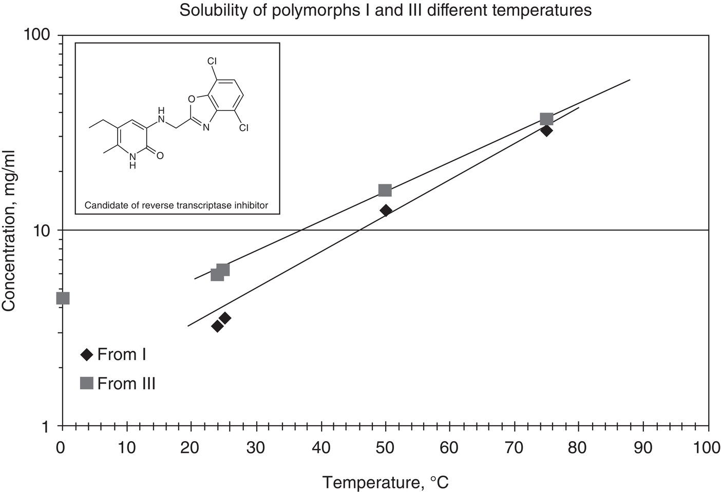
Figure 2.19 Solubility of form I and III polymorphs of a reverse transcriptase inhibitor.

Figure 2.20 Conversion of forms I and III mixture to form I after aging.
Polymorphs generally have different solubilities, which can also assist in identifying the stability of polymorph as shown in Figure 2.18.
In situ determination of polymorphism is via PAT (e.g. O'Sullivan and Glennon 2006; Chianese and Kramer 2012), as mentioned in Section 2.1.6.
Numerous publications on the prediction of polymorphs are appearing each year, reflecting the level of interest on and importance of this field, for example Myerson (1999), Vippagunta et al. (2001), Neumann et al. (2008), Kendrick et al. (2011), Price (2014), Pantelides et al. (2014), Hilfiker and Raumer (2018), Li and Mattei (2018), etc. The approach is primarily based upon the minimization of crystal lattice energy of various molecular orientations, in particular through the propensity of molecular hydrogen bonding among molecules. Besides the thermodynamic equilibrium approach, an alternative approach is to predict the formation of polymorphs through the kinetic pathway, i.e. nucleation rates of selected polymorphs (Chen and Trout 2008; Davey et al. 2013; Parks et al. 2017). In this approach, the nucleation rate is expressed as a function of excessive Gibbs’ free energy and associated rate constant, which are computed through Monte Carlo simulation. Further discussion and case studies will be presented in Chapter 3.
Computational approaches seem to predict both “non‐feasible” polymorphs and “feasible” polymorphs. On the other hand, experimental screening may not discover all the feasible polymorphs. Incorporating the kinetic factor (Parks et al. 2017) into the polymorph screening and through authors’ experience, discovering of all feasible polymorphs appears to be feasible in the near future.
Nevertheless, in silico prediction of polymorphs can be very helpful and complimentary to the experimental works, just like the in silico prediction of solubility.
2.4.3 Significance to Crystallization and Downstream Operations
Crystal form can be considered to be the most critical physical attributes for pharmaceuticals. Crystal form affects bioavailability, drug stability, and formulation process operability. The criticality of discovering the most stable, if not all, polymorphs of the drug substance at the early stage of drug development is far beyond crystallization. If a more stable form is discovered in the late phase of drug development, all previous developmental results, including crystallization of pure bulk, need to be reevaluated. For the same reason, if the stable form is discovered after the drug is marketed, the impact can be much more dramatic. Fortunately, the latter scenario only happened once in a while (Rouhi 2003).
In the presence of polymorphs, developing a proper crystallization process to control the desired crystal form is a real challenge. A good understanding of solid–liquid equilibrium behaviors under different conditions, for example temperature or solvent mixture, is a must. Seeding and control of supersaturation are two very critical, if not indispensable, requirements. Example 7.5 shows an example of developing a crystallization process of a polymorphic compound.
Just like the solid crystallinity topic as mentioned in Section 2.3.3, it will not be sufficient only to grow the desired polymorphs during the crystallization. It is required to maintain the desired polymorphs throughout the entire operation sequence such as filtration, drying, and milling. For the enantiotrophic system, turning over from a polymorphic form which is stable at room temperature to another polymorphic form which is stable at a higher temperature, may occur if the drying temperature is above the crossover temperature. Clearly it would be desirable to maintain the drying temperature below the crossover temperature.
2.5 SOLVATE
As the name indicates, a compound can incorporate solvent into its crystal lattice and forms a different crystal, just like the case of polymorphism. However, solvate and original non‐solvate material are not identical chemically due to the presence of solvent. Therefore, they are really two different compounds. In practice, almost all solvates found are crystalline material, while the “anhydrous” material could be either amorphous or crystalline solid.
2.5.1 Phase Diagram
Similar to polymorph materials, non‐solvate material and solvate exhibit different physical properties and behaviors. Figure 2.21 shows solubility curves of typical non‐solvate and solvate solids as a function of solvent composition and temperatures. As shown in Figure 2.21, the non‐solvate solid and solvate solid cross over at composition “A1.” Above composition A1 solvate solid has a lower solubility (shown as solid line) than non‐solvate (shown as dotted line), and is more stable. Similarly below composition A1 non‐solvate solid has a lower solubility than solvate, and is more stable. The crossover points A1–A3 forms the crossover line that is a function of temperature. In general, the solvent composition of crossover point increases as temperature increases.
Solvated crystals are also a common phenomenon in the chemical and pharmaceutical industries. Figure 2.22 shows the room temperature solubility curve of ibuprofen‐lysinate as a function of water content in ethanol. As shown in Figure 2.22, the crossover point between anhydrous solid and monohydrate is ~5% water level. At room temperature, ibuprofen‐lysinate remains anhydrous when the water content is below 5%, and transforms to monohydrate when the water content is above 5%. For this particular example, solvate and anhydrous material also have different crystal habit as shown in Figure 2.23.
A particular case of solvate is hydrate of which water molecules form a solid adduct to the parent compound. Hydrate may not be stable below a certain water level, and may lose its water molecule and form the anhydrous crystalline or amorphous solids. Above the crossover water level, hydrate is stable and always has a lower solubility than the solubility of anhydrous solid (Khankari and Grant 1995).
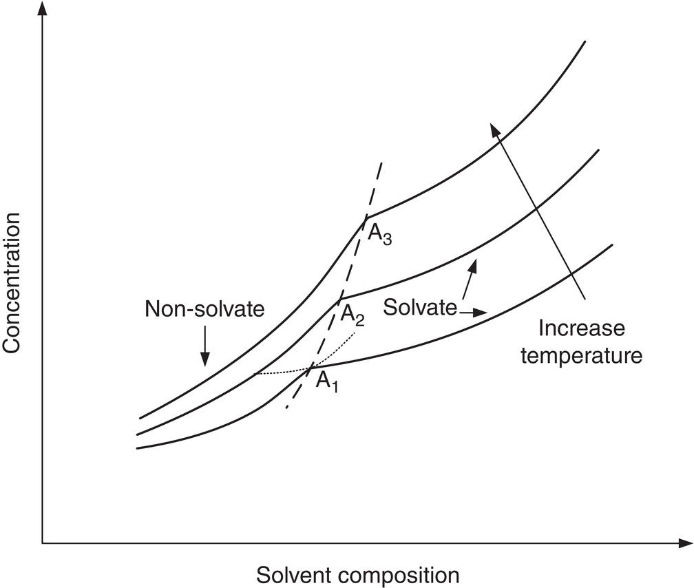
Figure 2.21 Solubility diagram of solvate and non‐solvate at different temperatures.
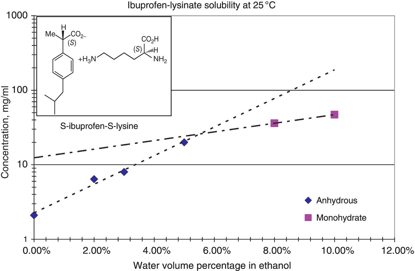
Figure 2.22 Solubility of anhydrous solid and monohydrate of ibuprofen lysinate.
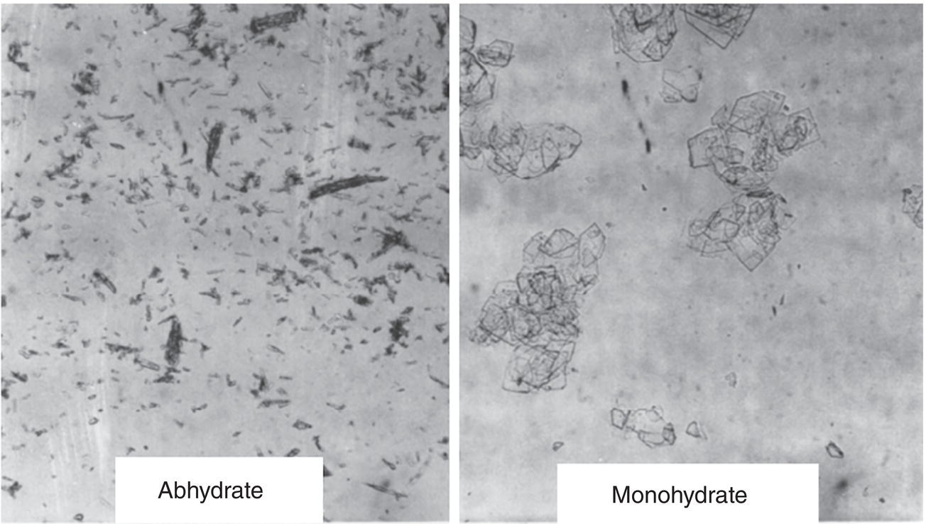
Figure 2.23 Anhydrate versus monohydrate crystals of ibuprofen‐lysinate.
2.5.2 Measurement and Prediction
Essentially, all analytical tools mentioned in Section 2.4.2 are applicable for the measurement of non‐solvate and solvate. In addition, the presence of solvent in a solvate can be confirmed by GC‐mass analysis of the solid.
Special attention should be given in preparing the sample to avoid the solid state transition from solvate to non‐solvate. It is not uncommon to observe that the wet cake solvate loses its solvent during drying. The dry cake becomes non‐solvated solid which is no longer the true solvate solid in the crystallization.
Prediction of solvate or hydrate structure is generally considered within the framework of polymorph prediction. Please see Section 2.4.2.
2.5.3 Significance to Crystallization and Downstream Operations
Similar to polymorphism, the presence of solvate can present a challenge for the drug development beyond crystallization (Variankaval et al. 2007). It is crucial to have a good description of equilibrium solubility behaviors under different operation conditions. Seeding and control of supersaturation are also required to successfully control the crystallization process. Example 7.5 will present an example on the development of crystallization process for producing the correct polymorph.
As mentioned above, special attention should be given in drying operation of the wet cake. It is not uncommon that the wet cake solvate loses its solvent during drying, and turns into non‐solvate solid that can be either desirable or undesirable. For the particular case of hydrate, it is generally required to maintain the proper humidity in the vapor phase during drying and storage in order to maintain its hydrate form.
2.6 SOLID COMPOUND, SOLID SOLUTION, AND SOLID MIXTURE
When a compound incorporates a second compound other than solvent into its crystal lattice, it creates a new material called solid compound. Salts and co‐crystals are thus considered to be in this category. As the name implies, solid compound and solvate are similar phenomena. Just like solvate, the ratio of the first compound to the second compound in the solid crystal lattice is fixed. However in certain cases, the ratio can vary over a certain range. For this scenario, the new compound is called solid solution. It means that these two compounds can mix freely in the new compound as mixing of two miscible liquids. Lastly, a solid mixture simply is a mixture of two compounds physically blended together. Microscopically, each individual compound still maintains its own crystals. No new compounds or crystal structures are formed.
2.6.1 Phase Diagram
Solid compounds and solid solutions have different physical properties and behaviors from the original compounds. Figure 2.24 shows a generic solid–liquid phase diagram in which compounds A and B form an adduct solid compound C, in the presence of solvent. As shown in Figure 2.24, depending upon the overall composition of the system, the equilibrium S–L will have different profiles. On the right portion of the phase diagram, the equilibrium solid will be pure compound A and the liquid phase will contain mostly compound A with some compound B (assuming compound C is dissociated back to compounds A and B in the solution). As the composition moves further to the left, the equilibrium liquid will have a fixed composition of compounds A and B (which is called eutectic point), but the solid will contain a mixture of compounds A and C. Moving further to the central region, the solid phase will only contain compound C, and the liquid will contain both compounds A and B. Similar description applied as the overall system composition moves beyond the central region. The dominant compounds are now compound B and compound C.
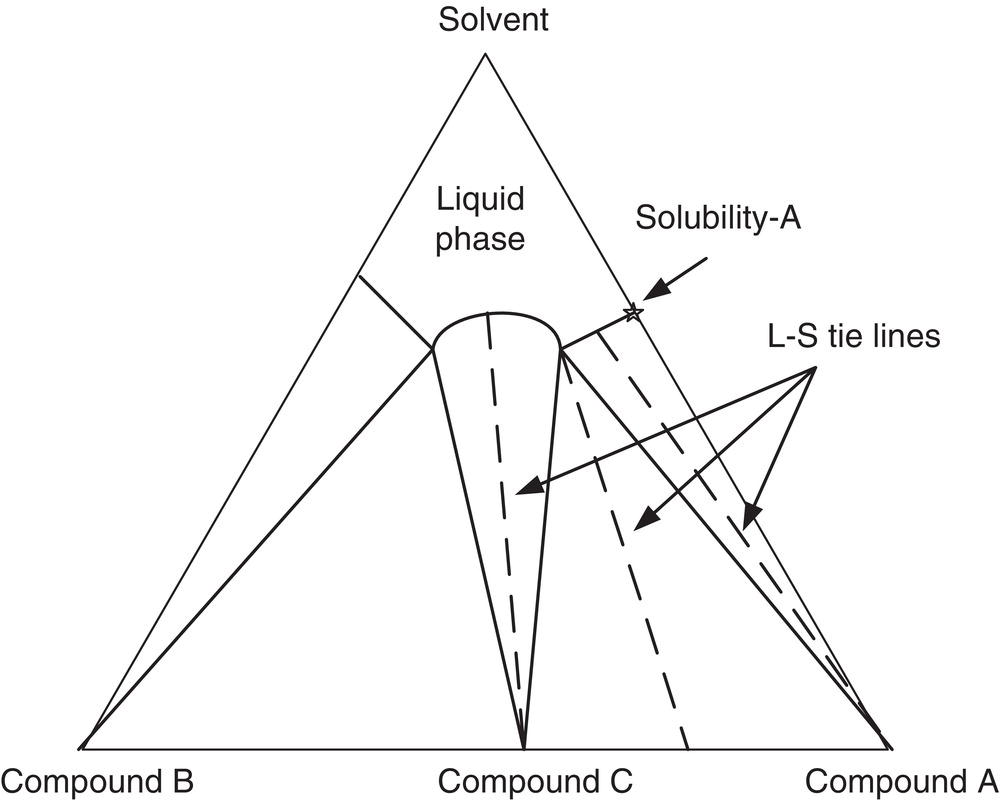
Figure 2.24 Phase diagram for the case of solid compound.
Figure 2.25 shows a generic solid–liquid phase diagram in which compound A and compound B forms a solid solution in the presence of solvent. As shown in Figure 2.25, the equilibrium liquid composition varies with equilibrium solid composition. Therefore, as long as the overall composition of the system lies within the triangular area (not along the boundary line), it is impossible to obtain pure solid compound A or B.
Salts and co‐crystals are good examples for solid compounds, i.e. compound C in Figure 2.24. Solid compound and solid solution cases are also commonly encountered in optical isomers (Sheldon 1993). Solid compound and solid solution could also exist in other structurally similar materials. Figure 2.26 shows the solubility of lovastatin and simvastatin in a solvent mixture of acetone/water. The solubilities of lovastatin and simvastatin vary and are dependent on the composition in the solid phase. This is a case of solid solution similar to the diagram as shown in Figure 2.25. As we recalled from Figure 2.6, lovastatin and simvastatin are only different by one methyl group. Since lovastatin has a lower solubility than that of simvastatin, the level of lovastatin in the solid phase will be higher in the solid phase, whereas the level of simvastatin in the liquid phase will be higher.
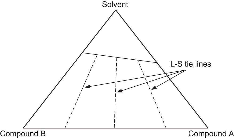
Figure 2.25 Phase diagram for the case of solid solution.
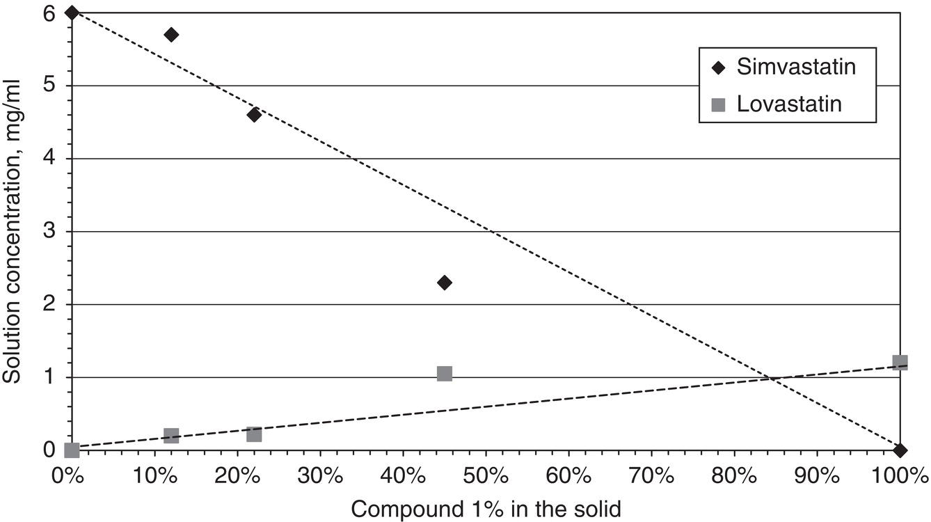
Figure 2.26 Solubilities of chemically similar APIs: lovastatin and simvastatin.
2.6.2 Measurement and Prediction
Solid compounds and solid solutions, or solid mixtures can be differentiated through X‐ray diffraction powder analysis and DSC, or other thermal analytical techniques as mentioned in Sections 2.4.2 and 2.5.2.
Solubility phase diagram could provide very useful information as well. As shown in Figures 2.24 and 2.25, solubility curve can also be used to identify the regions if desirable compounds can be isolated as pure material.
2.6.3 Significance to Crystallization
The typical example for solid compound is salt or co‐crystal formation. Purification via crystallization is a common technique. For this scenario, the solid compounds are considered to be the desired products. Chapter 10 Reactive Crystallization provides multiple examples to illustrate this approach.
Solid compounds, solid solutions and solid mixtures are also frequent phenomena for chiral or chemically similar molecules (Wang et al. 2005). From the point of purification via crystallization, the formation of solid compounds or solid solutions actually presents an obstacle, because these are undesired byproduct which is opposite to the case of salt or co‐crystal which are desired products. A complete rejection of the undesirable compound is simply impossible, either thermodynamically or kinetically. As illustrated in Figure 2.26, it is impossible to reject lovastatin as an impurity from simvastatin via crystallization. Therefore, for this scenario, adding additives or other purification techniques would be required.
For the case of optical isomers, addition of an optically active resolving agent is a typical practice to “break” the solid compounds. Depending upon the chemical structure of optical isomer, the resolving agent can be either an acid or base. The resolving agent can react with the optical isomers (reactive crystallization) and convert solid compound in its initial neutral form into solid mixture in its salt form. The resulting solid mixture can then be separated via their solubility difference (Sheldon 1993). Alternatively, if the equilibrium solubility difference between the two salts is insufficient to accomplish reasonable yield, preferential crystallization can be performed to separate the diastereomer salts kinetically. Example 7.4 presents an example on the resolution of ibuprofen‐lysinate diastereomer salts.
2.7 INCLUSION AND OCCLUSION
Inclusion or occlusion takes place when impurities or solvents are physically trapped within crystals. This situation is different from the case of solid compound. For the case of inclusion or occlusion, impurities can be occluded sporadically within crystals, whereas for the case of solid compound impurities are distributed throughout the crystal lattice. While both inclusion and occlusion stands for enclosure of solvent or impurities into the crystals, inclusion is more applicable to cases where solvents or impurities are trapped within crystal cavities during crystallization, whereas occlusion is more applicable to cases where surface liquid is trapped within crystal clusters or agglomerates during drying. In this book, inclusion and occlusion will be used interchangeably.
2.7.1 Mechanism
Inclusion can occur as a result of rapid crystal growth under high supersaturation (Mullin 2001, pp. 284–286). It is speculated that under rapid crystal growth conditions, crystal will form multiple growing layers at different heights on the crystal surface. The higher level layers may grow faster laterally along the crystal surface than the lower level layers. As a result, the outgrowing of higher level layers can seal off the surface of crystals and leave cavities within crystal lattice.
Inclusion can also occur in crystal agglomerates during crystallization. Again, it is hypothesized that under rapid crystal growth conditions, particle–particle contact in the crystallizer slurry results in agglomerates of original primary particles, and solvent can be trapped within the agglomerates.
Figure 2.27 shows a microscopic photo of a COX‐II inhibitor drug candidate. These crystals are generated in the laboratory by rapidly mixing the batch with the antisolvent. As shown in this figure, these crystals form internal cavities which trap the solvents from the crystallization. Similarly, occlusion can occur as a result of crystal agglomeration during the crystallization. Figure 2.27 also shows a scanning electronic microscopic image of the same compound generated at different solvents system. As shown in the figure, the primary particles form agglomerates, which trap the solvent within.
It may not be possible to observe the crystal cavities under the microscope. Nevertheless, based on the authors’ experience, the level of residual solvent trapped within the crystal structure can be related to the degree of nucleation over crystal growth, i.e. the higher the degree of nucleation, the higher the level of residual solvent. Example 10.3 in the book will present a case study which shows that the level of residual solvent can be related to the degree of nucleation over crystal growth.
During the process of drying (of wet cake), occlusion could occur. The presence of occlusion is primarily inferred from residual solvent profile during drying, instead of direct microscopic visualization of occlusion of crystals after drying. Hypothetically, the wet cake can be viewed as a matrix of crystal solids. Both internal pores and external surface of crystal solids can be covered with a thin layer of solvent. During drying, the external solvent will evaporate and the dissolved solute in the external solvent on the surface can crystallize. If the amount of crystallized material is sufficiently high, it could seal off the external surface of crystal solids. The solvent in the internal space is thus trapped. No further removal of solvent is possible with extended drying. This can also happen if drying from mixed solvent where the antisolvent evaporates before the solvent. It is common to observe agglomerates of dry solid and the residual solvent in the cake remain steady despite extended drying. To minimize the degree of solvent occlusion, it is helpful to keep the drying temperature below certain values so that the amount of dissolved solid in the solvent on the crystal surface is limited. Furthermore, the dryer pressure needs to be maintained sufficiently below the vapor pressure of the solvent at the drying temperature. This can ensure effective evaporation of solvent on the surface of wet cake.
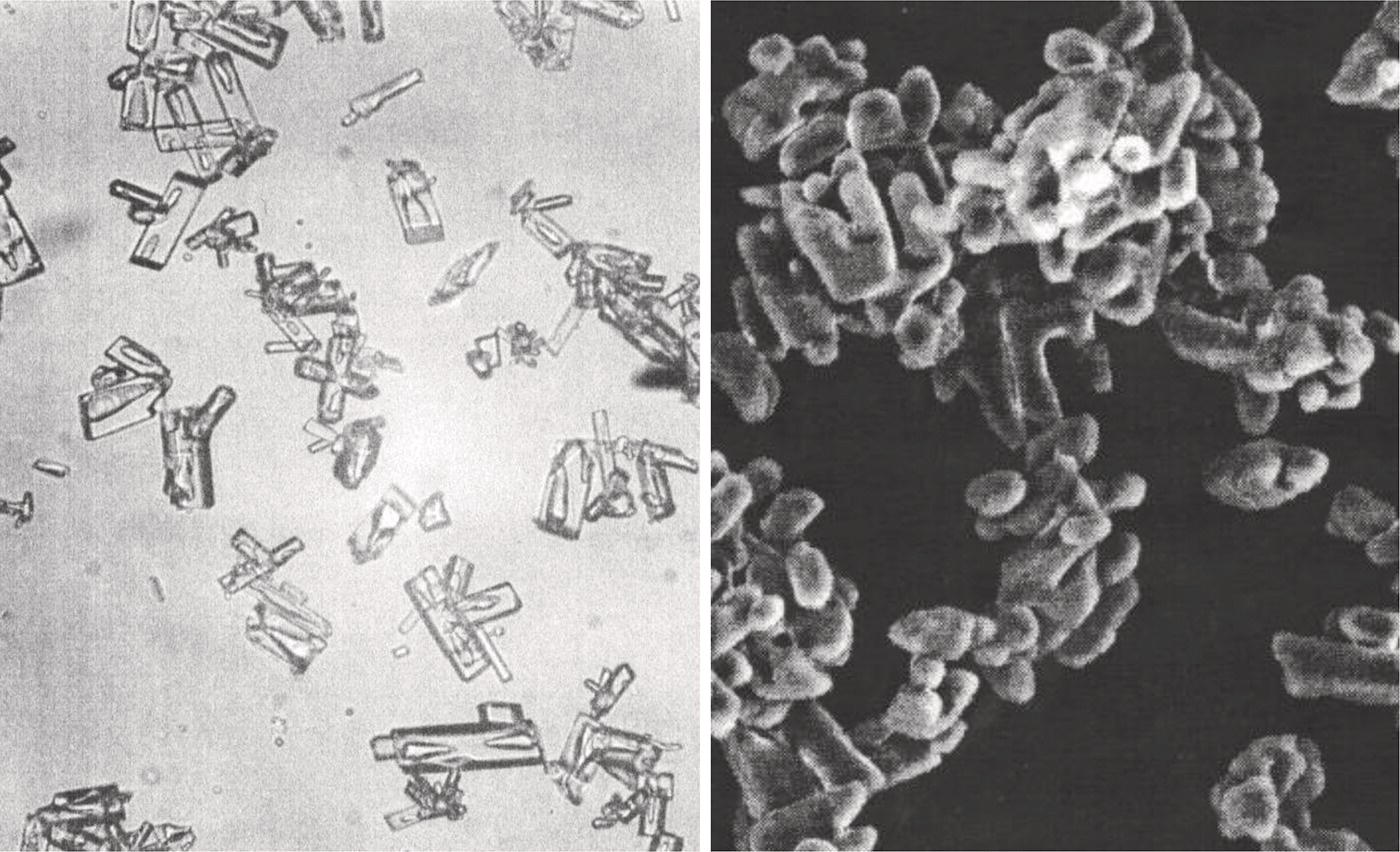
Figure 2.27 Crystal cavity and crystal aggregates.
2.7.2 Measurement
Analytically, HPLC or GC analyses are two commonly used methods in determining levels of impurities and residual solvent in the cake. Thermal gravimetric analysis is another very powerful tool. It will detect not only the level of residual solvent, but also the temperature that the solvent evaporates. If the cake weight loss due to solvent evaporation occurs at the melting point of the solid, it is a clear indication that solvent is trapped within the cake.
Measurement of impurities in the mother liquor can be conducted by HPLC. Based on the overall material balance in the dry cake and mother liquor, it provides valuable information of trends and distribution of impurities in the cake and mother liquor to differentiate various possible mechanisms during the crystallization.
As mentioned earlier, microscopic examination can be used. However, its usage is largely for illustration purpose.
2.7.3 Significance to Crystallization and Downstream Operations
From the purification point of view, occlusion presents a serious obstacle in rejecting the impurities and residual solvent. Since solvent and temperature can affect drastically the crystallization behaviors, these variables can play critical roles. Therefore, systematic screening of solvent and identification of proper crystallization conditions for optimum rejection of impurities would be desirable.
For particular solvent systems with a window of operating temperature, proper selection on the method of supersaturation generation, for example cooling and antisolvent addition, and mode of crystallization, for example batch vs. semicontinuous, can also affect overall crystal growth rate. In many instances that solvent or impurity rejection becomes critical, adequate mixing to avoid local high supersaturation can be critical. Examples 9.2 illustrate the case of rejection of impurities and residual solvent. This example will illustrate how various means are applied to overcome these complications.
2.8 ADSORPTION, HYGROSCOPICITY, AND DELIQUESCE
Impurities or solvent can be bound to crystals via a totally different mechanism. The surface of crystal can adsorb impurities or solvents from the surrounding liquid or gas phases. Consequently, impurities or solvent can distribute between the solid and liquid/gas phases. Depending upon the nature of interaction, various adsorption mechanisms have been proposed in the literature (Ruthven 1984).
2.8.1 Phase Diagram
For adsorption of impurities, the surrounding phase of interest is typically liquid phase. The adsorption isotherm can be built by determining impurity levels in the solution before and after adding the solid (as adsorbent). Based upon the change of impurity levels in the solution, the adsorption isotherm can then be determined. Figure 2.28 shows a Langmuir‐type adsorption isotherm of R‐ibuprofen S‐lysinate on S‐ibuprofen S‐lysinate crystals in an ethanol/water solvent mixture. As shown in Figure 2.28, a trace amount of impurities can be adsorbed onto the crystal surface even when the impurity concentration in the solution is well below its solubility limit.
For adsorption of solvent, the surrounding phase of interest is typically vapor phase. Hygroscopicity is a special case of adsorption in which water is preferentially adsorbed onto the crystal surface. Materials that exhibit this behavior are called hygroscopic materials. Deliquesce is a phenomenon when a hygroscopic material liquefies after adsorbing a certain amount of water onto the crystal surface. Hygroscopicity and deliquesce are commonly encountered in pharmaceuticals.
Figure 2.29 shows a typical vapor–solid adsorption isotherm of a hygroscopic material. As shown in Figure 2.29, when water concentrations in the vapor and solid phases are located below the isotherm curve, the water in the vapor phase is supersaturated with respect to the water level in the solid phase. Therefore, water in the vapor phase will be adsorbed onto the crystal surface. When water concentrations in the vapor and solid phases are located above the isotherm curve, the vapor phase is undersaturated with respect to the water level in the solid phase. Therefore, water in the solid phase will evaporate into the vapor phase. As a final point, the water vapor pressure, which is in equilibrium with water adsorbed on a hygroscopic material, should always be less than the water vapor pressure which is in equilibrium with liquid water.
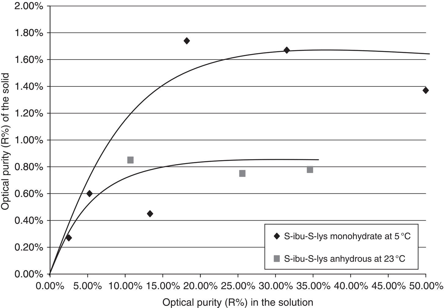
Figure 2.28 Adsorption of R‐ibu‐S‐Lys on S‐Ibu‐S‐lys.

Figure 2.29 Vapor–solid adsorption isotherm.
2.8.2 Measurement
As mentioned in Section 2.7.2, analytically HPLC and GC are two commonly used methods in determining levels of impurities and residual solvent in the cake. Similarly, thermal gravimetric analysis is another very powerful tool. It will detect not only the level of residual solvent, but also the temperature that solvent evaporates. If the cake weight loss due to solvent evaporation occurs below the melting point of the solid and near or below the boiling point of the solvent, it is a clear indication that solvent is absorbed on the surface of crystals.
The adsorption isotherm can then be constructed by determining the equilibrium solvent concentration in the vapor and solid phases over a range of solvent composition.
2.8.3 Significance to Crystallization and Downstream Operations
The efficiency of rejecting impurity via crystallization is reduced if impurities are preferentially absorbed on the crystal surface. For resolution of chiral compounds or crystallization of pure bulk pharmaceuticals, trace levels of adsorbed impurities could be detrimental if not properly treated. Fortunately, surface impurities can generally be removed with proper cake cash. Therefore, an effective wash to remove the adsorbed impurities is highly desirable.
Adsorbed solvent in general will not impose difficulty in processing since it can be removed during drying. Complications can arise if solvent in the wet cake is occluded within crystals during drying as mentioned in previous section. If a mixture of solvent is used in the crystallization, the interaction of solvent mixture on the crystal surface is affected by their affinity to crystals and can be quite complicated.
For example, in the drying of a hygroscopic drug compound, the residual solvent profile depends strongly on the relative humidity level in the vapor phase. Figure 2.30 shows the profile of residual ethanol level in the cake during drying. As shown in Figure 2.30, if the relative humidity of vapor phase is between 7 and 50%, the residual ethanol can be effectively removed from the wet cake. However, if the relative humidity of vapor phase is below 1%, the residual ethanol in the wet cake will reach a plateau and cannot be removed. If the relative humidity is above 70%, the wet cake liquefies (deliquescence) and loses its crystallinity. This example illustrates the potentially intricate interaction of solid and (adsorbed) solvents. This example also points out the potential benefit of selective drying of one solvent by controlling the vapor phase composition of other solvent.
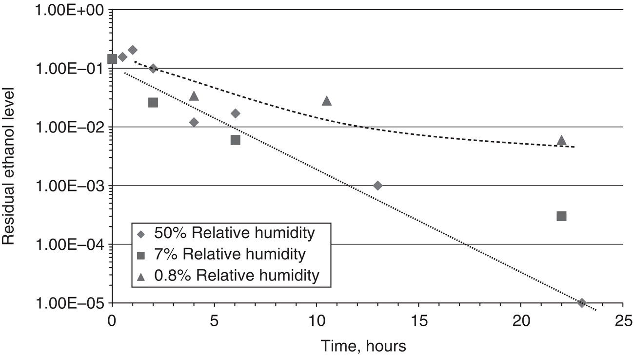
Figure 2.30 Residual ethanol level in the wet cake during drying.
Hygroscopic material requires special attention in processing and handling. In order to remove the water and keep the cake dry, it is essential to maintain a dry environment under all circumstances during drying, packaging, and storage. Otherwise, the cake would pick up moisture from the vapor phase. A wet cake could fail the product specifications or have inferior long‐term chemical stability. For certain materials, the cake may deliquesce once exposed to the wet environment and go through irreversible change of solid state to amorphous material.
The readers may recall that the above scenario is opposite to the case of hydrate as mentioned in Section 2.5.3. For the case of hydrate, it is desirable to maintain a certain level of relative humidity during drying, package, and storage. If humidity level is below a certain level, the hydrate may lose its water and dehydrate.
A detailed discussion with case study of downstream operations is presented in Chapters 11 and 12.
2.9 CRYSTAL MORPHOLOGY
One of the many unique features of crystals is crystal habit. Crystals can have different shapes and faces that make them unique and distinct from liquid or gaseous materials. In view of the focus of this book, crystal morphology as referred simply means the approximate shape of crystals. Our purpose is to qualitatively describe the aspect ratios of crystals in three‐dimensional spaces with relevance to crystallization process. Therefore, we refer reads to (Mullin 2001, chapter 1) for a more thorough and comprehensive classifications of crystal morphology.
Crystal morphology only refers to the appearance of the crystals, and does not reflect the internal crystals as described in Section 2.4 of crystal form. Crystals of different morphology can have the same or different crystal forms.
2.9.1 General Observations
Roughly speaking, over the variety of pharmaceutical compounds, it is common to observe three types of crystals as shown in Figure 2.31.
In this book, the first type crystal is called “needle‐like” crystal because it only has one key dimensional length. The second type crystal is called “plate‐like” crystals because it has two key dimensional lengths. The third type crystal is called “rod‐like” or “cube‐like” because it has three key dimensional lengths. Clearly, this is only a qualitative description of the habit of crystals.
From the shape of crystal, it is possible to infer the surface area and relative growth rates of different crystal surfaces. For needle‐like crystal, the surface for crystal growth is primarily at two ends of needle crystals. The surface along the length of needle would have a much slower growth rate. For plate‐like crystals, the surface for crystal growth is at edges of plate crystal. The surface of the plate would have a much slower growth rate. For rod‐like or cube‐like crystals, all crystal surfaces can grow at the comparable rates.

Figure 2.31 Needle‐like, plate‐like, and cube‐like crystals.
Crystal habit gives engineers very quick and useful information on the performance of crystallization process. We will address how to utilize this information in the following sections.
2.9.2 Measurement and Prediction
In practice, optical and scanning electronic microscopes are two common methods to view the shape of crystals. Measurement can be performed offline by taking samples from the crystallizer. Therefore, care should be taken to avoid complications associated with sampling. Apparatus for in situ viewing of slurry without sampling is also available, such as EasyView or Blaze Metric. The standard resolution of such device is generally a few microns, which is comparable or inferior to an offline microscope.
From the theoretical point of view, it is now possible to predict the morphology of crystals. A number of successful industrial cases have been reported (Myerson 1999). In general, it would require X‐ray diffraction data from crystals, which are generated via crystallization experiments. The advancement in theory lead to a much better understanding of internal and external orientation of molecules within crystal lattice. Commercial software, such as material studio, is also capable of calculating the theoretical crystal shape based upon the crystal structure and calculated surface energy. If the relative growth rates (and dissolution rates) information of different crystal surface is available, it is also feasible to calculate the attainable crystal morphology domain (Lovette et al. 2011; Singh et al. 2013). As expected, modifying the relative crystal growth rates of different crystal surfaces can alter the crystal morphology. Cases have been reported which can customize the shape of crystals by adjusting the relative growth rates of different surfaces via additive or solvents (Winn and Doherty 2002).
2.9.3 Significance to Crystallization and Downstream Operations
Understanding shape of crystal because of difference of crystal growth rates on different surfaces is helpful for the development of crystallization processes. Roughly speaking, needle‐like crystal has much less surface area for growth. Consequently, more seed is required to provide enough surface area for crystal growth. On the other hand, rod‐like or cube‐like crystals have much more surface area for growth. So, less seed is required. Furthermore, it is common to observe that the fastest growing surface outgrows itself and disappears. Therefore, the apparent release of supersaturation by crystal growth is significantly reduced after certain point of crystallization. If it occurs during the middle of crystallization, the supersaturation will build up and a short burst of nucleation could occur. This will lead to a much wider PSD that is generally undesirable.
Needle‐like crystals create additional process complications, and so are plate‐like crystals. For example, needle‐like or plate‐like crystals generally have a higher filtration resistance, poor filtration and washing, breakage of particles during handling, and poor solid flow characteristics for formulation, than cube‐like crystals. Therefore, it is highly desirable to grow thicker crystals. To grow “thick” crystals, experimentally, we should try to find the best solvent which favors the formation of “thick” crystals. In the meanwhile, solvates and hydrates may form under different solvent environment. Chemical forms, such as salt, free base, and free acid, can also be evaluated. Also, control of release of supersaturation and selection of crystallization conditions to enhance crystal growth over nucleation, which are addressed in the later chapters, would be very helpful.
Additionally, it is proven that a few heat/cool cycles coupled with wet milling at the end of each cool cycle can be effective in modifying the crystal morphology. Figure 2.32 highlights a hypothetic two heat‐cool cycles with particle breakage on crystal aspect ratio (L1/L2) where L1 and L2 are the two characteristic length of the crystal. At the end of initial cooling, the aspect ratio is 10/1 (point G0). Following the path of particle breakage (point B1), heat/dissolution (point D1) and cool/growth (G1), the aspect ratio of the crystal can increase to 7/2 after the first cycle. At the end of second cycle, the aspect ratio can improve to 6/3. Based upon authors’ experience, three to five heat/cool cycles with wet milling are sufficient to evaluate the effectiveness of this approach. Besides the inherent crystal growth and dissolution characteristics of different crystal surfaces, the type of wet mill and the cooling profiles are two key processing factors in affecting the effectiveness of this approach. As shown in Example 7.3, the crystals in the slurry were sonicated repeatedly through multiple crystallization cycles. Sonication breaks one crystal into two or more pieces along its longest dimension. This effectively reduces the length of crystal or the apparent growth rate in this dimension. In the meanwhile, the thinner dimensions of the crystal continue to growth without being affected by sonication. As a result, the crystals grow thicker and shorter as time proceeds.
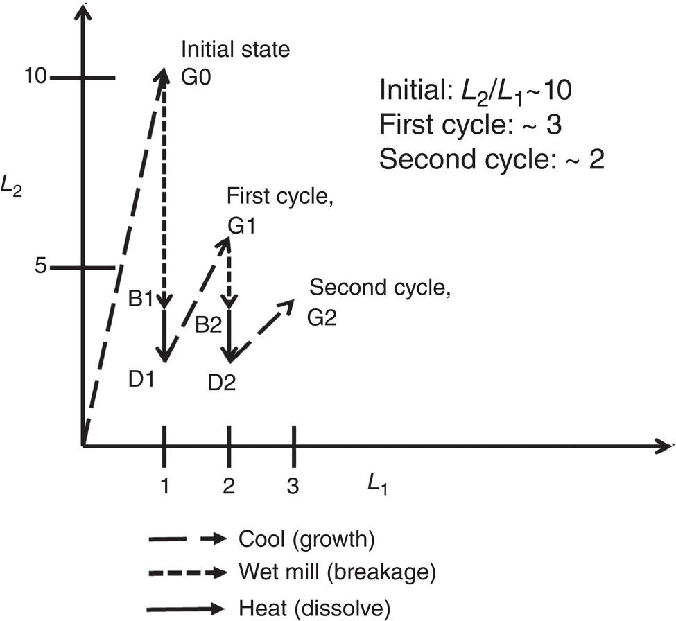
Figure 2.32 Heat/cool/wet mill cycles for improvement of crystal aspect ratio.
In practice, this approach has been applied successfully over the years in pharmaceutical industry. One key advantage of this approach is that it does not alter solvents or add additives during the crystallization, versus the other approaches such as spherical crystallization (Sheikh et al. 2008; Chen et al. 2019) or coprocessing of drug and excipients (Schenck et al. 2020). Therefore, this approach will not affect the impurity rejection or crystal form. As a matter of fact, this approach can improve the rejection of impurities by minimizing occlusion/including during the crystallization. It further enhances the robustness of the crystallization process in generating the most stable crystal form since crystallization/nucleation kinetics is accelerated during the wet milling/sonication period (Lo et al. 2012). It suffices to say that at present, there is a sufficient amount of know‐hows of this approach for effective and practical implementation.
2.10 PARTICAL SIZE DISTRIBUTION AND SURFACE AREA
PSD is another unique feature of crystals. Crystals have different shapes, and crystals have different sizes. PSD function is a very effective way to describe the distribution of particle size of crystals over a wide range of size. Although crystals have three‐dimensional length, one‐dimensional PSD function is frequently used in practice. Extending the one‐dimensional PSD function to two‐dimensional or three‐dimensional PSD functions may be closer to reality. But these functions certainly are more complex and their advantages over one‐dimensional PSD function are not always apparent.
Mathematically, the one‐dimensional PSD function can be expressed as n(L) where n is the population density function and L is the characteristic crystal length. For cube‐like (or spherical) crystal, the characteristic length is approximately the diameter of crystal. For other shape of crystals, there are various definitions for the characteristic length. Most commonly, the characteristic length of the particle with irregular shape is defined as the equivalent diameter of a sphere which has the same behaviors under the measurement conditions, for example sieving, laser scattering, sedimentation, etc. (Mullin 2001, chapter 2).
2.10.1 Particle Distribution Definition
By definition of n(L) above, N(L1, L2), which represents the total number of particle within size range between L1 and L2, can be expressed as

While the total concentration of particles, NT is given as

All other formulae can be derived based on the above definition. For example, A which is the surface area per unit mass of crystal, can be expressed as
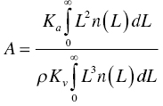
where Ka is the surface area shape factor, Kv is volume shape factor, and ρ is the density of the crystal.
For spherical crystals, L is the diameter of the sphere, Ka equals to π, and Kv equals to π/6.
For discrete calculation, the n(L) can be replaced by q(xi), and N(Li) can be replaced by Q(xi) as below:
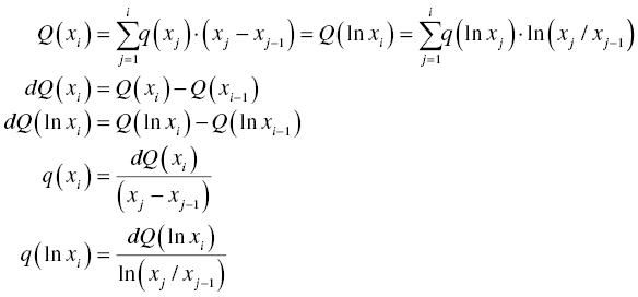
It should be pointed out that Q(xi) and Q(ln(xi)), or q(xi) and q(ln(xi)), are mathematically equivalent. The former expression is defined over the linear scale of length, whereas the latter expression is defined over the natural log scale of length.
Care should also be taken to differentiate the difference among Q, dQ, and q as shown in Figure 2.33. Very often, the analytical instrument reports only the total number of particles from xi − 1 to xi over a range of particle size xi , i = 1, … n. It is a common mistake to take the data and treat them as function q(xi) for the subsequent calculation. In reality, the reported value is actually dQ(xi) since it represents the total number of particle from xi − 1 to xi.

Figure 2.33 Particle size distribution functions, Q(x), dQ(x), and q(x).
Another common mistake in calculating the PSD data is mixing the linear scale and natural log scale. To calculate q(ln (xi)), the correct formula is dQ(ln xi)/(ln(xi/xi − 1)), instead of dQ(ln xi)/(xi − xi − 1)
2.10.2 Measurement
Various methods have been used to measure the PSD. These methods include sieving, laser scattering, sedimentation, image analysis, etc. Among these methods, laser scattering approach, such as HELOS or Microtrac (forward scattering device) or FBRM (back scattering device) is widely used in industry.
Instrument for online measurement of either dry or wet system is also available. Due to the diversity of measurement techniques and definition of characteristic length, different types of instrument most likely will give different PSD for nonspherical particles. Therefore, it should be understood that there is no absolute standard for PSD measurement.
Another perplexity of PSD measurement is caused by particle agglomerates. A single large agglomerate may contain multiple small crystals. But this single large agglomerate will be counted as one large particle if it is not dispersed during the measurement. In consideration of this, it is always desirable to have microscopic examination and surface area measurement, in conjunction with PSD measurement.
Surface area of crystal is typically measured through BET technique. The measurement of surface area is much more consistent among various vendors.
2.10.3 Significance to Crystallization and Downstream Operations
PSD can be considered to be the second critical physical attribute for pharmaceuticals, next to crystal form. Control of PSD is critical for various aspects of drug product and its development. Unimodal distribution of particle size is generally preferred over bimodal, or multimodal distribution. For drugs with low water solubility, generally it will require fine particles with narrow PSD. Other than milling, special techniques, such as impinging jet crystallization as shown in Example 9.6, are sometimes employed to meet such requests. PSD, especially in the submicron range, plays an important role in the dissolution or bioavailability for water‐insoluble compounds. PSD can also affect other critical aspects of drug product such as blend content uniformity. For drug product of low drug loading, for example <10 wt%, smaller particle size is preferred. For downstream operations, fines may breakthrough the filter, slow down the filtration rate, and/or reduce the overall yield. Therefore, proper control of crystal size by crystallization (and/or milling) is essential.
Information of PSD during the course of crystallization can provide valuable insight into the nucleation and crystal growth behaviors of the system. An increase in total particle count and decrease in particle size could represent nucleation which can lead to impurities trapping, formation of undesired crystal form, or contamination of undesired optical isomer for chiral resolution. An increase in particle size with similar particle count could mean crystal growth, which will minimize impurity occlusion and ensure desired crystal forms, etc. Example 7.2 gives an example on the use of online monitoring PSD for the development of crystallization process.