Chapter 9
Optimizing DSP Software – Benchmarking and Profiling DSP Systems
Chapter Outline
Test harness inputs, outputs, and correctness checking
Protecting against aggressive build tools
Allowing flexibility for code placement
Modeling of true system behaviors
Execution in a multicore/multidevice environment
Methods for measuring performance
Performance counter-based measurement
Introduction
A key part of optimizing DSP software is being able to properly profile and benchmark the DSP kernel and the DSP system. With a solid benchmark and profiling of the DSP kernel, both best-case and in-system performance can be assessed. Proper profiling and benchmarking can often be an art form. It is often the case that an algorithm is tested in nearly ideal conditions, and that performance is then used within a performance budget. Truly understanding the performance of an algorithm requires being able to model system effects along with understanding an algorithm’s best-case performance. System effects can include changes such as a running operating system, executing out of memories with different latencies, cache overhead, and managing coherency with memory. All of these effects require a carefully crafted benchmark, which can model these behaviors in a standalone fashion. If modeled correctly, the standalone benchmark can very closely replicate a DSP kernel’s execution, as it would behave in a running system. This chapter discusses how to perform this kind of benchmark.
The key ingredients to a proper benchmark include being able to build the DSP kernel as a single isolated module. Modularity helps to isolate a kernel for testing and measurement. A DSP kernel should always be separated from its test harness and from the runtime libraries used by a test harness. Modularity also ensures that when it is implemented in a system along with other kernels, it is still measurable and comparable to any standalone benchmarks. Also of key importance is to create a flexible test harness. This should be code that is able to exercise the kernel, possibly multiple times, provide a means of measuring the performance of the kernel, provide input test configuration, input test vectors, output test vectors, and often act as a means to self check an algorithm for correctness. Other test harness considerations should include being able to move code and data content to and from memory regions with differing latencies and cache policies, and to be able to adjust memory sizes and allocations such that the algorithm can more closely replicate how it would behave in a fully operational system.
Writing a test harness
The best method for getting optimized code is to break the work into modules with distinct and measureable inputs and outputs. In this way a DSP functional block or kernel can be worked on in isolation. This removes system impacts such as operating systems, interrupts, and other system-level interference from impacting performance measurements. By isolating a DSP kernel, its performance can also be isolated, measured, and re-measured to show improvements or degradation in the kernel’s performance. Getting the best possible performance in a DSP kernel, in isolation, almost always results in getting the best performance from the algorithm once it is integrated back into the running system.
In order to properly test and measure the performance of a DSP kernel, it is typically ‘wrapped’ in a test harness. A test harness is simply a bit of standard C code (typically) which is used to test the DSP kernel. Writing a test harness is not difficult, but it requires some careful planning. A consistent methodology should also be used so that the harness itself is re-usable, extendable, and consistent with other DSP kernel test harnesses. Other things to consider in writing a test harness include profiling capability of the hardware or simulator, ease of substitution of new versions of a DSP kernel, the ability to automate the testing and profiling process, and the profiling or optimization goals. A test harness for a DSP kernel should be able to:
• Handle multiple input and output vectors in a manner that does not impact the kernel’s functionality or performance
• Isolate a DSP kernel for testing and profiling purposes
• Verify results with a ‘golden’ model or other reference vectors
Test harness inputs, outputs, and correctness checking
Test harnesses all require a method for input of test vectors outside of a real system. This is normally achieved either by reading the vectors from an external text or binary file, or by placing the vector data within the test harness’s memory. In modern DSP systems, one of the more critical aspects of optimization is code placement in various memories. Latency and cache policy can vary significantly from external to internal memories and from architecture to architecture. So placement of input control structures and data, output data, and other results is critical in creating a test harness, which gives realistic performance numbers. The test case itself should be allowed some flexibility in its memory placement, so that performance tuning can be performed based on code and data location. The inclusion of data vectors can be carried out via several methods. Common approaches include:
• Placing the test vector data inline in a header or source file
#include “my_input_vector.dat”
#include “my_control_parameters.dat”
• Using a #include “my_vector.dat” inside a variable definition or for the variable definition
UINT32 my_IQ_buffer[] = {#include “my_vector.dat”};
• Reading the data from an external file
FILE input_file;
Char my_input_filename[] = “./../../vectors/my_input_vector”;
if ((input_file = fopen(my_input_filename, “rb”) == NULL)
{
return (FILE_OPEN_ERROR);
}
//Read the file
.
.
.
//Close the file
fclose(input_file);
• Pulling the data using a development tool script
#Load the Input Buffer with the Input Test Vector and Go
## Input Test Vector Naming Convention --> IF2_Tx_<sbfn>_<user_id>_<rvindex>.lod
set TVIn _$RVIndx.lod
set TVIn _$UserId$TVIn
set TVIn _$SubFrN$TVIn
set TVIn IF2_Tx$TVIn
set TVIn /$TVIn
set TVIn ..//..//vector/in/TC$TC$TVIn
set dummy_addr [evaluate #x dummy_sequence]
set in_addr [evaluate #x IF2a_Tx_Data]
puts “input_sequence =”
puts $in_addr
restore -b $TVIn m:$in_addr
restore -b $TVIn m:$dummy_addr
go 10000
These approaches each have some benefits and drawbacks of course. Placing vectors inline with the test bench can lead to difficulty changing the test vectors and can also lead to very large source files which may take longer for a compiler to parse. Also if multiple buffers of a large size need to be placed sequentially or randomly, inline data sizes can grow significantly. Using a #include statement allows for an external text file to be used, which tends to be easier to change for updates to test vectors, and also makes for cleaner, more readable code. However, it has the same drawbacks for compile time and space usage. In all of these cases, changes such as swapping to a different set of test vectors would generally require a rebuild, unless all test cases could fit into memory, but again for general debugging, this has drawbacks as well. This approach tends to limit the number of test cases that can be run, so keep this in mind when developing a test bench. Reading data from an external file is also a typical approach and this tends to be the most flexible one for updating test vectors, as it typically requires no rebuild of the test bench itself. Most Silicon vendors provide at least a basic <stdio> library which includes functions such as fopen, fread, fwrite, fseek, fclose, and printf. A drawback of this approach is that it adds runtime library code to the test harness and it may have an impact on the test execution’s performance if care is not taken to exclude any cache or IO operations which may take time from the test harness’s execution. Runtime effects can be mitigated by judicious use of cache control operations such as synchronizing or flushing around the runtime library calls.
In both cases care should be taken in the scope of the input data relative to the function being tested. This is particularly important when using global optimizations. It is often the case where compilers will constant propagate or even dead strip algorithmic code if it can find an optimal solution. This can lead to misleading results and incorrect behavior modeled from a single test vector rather than an entire system. (Example of a flag being const propagated, or an output becoming the answer). For example in the following code sequence:
my_config = TEST_FOR_120_FRAMES;
if(my_config == TEST_FOR_60_FRAMES)
In this example code the if-else ladders which would call RLSIP_Frame60() and RLSIP_Frame180() would be optimized away, and If this is the only place these functions are called the functions themselves could be dead stripped. Additionally, no comparisons for my_config would occur. This could change the code layout which can impact instruction cache performance and removes some comparison functions which changes how the code is generated by the compiler.
Isolating a DSP kernel
Isolating a DSP kernel is a straightforward process. The best approach here is always to keep any code that will be running on the target system in some form or another in its own source files and header files. This prevents a compiler from doing things that would not occur in the real system, such as moving functions inline with the test harness, constant propagation, and in some cases, algorithms or control code being stripped and replaced with results. This can all occur if the test kernel is within the same scope of the test harness and test input vectors. Also, if global optimizations are available, then these should either not be used, or should be used with caution. If they are helpful, then using a pragma to disable automatic inlining might be a good idea, but this may not prevent constant propagation, which would essentially remove code dependent on values perceived as constants by the compiler.
Protecting against aggressive build tools
Some build tools will optimize away significant portions of an algorithm or control code. This often occurs when using global optimizations or if the test vectors, input control structures, or even the output data is within the scope of the compiler to optimize away. For example, if testing for a case where control code has four options and only one of the four are used in the test vectors, an aggressive compiler may throw away the control paths for the other three options. Additionally, if the output data appears not to be used, some compilers can decide to skip the algorithm entirely. Care should be taken in specifying the scope and global compiler options. It is also often a good idea to inspect assembly listings to verify that code is in place for parts of the DSP kernel being tested and also for parts that may not be exercised by the current set of test vectors. If the results look too good to be true, in general they are.
Allowing flexibility for code placement
In modern DSP systems, object placement is often critical to the overall system’s performance. Multiple levels of internal and external memories are available, and it is often necessary to be able to move test harness code, test vectors, output vectors, kernel code and kernel data to lower or higher latency memories. This is typically done at link time, and less often in a dynamic environment. Keep in mind questions such as:
• Where would input vectors be in your software design?
• Where do output vectors go in your design?
• Where is the DSP kernel going to be?
• What is the size of these objects and will they all fit into a low latency memory?
• Do you need to model the benchmark as it would be in your system or can some assumptions be made?
• Will there be multicore effects such as reduced bandwidth to some memories?
• What will the cache loading be when your algorithm starts?
Modeling of true system behaviors
Cache effects
Today with DSP kernels, it’s really all about the caches. Level 1 caches tend to be zero wait state, and ideally a DSP kernel executes from cache for both instruction and data accesses. To run a fair test, a developer needs to know what the status of data should be in caches. Does the system support hardware coherency or does it require software coherency support? Is it a mix of these two? Is it data coming from a DMA copy? Is it located in an external high-speed interface? In these cases the data would not be in the caches at all when the kernel first starts. Is it appropriate to prefetch the data or instructions in the kernel or in the test harness? Does the test harness also occupy space in the caches prior to running the kernel? Is this a valid state for the hardware or should test harness code and data not being used by the kernel be flushed? Does a run with the cache not initiated, or cold, give a valid representation of the kernel benchmark or does a warmed cache run make more sense? Data and instruction alignment is also often used as a cache optimization. Other considerations should include the cache behavior for fetching, synchronization, flushing, and invalidation operations.
Memory latency effects
Memory latency has a large impact on a DSP kernel’s performance. A developer must understand the latencies to various memories, but even more, the rules of thumb of any memory controllers with regard to access alignments and page switching.
System effects
RTOS overhead
An RTOS adds overhead. Even the thinnest, barest RTOS will be written to the lowest needed API functionality of a system. Additionally, it allows a DSP kernel to run in a much more realistic environment and it often makes porting a DSP kernel into the overall system less time consuming, as much of the work in integrating the algorithm with the RTOS is already completed. Considerations here include the RTOS’s usage of system resources such as low latency memory and caches, and also any differences in the system configuration enforced by the RTOS. Other considerations include the overhead of the RTOS, as well as interrupts, which in a standalone test case are seldom enabled, but are in general always enabled under an RTOS, unless explicitly disabled.
Execution in a multicore/multidevice environment
It is quite rare to test a DSP kernel in a multicore environment. This is because this kind of testing is difficult to do, and unless a full system is ready, it does not give an indication of the true multicore system’s effects on algorithm performance. These effects include the potential for longer memory stalls, lack of availability of peripherals and other system resources, interrupts which would not occur in a single core system, changes to system timing, and even to order of execution. Also, with multicore systems there is often a need to synchronize messaging and data exchange between cores.
Methods for measuring performance
There are many methods of measuring performance on a DSP system. These include time-based measurements using a real-time clock, hardware timer or RTOS tick counter, performance counters which run at the core clock rate or an integer division of the core clock rate, or at its most basic, using IO triggers and a logic analyzer or oscilloscope. This latter method is often unnecessary for anything but a sealed or very simple DSP system.
Time-based measurement
Time-based measurements are the most frequently used methods of measurement in most modern DSP systems. Most RTOSs provide a timer service of some kind that can be co-opted for performance measurements. It is also often an RTOS event, which is used as a trigger point to enable and disable measurements. For example, an RTOS context switch to and from a task is often a simple way to take measurements and many RTOSs provide hooks in the context switch code of their kernels to easily create these measurement points.
Hardware timers
If a service is unavailable, or not precise enough, for use in benchmarking, then a hardware timer can also be used. This approach has the big drawback of using a hardware resource (the timer) for what may be a non-essential task. When using hardware timers it’s a good idea to verify the input clock frequency, pre-scale settings, and general operation of the hardware timer. It sometimes makes sense to output the timing to a scope to verify and sanity check that the settings being used correspond to some real-world fixed timing and that no mistakes or omissions have occurred in the documentation for the device being used.
Performance counter-based measurement
Most DSP cores today offer 32- or even 64-bit performance counters, and often multiple counters are provided. These are often capable of measuring precise numbers of clock cycles since they run at the same clock rate as the core itself. Some hardware will give additional inputs to the counters to measure other system activities as well. These include cache misses, memory subsystem accesses, stall occurrences, speculation success rates, and other useful details on what is happening within the DSP kernel being tested. Some of these hardware blocks even allow for advanced triggering to enable and disable the profiling at specific locations in the code based on prior execution paths, data patterns, counted events or cycles, or other events.
Profiler-based measurement
Many DSP devices have built-in profiling hardware. This hardware is useful for point to point profiling, often showing a function or loop level of resolution. For more in depth resolution there are many simulators, which can show performance at an instruction-by-instruction resolution. This level of resolution is often very useful in fine tuning and optimizing a DSP kernel. It is often the case that these profiling capabilities are exposed by a development tool and are often one of the more complex aspects of the development tool. Using these features can sometimes be difficult. In these cases seeking assistance from the tool vendor is usually a good option to pursue.
Measuring the measurement
When taking very accurate measurements of a DSP kernel, or when running test vectors that do not create more than several hundred cycles, it is important to measure the latency of your measurement technique. This is often performed as a read of a counter and perhaps some small calculations for offsets of the count values. Latency to hardware counter registers and other memory mapped registers in an embedded system can vary quite a bit. Typically latency to these registers can be anywhere from 25 to 80 cycles! This means that if your DSP kernel executes in 400 cycles, the activity of reading registers may account for 20% of the total benchmark number! A typical approach to this would be to place a few assembly ‘nop’ instructions in a test function, and to measure the number of cycles it takes to benchmark that function. It will include the nop function and also the latency of reading the counters in the final number.
Excluding non-related events
When running a DSP kernel benchmark there can often be unrelated events that might impact benchmark results. These include system interrupts, runtime library functions, and other hostio-based interactions that might be used in the benchmarking process.
Interrupts
Interrupts, if at all possible, should be disabled during a benchmark. Many profilers do not distinguish between the context of being in a DSP kernel and being in an interrupt service routine. This means any interrupts which occur mid-benchmark will usually have the cycles associated with them buried in the benchmark results. If interrupts cannot be disabled, then care must be taken to exclude the interrupt prologue, epilogue, and body from the benchmark results. Also be aware that executing an ISR will have an impact on cache behavior, especially instruction cache behavior, as it is essentially a change of flow and often one that speculation will not predict. This may also impact branch speculation by evicting some of the DSP kernel’s already present speculation entries from the hardware’s speculation lookup tables. Interrupts do change the benchmark behavior, and in almost all cases, they will degrade benchmark performance. If performance increases in the presence of interrupts, it would be advisable to carefully check what is happening, as it may be indicative of cache thrashing or a software error.
Runtime library functions used in the benchmark
Runtime library code is a valid item to measure and to use within a benchmark. Care should be taken around ‘special’ functions that may interact with the hardware debug environment or the simulator environment. Functions that perform any kind of file IO or console IO, or accelerate memory clearing for simulation, should be used with caution. Contact the tools provider to find out which of these functions might change its behavior based on real-world execution versus execution in a debug environment.
Simulated measurement
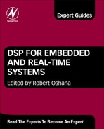
Modern simulators for DSPs have become very complex, and are now able to simulate hardware timing behavior to a very high degree of accuracy and precision. That said, many vendors offer multiple simulator models with varying degrees of hardware modeling. These can be something very basic, such as an instruction set simulator (ISS), which performs a functional modeling only. Timing information in this model is not generated, nor is it available. These are often used to check functional correctness on simulations that may run too long on a more complex model. The more commonly used simulators for profiling and optimization purposes are labeled cycle accurate simulators (CAS) or performance accurate simulators (PAS). These can model behavior from the DSP core to the DSP subsystem to the entire device. Additionally they model caches, cache controllers, memory busses, and latencies to provide a very accurate accounting of everything that executes within a DSP kernel. Often these simulators have software hooks enabling a very large amount of detailed information to be gathered during profiling. Details on cache behaviors, core stalls, memory stalls, and an instruction-by-instruction account are all made available in these simulator models. This makes them an excellent choice for profiling and optimization work on standalone kernels or code which does not require external stimuli such as hardware interrupts or external ports or busses.
Figure 9-1 shows a sample profiling output for a DSP kernel. Each line of disassembled code which executed has core stalls, data bus stalls, and program bus stalls associated with them. Developers can use this information to better understand the details of how their software interacts with the hardware.
Figure 9-1: Critical Code analysis view.
Simulator models also present a model for onboard profiling hardware as well. This is particularly useful when detailed views of the system may not be necessary, and also to do back-to-back comparisons of the simulator’s results against actual hardware. By providing a model of profiling counters in the simulator code which reports from these counters will work identically on both the simulator and on actual hardware.
Hardware measurement
Measurements on hardware are often simpler than what is available in a simulator. Often the hardware provides one or more high-speed counters and several hardware timers which can be used for profiling purposes. In some cases hardware trace can be configured to add these counters as tags to each trace message. When making measurements it is always a good idea to ask the vendor to provide any software setup code or detailed documentation on the profiling hardware. Some of the key questions about using hardware profiling counters are:
• What should the counter’s initial value be?
• Does it interrupt on overflow or underflow?
• Does the counter run at the core’s clock rate or a division of it, or from an external oscillator?
• Are there any pre-scale factors or other scaling factors that would affect the count rate?
Other considerations for hardware counters would be to check if they are accurately modeled in a simulator. This would allow use of these counters both with hardware and while hardware is inaccessible. It is often the case that some of the counters may be modeled while others are not.
Profiling results
Profiling results can be in the form of a database full of trace messages, or can be a simple reporting of a counter, scaled to some meaningful value relevant to the benchmark being run. Results will vary, and it is important to be able to identify quickly and easily where the majority of cycles are being spent in a DSP kernel. Some tools provide detailed information to identify these areas (see Figure 9-1). Also profiling results shows by inspection, core stalls, data accesses, cache misses, control code paths, and even branch speculation behaviors.
How to interpret results
Interpreting results should be done with some care. A close inspection of the assembly code is really the only method to truly ensure that the benchmark makes sense and does what was expected. The reason for this is that modern DSP compilers tend to obfuscate code, and they can strip code unexpectedly in a benchmark as being “dead” simply because the benchmark may not use a particular code path. By inspecting the code items such as how parallel the arithmetic operations are, algorithm efficiencies, and control code efficiencies can be determined. These items can be used to select areas to optimize by re-working the DSP kernel, and tend to be the valuable part of testing and benchmarking once the basic goal of functional verification is achieved.