Chapter 14
DSP Operating Systems
Chapter Outline
Processes, threads and interrupts
Virtual memory and memory protection
Preemptable vs. non-preemptable scheduling
Blocking vs. non-blocking jobs
Multicore considerations on scheduling
Offline scheduling and its possible implementation
Online scheduling (priority based scheduling)
Introduction
Digital signal processors (DSPs) were first introduced commercially in the early 1980s with the first widely sold TIs TMS322010. The first DSPs had a very limited set of external interfaces (TDM, host interface), and high level language compilers were not available at all, or were not producing very efficient code. Most of the applications were focusing solely on ‘data crunching’ and did not contain much control code or multi-threaded execution paths. This is why, in the early days, most of the DSPs were utilizing the ‘bare-metal’ model where all the resources belonged to and were managed by the application itself, only rarely using very basic, typically home-grown OS code. This situation gradually changed during the early 1990s, mostly due to the emergence of the 2G wireless technology. Wireless infrastructure projects, more complicated peripherals, and networking stacks changed the basic requirements for OS support. More recently, the introduction of multicore heterogeneous and homogeneous platforms also affected basic requirements. As a result, we see that the importance of OSes has grown over the years. Firm evidence for this is the fact that two of the leaders in the DSP market (Texas Instruments and Freescale) nowadays provide their own, proprietary OS as part of their offering and this situation is markedly different from the 1980s and 1990s. It means that those companies recognize the importance of the OS offering and invest resources in this area. This chapter should provide a good introduction for DSP engineers and also contains some in-depth discussion on multicore and scheduling.
DSP OS fundamentals
What is an OS and what is an embedded OS? Generally speaking, OS responsibilities are twofold:
• Resource management: It includes computation resources sharing and management (multitasking and synchronization), I/O resources allocation, memory allocation, etc.
• Abstraction layer: provides a way to achieve application portability from one hardware platform to another
From this point of view, there is no principal difference between an embedded OS and a desktop OS – the difference is only in the set of peripherals/resources managed and in the typical applications supported. So, what is the most typical quality of an embedded system? We would suggest that an embedded system is focused on a limited amount of applications/usages. It allows the design of a system using scarce resources.
Real-time constraints
DSP is all about real time and this is why real-time considerations are such an important factor in the design of an OS for DSP. Real-time constraints for a job mean that it has to produce results before some predefined deadline.
Real-time constraints of the job may be described using a usefulness of results function. This function is a relation between time and usefulness of the job’s result as shown in Figure 14-1.

Figure 14-1: Usefulness of results in a real-time system.
In Figure 14-1, job A has hard real time constraints because its usefulness function breaks sharply at deadline and is equal to zero (it may even be negative in some cases). The term real-time OS is somewhat confusing: real-time constraints always exist on a system, at application level, and an OS may only support the system to satisfy those constrains. So, it is important to be aware of the fact that using real-time OS does not guarantee that the system will be real time.
If we think about real-time constraints in the broader context of ‘real-time job must produce results before some deadline,’ we notice that it implies that this job must be able to get all the resources it needs. In OS terms it means that resource allocation cannot fail for real-time jobs. In many cases, it means that all the resources for real-time jobs must be allocated in advance, even before the job is ready to be executed. If we talk about jobs that are cyclical or sporadic, those resources may never be released back to the system.
Processes, threads and interrupts
Surprisingly, there is some confusion around terminology in that area. Different OSes differ in what terminology they use to describe those entities. In this chapter we will use the following definitions of OS terms.
Process
Entity that consists of complete state of a program and at least one thread of execution. Classic processes are hardly ever used in DSP RTOses. There is a tradeoff that exists between protection that OS guarantees and performance that one can achieve with such protection. For example, having user and supervisor modes would help tremendously to protect the kernel from user-level applications but at the same time might affect performance if each call to OS were to go through a system call interface. Another example is task-switch time that would grow significantly if the entire memory management unit (MMU) context had to be switched.
Thread
Schedulable entity within process. In some cases, it is beneficial to have several threads of execution within the same process. They share the same memory so it is possible to efficiently share data between them; there is no high cost of process switches (no need to switch memory context). In most DSP RTOSes, only one process will typically exist, meaning that the entire memory space is shared between all the threads. To make things more complicated most RTOSes call those threads tasks.
Task
Task is a type of thread that is scheduled by RTOS scheduler. It is different from hardware interrupt and software interrupts by having its own context where task state can be saved and restored. Typically, it has the following states:
Interrupt
Interrupts can be seen as a special type of thread that is executed in reaction to hardware events. It is scheduled by OS and is executed in the context of OS kernel.
Interrupt latency
Interrupt latency measures the maximum response time of the system for a particular interrupt. In other words, how long it takes at maximum for specific interrupt service routine to be called in response to an interrupt. This parameter is important for real-time systems because they respond adequately fast to external events. Figure 14-2 describes interrupt latency as a function of contributing factors.

Figure 14-2: Interrupt latency as a function of contributing factors.
Interrupt latency is a sum of several elements:
• Hardware latency – time from event itself to first instruction executed from interrupt vector if interrupts were not disabled. It is typically the smallest part of interrupt latency.
• Interrupt disabled time – many OSes kernels use global interrupt disable instructions in order to guard local accesses to shared variables.
• Higher or equal priority interrupt is active – if higher or equal interrupt is active, lower priority interrupt cannot run and it adds to interrupt latency for this particular priority.
• Interrupt disable for particular priority – in some cases it is important that interrupts of particular priority and lower are disabled. For example, the system may have a specific thread (which is not interrupt service routine (ISR)) that is hard real time and it is important that none of the lower priority interrupts can interfere with it. In such a case, the user would set current ISR priority to an adequate level. Some OSes will have unified priority schemes for threads and interrupts that will do this automatically (OSE) and some will allow manual configuration (SmartDSP OS).
• Interrupt overhead – several actions that OS has to perform before it can call specific ISR. For example, updating TCB for preempted tasks like saving context and statuses, determining interrupt handler pointer, etc.
How do we determine the interrupt latency of the system? There is no simple answer to this question. Typically, any vendor of commercial RTOS has interrupt latency numbers available. However, those numbers do not take into account the users’ application part. This is an important point to understand when designing real-time systems: the interrupt latency may depend on the entire system design and not only on OS. For example, if the user is implementing some high priority ISR, it will affect latency of all lower priority interrupts.
For complex systems that are not life critical, many times the interrupt latency is determined by thorough tests rather than analytically.
It is important to mention that high interrupt latency does not directly mean high interrupt overhead: it can also be explained by high interrupt disable time etc.
Now, one can ask the question: How may interrupt latency be controlled? Clearly, if we are talking about commercial OS, it would not be possible generally to change its source code so interrupt overhead could not be changed (it is possible sometimes to perform tricks like locking in the cache, etc. but it is beyond our interest here). However, users can still control other factors:
• Implementing ‘short’ ISR, possibly by breaking it into the ISR part and the lower priority software interrupt part
• Minimizing usage of global interrupts disable instructions
• Careful design taking into account desired priorities for all ISRs. It can help to keep interrupt latency of high priority tasks low
• Minimize number of hardware interrupts in the system. It sounds surprising but many hardware interrupts can be avoided. This can help for overall performance and latency. Generally speaking, interrupts should be used for sporadic events or for cyclic events that are used to schedule the system. For example, imagine an interrupt that arrives at the system as result of an Ethernet frame being transmitted. We know that this interrupt is expected to arrive once the frame’s transmission is completed within some period of time so this is not a sporadic event. In some cases this event can be handled in the next transmit operation instead of ISR.
It is important to understand the difference between thread scheduling and ISR scheduling:
• ISR does not have its own context and thus is always ‘run to completion’ execution. It can be preempted by a higher priority interrupt but the order is always preserved (see more details on this when software interrupts are discussed below).
• Hardware interrupts are caused by events that are external to the system. This is different from both threads and software interrupts
The opposite of interrupts is polling. The idea with polling is to poll interrupt events and call an interrupt handler. One advantage of polling is that there is no interrupt overhead involved typically.
Software interrupt
Another important threading technique that is typically used in RTOSes is ‘software interrupts’ (also known as softirq and tasklets in Linux). The term ‘software-interrupt’ is coined for two reasons:
• Software interrupts do not have context and thus are executed in ‘run-to-completion’ mode which is similar to hardware interrupts.
• They may be implemented using ‘software interrupt’ or ‘system call’ processor command. This command actually triggers hardware interrupt.
The idea behind the software interrupt is simple:
• Classic threads have relatively high task-switch time because they have its context.
• Hardware interrupts affect interrupt latency of other interrupts of the same and lower priority.
The concept is implemented in many OSes. For example, In SmartDSP OS there are three contexts where SWI can be activated:
• SWI of the same, lower or higher priority
• Task (In SmartDSP OS as in many other RTOSes, task is a supervisor-level thread of execution)
Let’s start with triggering of SWI from lower priority SWI. As SmartDSP OS is preemptable, priority based OS, it is required that at each instance of time highest priority thread should be executed (clearly, except in situations where scheduling is disabled in some way). Thus, higher priority thread must be activated immediately and it should preempt lower priority SWI. This may be accomplished by a simple function call. It is made possible because SWI does not have context and as such it will always be re-scheduled in the order of preemption so the semantics is the same as for function calls – they all reside on the same stack.
If SWI is activated from a task, the OS cannot just call an SWI function; it has to switch to interrupt stack and save current task state in its TCB (task control block). Instead, it executes a special instruction called ‘sc’ in the StarCore case or system call that generates special core interrupt. This interrupt’s handler identifies which SWI was actually activated and will call the appropriate SWI handler.
If SWI is activated from HWI then the only immediate action that the scheduler takes is the indication to itself that SWI was activated. Once all HWI will be serviced, a scheduler will check if any SWI were activated and will call their respective handlers.
One important limitation of SWI is that it cannot block (meaning that it cannot be in the blocked state) so it is impossible to use any functionality that may block. Consider the following scenario: in SWI you want to wait for I/O and call read() function. This function will block until input actually arrives at the system. SWI does not have its context so OS cannot suspend it and start running another SWI or task. This inability to block should be not confused with ability to preempt to another SWI and HWI: when SWI is preempted by another SWI, its state resides on stack (as we explain below) and thus it will continue execution when higher SWI is finished and not because of some external I/O.
In Figure 14-3 we see how SWI A is preempted by SWI B on the same stack and then by SWI C. After SWI A completes, execution must return to B and then to C.
Figure 14-3: SWI and stack.
Some OSes like SYS/BIOS support only one process and multiple threads, some of them (OSEck); in particular, micro-kernel ones support multiple processes.
Multicore considerations
Multicore systems have now become commonplace and all DSP OSes must support them in some way. There are several questions that arise with multicore systems that should be answered during software development:
• How to map an application on different cores?
• How will those applications share resources (memory, DMA channels, I/O, cache)?
• How will those applications communicate?
• And most importantly: How do you achieve all of this and not make the software development process significantly more complex than in a single-core environment?
This challenge is yet to be solved generically but RTOS can help resolve it in several ways, which we discuss in this chapter.
When we talk about multi-core systems we identify two major types:
• Homogeneous systems – contain only one type of processor, in our case DSP core. In some SoC’s this line is not very clear, For example, some SoC’s will contain very sophisticated co-processors (like MSC8156’s Maple) that may even contain specialized cores that run specialized OS. We still consider MSC8156 and similar to be homogeneous SoC’s as those coprocessors have a predefined, ‘slave’ role in the system and end-users cannot program them typically.
• Heterogeneous systems – the SoC that contains more than one type of core, typically DSP and general purpose cores, like ARM or PowerPC. When choosing how your RTOS will fit your application space in the case of heterogeneous systems one should consider the following topics specifically:
• Inter-core communication between those different types of cores. The practical problem that sometimes arises here is the fact that two different OSes will likely run on those sub-systems such that protocols available on one OS maybe not be available on another and so forth. We will discuss the general topic of multicore communication later in this chapter
• Booting of the system. How are sub-systems booted? Independently, or does one boot another?
• Cache coherency and how it is supported by all OSes involved
In homogeneous systems where all the cores are of the same type and have shared memory, OS can be asymmetric multiprocessing (AMP) or asymmetric multiprocessing (SMP_). There is some confusion sometimes about AMP vs. SMP that we believe relates to attributing SMP or AMP characteristics to different layers of hardware and software. For example, OS can be SMP, which means that only one instance exists in multicore SoC but the application may execute core affine tasks thus making application level software asymmetric. It is also possible to see perfectly symmetric applications that are executed on rather asymmetric OS. In this chapter we adopt a narrow definition of the SMP term which is identical cores and only one instance of OS. In SMP systems user’s process may migrate (implicitly or explicitly) from core to core while in AMP OS a process is always bound to the same core. We can state that majority of commercial DSP RTOSes in multicore environment support the AMP model rather than SMP.
AMP OS instances that are executed on different cores may have shared memory and may even cooperate on resource sharing. Shared memory is required for implementing inter-core communication protocols, and effective resource sharing. One example of an AMP system that has a layer that manages resource sharing is Freescale’s SmartDSP OS implementation for MSC8156 processor. In Figure 14-4 we see an MSC8156 block diagram and how exactly SmartDSP OS is mapped to it. As we can see in this figure, the default mapping for SmartDSP OS is the following:
• Local memory is at M2 and it is mapped using MMU to have the same addresses across all OS instances. This allows having one only image that can be loaded to each core and thus code may be shared across all instances. Consider the following situation: there is a global variable that is local for each instance and has an address 0xABC. This address is physically different for each partition’s memory but identical from the program perspective thus allowing the possession of the same code image. Other approaches are possible as well, for example indirect access to such a memory but, depending on architecture, it may affect performance. Sharing code is important in systems where cache is shared between cores and will result in better cache utilization and a smaller footprint of the application. For example, the entire application may fit into some kind of internal memory (e.g., M3 on MSC8156) as a result of code sharing. As a side note, debuggers should take into account the possibility of code sharing as it may affect implementation of software breakpoints.
• Shared data is at M3 memory. All shared data is explicitly defined as such; it is different from the SMP environment where any global data is shared by default.
• Code is shared and resides at M3 or DDR depending on its performance impact.

This mapping is a typical AMP configuration with different OS instances on every core. However, SmartDSP OS is not a ‘pure’ AMP OS because all instances are sharing resources in a cooperative manner. For example, DMA channels will be assigned to each OS instance statically, at boot or compile time, such that each instance will use only those DMA channels, as shown in Figure 14-5.

Figure 14-5: Cooperative AMP style sharing.
As [1] states “… Classic AMP is the oldest multicore programming approach. A separate OS is installed on each core and is responsible for handling resources on that core only. This significantly simplifies the programming approach but makes it extremely difficult to manage shared resources and I/O. The developer is responsible for ensuring that different cores do not access the same shared resource as well as be able to communicate with each other.” Because of those problems that the above quote mentions, ‘Pure’ AMP is rarely utilized in more complex systems. Instead, hybrid approaches are used. Enea OSEck and SmartDSP OS, as an example, will use ‘multicore aware’ device drivers [HoO] in the OS cooperation layer that we mention above. Let’s define some more terms and try to understand how those techniques may be utilized:
• Resource partitioning is about the assigning of a particular resource to a particular partition. Partitioning may be done with hardware protection or just logically. In the case of DSP systems, the partition is typically a single core. The term partition is widely used in the Hypervisor world and means a set of resources for a virtual, logically independent computer that may execute its own instance of operating system.
• Virtualization of peripheral is creating a new, ‘virtualized’ instance of resource. When we talk about partitioning and virtualization, it is important to realize that an OS will have a direct access to resources while in case of virtualization, OS will work with a ‘non-real,’ virtualized resource.
To exemplify the difference between partitioning and virtualization we may look at an example of memory partitioning and virtualization. When memory is partitioned, each core can have an access only to its own region of it. In the case of virtualized memory, each core may have access to even more memory that is physically available (using swapping), which is impossible with simple partitioning.
In DSP systems, mostly, partitioning is utilized probably because it has more predictable behavior, which is very important for real-time applications and also because there is no need to execute several OSes concurrently on the same core. However, we do expect that in future this situation may change, not because of executing several OSes per partition but because in many-core environments it may be impossible to scale resources easily to the number of cores in hardware; resource virtualization may resolve this problem satisfactorily even with some overhead.
Peripherals sharing
Let’s look at how resource partitioning can be implemented using as an example Ethernet network interface. Freescale’s MSC8156 has two external Ethernet interfaces and six cores; a similar configuration is available for TI’s C66x multicore DSP devices [25]. The Ethernet interface is responsible for sending Ethernet frames to the network and receiving frames into the system. A multicore system should be able to share the same interface so that each core is able to send and receive data. One way for doing this is to receive all the frames to the same core (master core) and then to redistribute them to other cores according to some predefined criteria (e.g., MAC address). This approach is essentially virtualization of the interface rather than partitioning and it has some serious drawbacks: the system becomes asymmetric and as such may require different software executing on cores; it will show less predictable behavior as cores will depend on each other and so on. Thus, such an approach in real-time applications should be avoided and partitioning should be preferred if possible.
Multicore devices mentioned above offer special hardware support that allow different cores to share peripherals. For example, Ti’s KeyStone architecture [24] that C66x is based upon allows queues that connect packet processing interfaces with cores. From the same source: “The packet accelerator (PA) is one of the main components of the network coprocessor (NETCP) peripheral. The PA works together with the security accelerator (SA) and the gigabit Ethernet switch subsystem to form a network processing solution [as shown in Figure 14-6]. The purpose of PA in the NETCP is to perform packet processing operations such as packet header classification, checksum generation, and multi-queue routing.”

Figure 14-6: The PA, the security accelerator (SA), and the gigabit Ethernet switch subsystem form a network processing solution.
Note that having classification and distribution is beneficial in the single core case as well, as it allows delivering a packet precisely to a specific thread instead of having some multiplexing thread in the middle.
OSes like Enea, SmartDSP OS, or SYS/BIOS support these hardware mechanisms with proper drivers and stacks so that user applications can take advantage of this model.
Synchronization primitives
One of the reasons why multicore brings new complexity to software development is the fact that system resources are shared not only between different tasks running on the same core but also among tasks that are executed on different cores.
There are two problems that we look at here:
1. Cores are using shared structures in memory (shared data) and thus when they access it, race condition can exist that should be resolved.
2. When it is impossible to partition or virtualize a resource, two or more instances must share it and thus ensure exclusive access.
Both problems are of a similar nature and have similar solutions. There are different ways to control access to shared resources/structures in a multicore environment.
Spinlocks is a standard way to control access to a shared resource but not the only one. Another way to control access is to build a scheduler so that cores do not access the shared resources at the same time. In such case no explicit lock is required, which is always a preferable situation. It could be done more easily when offline scheduling methods are used (to be discussed later). However, it is impossible to use such a technique when two cores are executing in AMP mode and the tasks are asynchronous. In these cases, spinlock can be a solution for that problem. A typical spinlock implementation utilizes some special indivisible (atomic) operation such as test and set a key, and operates on special shared memory. Some architecture may provide special hardware semaphores support that are typically used when the only shared memory does not support atomic operations. When cores contend for a resource using spinlock they call a special OS function, e.g., get_spinlock(). This routine tries to get a lock on a resource and if the resource is not available, it continues to spin in a loop. This means that one of the cores waits till another finishes using the resource or handling some shared data and does nothing useful. It is not a desirable situation so developers should make sure that spinlocks are used very carefully and used for very short periods. It is not possible to use spinlocks in a single-core environment as this may cause dead-lock condition. It is easy to understand why: while one thread takes spinlock, it is possible that another, higher priority thread takes control and also competes for the same resource by trying to acquire spinlock; clearly, it never gets it as it continues to spin and the first process never runs. The way that this situation is resolved is to disable the interrupts or use any other means possible to ensure exclusivity.
In AMP systems, semaphores are typically utilized on each OS instance and spinlocks are used for synchronization between the cores. Although spinlocks and semaphores are similar in effect, they are significantly different in operation. The primary difference between a semaphore and a spinlock is that only semaphores support a ‘pend’ operation. In a pend operation, a thread surrenders control – in this case until the semaphore is cleared – and the RTOS transfers control to the highest priority thread that is ready to run. It is not practicable to use semaphores for synchronization purposes in a lightweight AMP environment, because there is no means for a ‘post’ operation on core A to make a pending thread on core B ready to run except in respect of expensive multicore interrupts.
Care should be taken in application design to ensure that spinlocks are used to block access to a resource for absolutely the minimum possible amount of time. Preferably such operations will only be performed with interrupts disabled. If a thread loses control when it holds the key to a spinlock, it could lead to deadlock. To use a spinlock to control access to a shared memory structure, simply include a ‘lock’ field as one of the elements in the data structure.
In an AMP environment, there is the additional synchronization concept of a barrier. A barrier may be shared by two or more cores, as shown in Figure 14-7. Barriers are used to synchronize activities across cores.

Figure 14-7: Barrier.
Figure 14-7 illustrates this concept; four cores must each reach a pre-defined state prior to any of the four cores continuing execution. As each of the four cores reaches its pre-defined state, it issues a ‘Barrier_Wait’ command, and the RTOS sits and waits until the last of the cores issues a Barrier_Wait, at which point all cores continue execution simultaneously. A barrier is a valuable tool to use during initialization. It ensures that all cores are fully initialized before any one of them commences active operation. Additionally, a barrier may be used to synchronize parallel computations across multiple cores.
Memory management
Memory allocation
Essentially any OS supports some form of memory allocation. RTOSes will typically have two forms of memory allocation: memory allocator for variably sized blocks (similarly to malloc()) and fixed size buffers. The former is important for real-time applications, especially for DSP applications that always deal with ‘crunching’ chunks of data in memory, as it allows fast, bounded, and predictable memory allocation. This is possible with fixed size buffers because it enables the creation of a very simple and efficient way to allocate and release memory (essentially, any FIFO or LIFO will do it) and it does not introduce any fragmentation issues as variable size allocation does.
Virtual memory and memory protection
Memory protection OS features are completely dependent on the specific support of MMU. As most DPS cores do not have MMU that supports memory protection, DSP RTOSes do not typically support memory protection. The same is true for Virtual memory. However, this situation is currently changing for two reasons:
• More complicated applications require better protection between different tasks/processes. Otherwise, debugging becomes a very challenging task.
• Multicore introduction (which may in addition be regarded as a more complex system) forces designers to find ways to protect each core’s memory from other core.
Another aspect of memory protection is protection from masters other than core. This is becoming more important as the number of masters on SoC is growing.
Different types of memory
In modern DSP SoC, typically several different types of memory exist. This may include internal memory, cache (several layers), and external memory.
All the types of memory play different roles in application and thus require different handling. For example, in DSP applications, it is very typical to explicitly hot-swap data into internal memory for processing. In hard real time application it is important to lock cache lines (both for data and program) to ensure predictable processing time for particular tasks.
Networking
Inter-processor communication
Many DSP applications consist of a host processor that communicates heavily with DSP processors. Also, it is not rare to see systems that include tens or more DSP and host processors. This is why inter-processor communication is a very important feature for DSP RTOSes. The very basic inter-processor communication involves the ability to send signals from processor to processor. This is typically achieved by using direct IRQ lines or by designated signaling of interconnecting busses (PCI, SRIO, etc.). More sophisticated and feature rich protocols exist that support reliable synchronous and asynchronous data transfer between the processors. Inter processor communication facilities become even more important with multicore inception. The IPC concept is surely not a new one. Let’s not forget that multichip systems, specifically DSP systems, have been very common for a long time. Processors in those systems were connected by different types of backplanes; proprietary HW, Ethernet, and PCI are the common examples. There are many protocols that have been implemented and utilized over the years.
Enea’s LINX has fairly rich functionality and mature implementations both on Linux and Enea’s OSes. LINX on Linux is open source today and is released under BSD and GPL licenses. In reference [20] it is stated that “Enea LINX provides a solution for inter process communication for the growing class of heterogeneous systems using a mixture of operating systems, CPUs, microcontrollers, DSPs and media interconnects such as shared memory, RapidIO, Gigabit Ethernet or network stacks. Architectures like this pose obvious problems; endpoints on one CPU typically use the IPC mechanism native to that particular platform and they are seldom usable on platforms running other OSes. For distributed IPC, other methods, such as TCP/IP, must be used but that come with rather high overhead and TCP/IP stacks may not be available on small systems like DSPs. Enea LINX solves the problem since it can be used as the sole IPC mechanism for local and remote communication in the entire heterogeneous distributed system.”
TIPC (Inter Process Communication Protocol) is another example of protocol and implementation that has been around for long time and also was pushed to the Linux kernel. It was initially designed by Ericsson and was adopted by VxWorks later. This is how reference [21] describes the motivation behind this protocol: “There are no standard protocols available today that fully satisfy the special needs of application programs working within highly available, dynamic cluster environments. Clusters may grow or shrink by orders of magnitude, having member nodes crashing and restarting, having routers failing and replaced, having functionality moved around due to load balancing considerations, etc. All this must be handled without significant disturbances of the service(s) offered by the cluster.”
Generally, there are several aspects that have to be taken into account when deciding which IPC to adopt:
• Functionality: which includes features such as addressing mechanisms, blocking versus non-blocking API, supported transport layers and operating systems
As usual, there is a tradeoff between performance characteristics and functionality. For example, implementing generic connection-oriented, reliable protocol in general may be problematic from both the performance and the complexity perspective. This is one of the main reasons why standard existing protocols like TCP are not always adequate for IPC purposes.
Along with high level protocols DSP RTOSes export much lower level of API. SYS/BIOS, as an example, provide today two packages: SYS/LINK and IPC.
The IPC library provides OS level API, some of them (e.g., GateMP [23], Heap∗MP) being based on single core versions. Below are some of the modules that are supported:
Let’s look at HeapBufMP which is part of Heap MP Modules for details. The idea here is to enable different cores to manage (allocate and release) blocks of memory of the same size. It is very useful for the following scenario: one of the cores produces some data and writes it to memory, and then it sends this data to another core (possibly using ListMP module), which consumes it and has to release the buffer.
First we need to create a pool:
heapBufMP_Params_init(&heap_params);
heap_params.name = "multicore_heap_1";
heap_params.align = 8;
heap_params.numBlocks = 100;
heap_params.blockSize = 512;
heap_params.regionId = 0; /∗ use default region ∗/
heap_params.gate = NULL; /∗ use system gate ∗/
heap = HeapBufMP_create(&heap_params);
On other processors we have to open this pool using its unique name (it uses the NameServer module to achieve that):
HeapBufMP_open("multicore_heap_1", &heap);
After we have initialized a heap we can allocate and release memory from this pool:
HeapBufMP_alloc(heap, 512, 8);
The implementation uses gate (GateMP) that was specified in HeapBufMP_create() call.
SYS/LINK (or just SysLink) is trying to go beyond providing IPC primitives and also supports the ability to load new components at run time (for co-processors), power management for the DSP side, and booting services.
• Loader: There may be multiple implementations of the Loader interface within a single Processor Manager. For example, COFF, ELF, dynamic loader, custom types of loaders may be written and plugged in.
• Power Manager: The Power Manager implementation can be a separate module that is plugged into the Processor Manager. This allows the Processor Manager code to remain generic, and the Power Manager may be written and maintained either by a separate team, or by the customer.
• Processor: The implementation of this interface provides all other functionality for the slave processor, including setup and initialization of the Processor module, management of slave processor MMU (if available), functions to write to and read from slave memory, etc.
MCAPI (Multicore Communication Application Programming Interface) is a standard that is proposed by MCA (the Multicore Association http://multicore-association.org/). Its approach to standardization is different from TIPC, LYNX, or SysLink: instead of providing a standard for protocol or providing a de-facto standard by providing implementation, MCAPI chooses to define API only. Such an approach has both advantages and disadvantages: by definition it does not depend on underlying transport but it also does not enforce interoperability for different implementations (but it enforces portability). This is how MCAPI∗ states its main goals: “The primary goals were source code portability and the ability to scale communication performance and memory footprint with respect to the increasing number of cores in future generations of multicore chips.”
Internetworking
TCP/IP stack support is essential, especially in cases where the DSP sub-system is directly accessible by ‘external-world’ and not ‘hides’ behind Host processor (Figure 14-8). When DSP is encapsulated with the Host processor, the former typically implements the TCP/IP stack and DSP will only deal with specific DSP functions (Figure 14-9).

Figure 14-8: DSP connected to network.

Figure 14-9: DSP connected to host.
We can see that over the years DSP OSes started to include TCP IP stack as part of the standard offering. The functionality of those stacks may lag after that of more advanced operating systems like Windows or BSD and will focus primarily on protocols that are related more to data exchange and less to control. For example, it will typically have no support for routing protocols.
For example, SmartDSP OS provides TCP/IP stack that has proprietary API (not standard BSD socket) which allows very efficient, zero copy, zero context switch interfacing with a stack for UDP. SYS/BIOS does not include TCP/IP stack in its standard installation. Instead, it is possible to download NDK – Network Developer Kit, which contains portable TCP/IP stack that it is possible to run on top of SYS/BIOS [19].
Lately, IPv6 and IPSec protocols have become essential to support wireless access applications in particular. If we look at IPSec implementations for SmartDSP OS and SYS/BIOS platforms, we will find that both are utilizing hardware accelerators (SEC on Freescale MSC8156 and KeyStone for TMS320C66x) for IPsec and do not handle a typical control path of IPSec – IKE.
Scheduling
Designer should consider the following tasks when developing real-time system:
• Identifying inputs and outputs of the system
• Identifying algorithms that will be utilized
• Creating a proper software architecture for the application
These are not independent tasks as they affect each other and will be executed in parallel. In this article we intend to focus on how an application can utilize effectively different features that DSP RTOSes implement; specifically, we will research scheduling and threading mechanisms.
During our years in DSP systems development, we have found that there exists a gap between developments in real-time theory and engineering practice: in many cases, the development of DSP systems would be based on ad hoc utilization of threading and scheduling.
There are several possible reasons for this situation:
1. Lack of proper education in real-time theory for engineers who develop DSP systems.
2. It is possible that the current state of OS development or real-time scheduling theory does not provide answers that are suitable for real-life use-cases.
As stated in reference [2] “Although scheduling is an old topic, it has certainly not played out. A real-time scheduler provides some assurances of timely performance given certain component properties, such as a component’s invocation period or task deadlines. … Unfortunately, most methods are not compositional. Even if a method can provide assurances individually to each component in a pair, there is no systematic way to provide assurances for the aggregate of the two, except in trivial cases. Our goal here is to show how to apply some of the basic real-time theory results when using DSP.”
We will need to describe a set of definitions that can be used across different RTOSs and will be based primarily on definitions found in academic real-time literature. We need to do this because different RTOSs are utilizing inconsistent terminology. This chapter is not an article on real-time theory so we will try focusing on very basic and useful ideas that can help practicing engineers to build efficient DSP systems. There are several classic books on real-time subjects, reference ([8] being an example) that readers can refer to for a more in-depth discussion.
Reference model
• Job: The smallest schedulable unit. Many times, when we have a general discussion about application, it is convenient to have a term that is not tight to any specific scheduling type. A job may be implemented in different ways: it may be an interrupt, software interrupt, process, function call in background loop, thread, etc.
• Task: Application level unit of work. For example, encoding a video frame is a task that the system should accomplish and it may consist of several (possibly interdependent) jobs, e.g., motion estimation and so on. Sometimes, a task may not be broken into several jobs. There are some common reasons to break tasks into jobs, including:
• Finer decomposition of tasks into jobs helps to manage complexity.
• In DSP systems, different jobs within the same task may be executed on different processors: a control job may be handled by a general purpose processor and DSP jobs on special purpose processors or co-processors.
Each job is characterized by the following parameters:
Timing constraints
Release time (r): instant of time when a job becomes available for execution. For example, in Media Gateway’s PSTN interface we can say that the encoding job’s release time is when data becomes available on the TDM interface.
Relative deadline (d) is an instance of time, relative to release time, when the job must be completed. In our example of PSTN interface, a typical requirement is that the encoding task must be finished before the next data portion is available.
Timing characteristics
Execution time: time it takes to accomplish a job. Typically we will consider only maximum execution time for a job because the system should be schedulable in the worst case.
Precedence graph
Precedence graph shows dependencies of jobs on the system. Vertexes – jobs and edges are dependencies.
Preemptable vs. non-preemptable scheduling
If a job is preemptable it means that it can be interrupted at any time and resumed later by a scheduler. We have to differentiate between preemptability on the application level and preemptability that is supported by a scheduler. For example, even if a particular thread is preemptable, a user may decide that in his specific system this thread should not be preempted because it has very tight real-time characteristics or it must have exclusive access to some resources.
Blocking vs. non-blocking jobs
Some types of jobs (ISR, software interrupts) cannot block (put into ‘sleep’ state to be revoked later) as they do not possess their own context. Others (threads, for example) can block. This distinction is orthogonal with preemptability. One can ask why not have all jobs having context so that each one could potentially block? The short answer is that it can make context switch time much higher for ISR, as an example, and thus having both types of jobs provides more flexibility for designers.
Cooperative scheduling
Cooperative scheduling means that a job can surrender control and activate another job. This is the opposite of preemtable scheduling where each job can be preempted without its cooperation. In its purest form, the scheduler, as an OS object, does not make any decisions on which job is executed next and all those decisions are made exclusively by jobs. One can see such a scheduling as an application level scheduler implementation.
Both techniques may co-exist in the same OS as well; for instance, threads may be preemptable and still be able to yield control for execution. SmartDSP OS provides such a hybrid implementation, as an example. Table 14-1 shows those characteristics for SmartDSP OS.
Table 14-1: Threading characteristics.

Types of scheduling
There exist two main types of scheduling that are different as regards how decisions are made [15]:
Multicore considerations on scheduling
Scheduling real-time jobs especially when they have dependencies is not an easy task. The situation becomes more complex when we allow tasks to dynamically migrate cores in run-time. Clearly, it can bring better resources (cores) utilization but at the same time it may result in a much more complex and unpredictable system. As Liu stated in 2000 in reference [8]: “…most hard real time systems built and in use today and in the near future are static [no dynamic job migration from core to core].”
Intensive research in that area continues [16] but even today Liu’s statement holds. This means that most DSP systems today are built so that tasks do not migrate dynamically and we can continue to focus on single core scheduling techniques if jobs executing on different cores are independent. This is also why virtually all DSP OSes focus on scheduling of single core and providing the capability to partition the system in such a way that users work with independent single cores.
Offline scheduling and its possible implementation
In hard real-time systems new jobs must produce results before their deadline. In the offline type of scheduling all decisions are made off-line, using some tool or just pen and paper and based on the assumption that users know everything about the system at design time.
The idea with offline scheduling is to create an execution list for all jobs that is used in run time to decide when to run each job. This kind of approach allows producing systems that are very effective, compared to on-line scheduling, for a given set of jobs:
• Avoiding explicit synchronization (like semaphores) because the designer takes care of those issues at design time. It can provide significant performance advantages as no semaphores may mean no context switches and also simplify the job’s code.
• The scheduling code overhead is very low. The decisions made offline and next job calculation does not exist. Also, there is no need to make any acceptance tests that dynamic cases may include.
• Very predictable system which simplifies testing, debugging: it may be enough to feed in the worst case data (if execution time depends on data, as an example) to see that the system performs correctly. For priority driven systems, this would not be sufficient as preemptive scheduling and resource sharing result in more complex scenarios.
Despite all these good features, offline scheduling is not explicitly supported by most available RTOSes (SmartDSP OS, SYS/BIOS, Enea OSEck). Surely, users can utilize these platforms to implement static scheduling (and we will see how) but there are no special offline tools that help crafting those schedulers (as in [9]). There are several possible reasons for this:
• It requires plenty of design time to create an offline scheduler
• It may require significant redesign in case of even minor application modifications, system updates, etc.
• It is impossible to create a generic tool that will create an offline schedules
• Many systems are dynamic in nature so it is very challenging to create a static model without compromising the system’s performance. (But this is sometimes required in hard real-time systems.)
So, how is it possible to implement an offline scheduler on RTOS like SmartDSP OS? First of all, the system should be characterized using a terminology that we established earlier (job, task, relative deadline, release time, execution time, and precedence graph). For offline schedules we will typically find a hyperperiod (least common multiple of the periods of all the tasks) and all the release times. The reason is simple: we have to know all the information about the system a priori and this is only feasible if the system is periodic. Many DSP systems are periodic by nature: media gateway with PSTN interface, real-time media systems like set-top boxes, radar DSP sub-systems and others, and this is why we will focus here on tasks that are periodic. Table 14-2 summarizes job parameters for a sample application.
Table 14-2: Job parameters.

Task A has a period of 40 milliseconds and Task B has a period of 20 milliseconds and the same phase, thus the hyperperiod is 40 milliseconds and we need to build a schedule for 40 milliseconds.
When we look at a precedence graph like that in Figure 14-10, we can see that job A.3 depends on A.1. Typically this means that A.3 is consuming the results that A.1 produces. It means that A.3 cannot start before A.1 finishes so its effective release time is different and is equal to A.1 release time + A.1 execution time.

Figure 14-10: Precedence graph.
Another important factor that we must take into account a situation where there are some resources that are shared between different jobs. For example, if A.1 and A.2 are utilizing the same coprocessor, they cannot run in the same time on different cores without proper synchronization and such synchronization may cause higher execution time for each job. So, a designer should identify all shared resources at this stage and ascertain how it affects execution times and consider schedules that will prevent such sharing. One parameter that relates to resource sharing is preemptability of a job, meaning that if it is possible to preempt job at some point, start another one and come back to it later.
Once we have found all that information and characterized the system we have to start a building schedule. Unfortunately, there is no generic algorithm to build such a schedule, especially when dealing with multicore systems, and dependencies between jobs. This is why often these schedules are designed by hand. Figure 14-11 shows a potential schedule for a two cores example while Figure 14-12 shows a similar schedule for a one core example. We will omit here how exactly those schedules can be designed and refer readers to books on real-time systems; instead, we want to focus on how they can be actually implemented using RTOSes.

Figure 14-11: Two cores example.

Figure 14-12: One core example.
An offline scheduler in its basic form (clock based) may be implemented as an endless loop where each job is implemented as a ‘run to completion’ procedure and the scheduler calls each function at a predefined time and order. This way of building a scheduler is sometimes called ‘cyclic executive’ [3].
For example:
while(1)
{
start_timer();
job_a_1();
wait_for_time(5);
job_a_2();
wait_for_time(8);
///etc.
}
In this case, at the beginning of the period the A.1 job is executed and then a scheduler waits for the next job A.2 release time and so forth. A trivial implementation for wait_for_time() function is polling time-base.
wait_for_time (int next_time)
{
while(read_time() < next_time)
;
}
The read_time() function could be implemented in different ways; the straightforward implementation involves reading a value of the hardware timer (the software timer cannot be used as it must be implemented as an interrupt). In our example with the voice media gateway, read_time() should read values of a timer that is connected to TDM interface: one that paces the entire system or even the status of this interrupt directly; it still can be seen as a clock driven scheduler. Furthermore, in many cases, if the system is designed to be paced by some internal periodic event, e.g., TDM frame, or video synchronization signal, we still can use the same techniques.
SmartDSP OS allows to choose a source for hardware timers as a parameter of osHWTimerCreate() but does not allow reading of timer value directly so the users would have to access timer registers directly.
Another question is: in which context should this while() loop be executed. One possibility is to create a high priority task and assign it execution of this loop, and another possibility is to utilize an idle or background task. This task is executed when no other task is ready to run so if no tasks were defined in the system this task will always run: this is the behavior we want to achieve for the offline scheduler. Both SYS/BIOS and SmartDSP OS have an ability to modify background loop. In SmartDSP OS
os_status osActivate(os_background_task_function background_task);
accepts as it argument a pointer to the background task that OS will execute. In SYS/BIOS, there is more sophistication around the background task and it is possible to set functions that the idle task will execute or it is possible to substitute the background task in the same way that SmartDSP OS does. The most basic scheduling technique is calling jobs’ subroutines in a background loop but there is some.
There are several things we could improve in the program we wrote earlier. What happens if we decide to change a predefined schedule table to another one at run time? To do that we would prefer having scheduler parameters to act as parameters to this cyclic scheduler function. So, the situation will look as follows:
cyclic_schedule(sched_params∗ params)
{
Int i;
start_timer();
for(i = 0;params[i].job != null; i++)
{
wait_for_time(params[i]->release_time)
params[i]->job();
}
}
Some possible enhancements
There are some cases where it is important to take into account the possibility that a job will be executing for a time longer then its maximum execution time. This situation is possible because of some error in a job’s code or we might intentionally decide to take into account the rare case where some of the deadline is broken but keep our maximum execution time to a minimum. The question is how a scheduler can react to this situation. Sometimes it is possible to set some checkpoint in a job and once it is clear that the job is sliding beyond its maximum execution time to some predefined red-zone, the job will break execution in an orderly fashion. To implement it the job will have to read the timer from time to time and make sure it can finish execution before its maximum execution time. If we look at our example using media gateway, it is possible that for some worst case input data, we cannot process all the channels in the allowed time; what we can do in such a case is to send data from a previous cycle. What we essentially accomplish in this way is making sure that jobs will never exceed more than maximum execution time. What if it is not feasible to set such checkpoints in the code? In that case we may try to use RTOS services to signal a job to break.
One way to do this is to set up a timer for a time instance before a specific job must finish. It can be done in SYS/BIOS by utilizing the following sequence:
Timer_Params timer_params;
Timer_Params_init(&timer_params);
/∗ Default is periodic and we need here one shot ∗/
timer_params.runMode = Timer_RunMode_ONESHOT;
/∗ Set time it expires ∗/
Timer_params.period = 1000;
timer_handler = Timer_create(Timer_ANY, timer_handler, &timer_params, &eb);
/∗ Here we call a function that represent a task or activate specific OS thread ∗/
Timer_reconfig(timer_handler, timer_handler, &timer_params, &eb);
timer_handler() Function will be called when timer expires.
If jobs are implemented as a function call then the straightforward way to accomplish a desired behavior is using the POSIX-style signal; we could define a signal to handle a ‘run out of time’ case per job and then use setjmp/longjmp functionality to get back to a main loop. However, neither SYSBIOS nor SmartDSP OS support such functionality as part of the run time library that is utilized.
Let’s go back now to our scheduler and notice that although we perform a direct function call in the code, it should be possible to implement those jobs as independent threads. There are two available thread types for this purpose in SmartDSP OS and SYS/BIOS: tasks and software interrupts. We want to be able to start a job and halt execution of the thread externally and asynchronously with the thread itself. Software interrupt can be easily triggered but is not suitable as it cannot be halted – it runs always to completion. So, we have only one option to try: task. One can trigger a task execution by sending a mailbox message to a task that is waiting for it. In the case of SYSBIOS, it may look like this:
for (;;) {
//Wait here at the beginning of each cycle
Mailbox_pend(joba_trigger_mailbox, &some_parameters, BIOS_WAIT_FOREVER);
process_data(some_parameters);
}
How can we ‘kill’ a task from the outside context (externally) and let this task call some clean-up function? Neither SYSBIOS nor SmartDSP OS support such functionality in a straightforward way. However, it is still possible to accomplish this using existing API. In SmartDSP OS it is possible to suspend a task using osTaskSuspend() in timer ISR and then call osTaskDelete() function that removes a task from the scheduler but there is no way to define a hook function that will be called before the task is deleted in this task context and we need such a function in order to be able to release all the resources associated with a task and possibly also to perform some other actions to gracefully break a job. A workaround for this problem is to export all the task’s resources to global space so that we can clean up the resources after osTaskDelete(). In the SYS/BIOS case, it is possible to dynamically delete a task from the system with a predefined hook. In timer’s ISR we can trigger a high priority task (Task_delete() cannot be called from SWI or HWI). The task must be dynamically created in advance.
Another practical and important consideration is scheduling aperiodic jobs in this model. Those jobs do not fit directly the cyclic executive paradigm as they do not have a pre-defined period. One possible solution within the cyclic executive paradigm is to preserve some time for polling for aperiodic jobs when executing the cyclic executive. So this is what we will have:
cyclic_schedule(sched_params∗ params)
{
start_timer();
for(i = 0;params[i].job != null; i++)
{
wait_for_time(params[i]->release_time)
params[i]->job();
}
poll_for_aperiodic_jobs(); // execute aperiodic jobs here
}
Here we practically convert aperiodic tasks to periodic. How can we implement event polling in SmartDSP OS, as an example? Let’s assume that we want to handle network egress traffic in our cyclic scheduler. Typically it will be done using hardware interrupts that are automatically initialized by OS’s stack but in our case we cannot use interrupts as it may change the timing for already scheduled tasks. So, we have the following alternatives:
• Disable interrupts when hard real-time tasks are executing and then re-enable when the system is ready to handle aperiodic jobs
• Disable interrupts and the explicitly call required functions
When we look at network driver, we also have to understand how exactly received packets are handled. Consider the situation where a handler will try to process all the frames that were received previously. If this is the implementation then we cannot guarantee maximum execution time (or more precisely the maximum execution time will be equal to the maximum number of frames that it is physically possible to receive, multiplied by the processing time of each frame – this could be a rather unrealistic number).
In SDOS, users may call the following function
osBioChannelCtrl(bio_rx, CPRI_ETHERNET_CMD_RX_POLL, NULL) != OS_SUCCESS);
This function will handle one Ethernet frame at a time: this is easy to see when we look at the low level driver that handles this call. Thus, it should be possible to handle Ethernet ingress traffic in the way we described earlier.
We notice that it is not always possible to ‘convert’ aperiodic tasks to periodic: they may have release times and deadlines that will not make this scheduling feasible. Clearly, because we are considering here off-line scheduling with a-priori known job parameters, introducing aperiodic jobs may create problem as it does not fit this model; thus more sophisticated schemes that include both approaches have been devised (e.g., [11]).
To conclude, in this chapter we have discussed how it is possible to build offline schedules and implement them using DSP RTOSes. We have found that basic implementations are possible in SYS/BIOS and SmartDSP OS. As regards more advanced features, we have found that some aspects of the functionality’s implementation could be challenging (e.g., halting and restarting tasks) and that some of the functionality depends very much on specific implementation.
Online scheduling (priority based scheduling)
In contrast to the offline scheduler, the online scheduler makes decisions at run-time based on system events. Each job is assigned a priority according to some predefined algorithm and the decisions will be made on those priorities. The algorithms may set the priority once only (fixed-priority) or change it depending on system’s state (dynamic priority).
Online scheduling has two roles:
In this article we will focus on the latter role as the former (schedulability test) has not much to do with the operating system and depends entirely on the algorithm and job set. As we have stated before, in this is not a chapter on real-time scheduling algorithms and our primary goal is to understand how this theoretical work translates into OS features that can be utilized by developers. We will start first with static priority algorithms.
Static priority scheduling
In this section we will learn two algorithms that are used determine the priorities for each task. Those priorities are called “static” as they do not change during system’s execution. All DSP RTOSes support this kind of scheduling natively.
Rate monotonic scheduling
Rate monotonic method assumes the following (from reference [4]):
• (A1) The requests for all tasks for which hard deadlines exist are periodic, with constant intervals between requests.
• (A2) Deadlines consist of run-ability constraints only, i.e., each task must be completed before the next request for it occurs.
• (A3) The tasks are independent in that requests for a certain task do not depend on the initiation or the completion of requests for other tasks.
• (A4) Run-time for each task is constant for that task and does not vary with time. Run-time here refers to the time which is taken by a processor to execute the task without interruption.
• (A5) Any nonperiodic tasks in the system are special; they are initialization or failure-recovery routines; they displace periodic tasks while they themselves are being run, and do not themselves have hard, critical deadlines.
Because of these constraints, rate monotonic scheduling in its pure form is rarely used and we believe that the most important usable result of rate monotonic theory is the estimation of upper bound of core utilization.
From [15] “Rate-monotonic scheduling principles translate the invocation period into priorities. Priorities may also be based on semantic information about the application, reflecting the criticality with which the scheduler must deal with some event, for example.” So, the idea is to assign priorities to each task according to their period: the shorter the period, the higher the priority. For example, if PRI_0 is highest and PRI_256 is lowest and the period of task A is 10, task B is 20 and task C is 15, the algorithm may assign PRI_10 to A, PRI_15 to C and PRI_20 to B. In reality the assumptions above rarely hold in pure form. For example, (A3) will not hold if two jobs have to use a shared resource using semaphore. In that case a priority inversion may happen that could cause jobs missing their deadlines even if otherwise the system is schedulable under RMS. We will discuss the priority inversion situation in more depth later in this paper.
Reference [4] states a very important result for the utilization bound of the system. If m is the number of tasks and U is the utilization of the system then under RM scheduling:
![]()
Table 14-3 summarizes the utilization bound for different task numbers.
Table 14-3: Rate monotonic analysis.
| Number of Tasks | Utilization Bound |
| 1 | 1.0 |
| 2 | .82 |
| 3 | .78 |
| 4 | .76 |
| 5 | .74 |
| 6 | .73 |
| 7 | .73 |
| 8 | .72 |
| 9 | .72 |
| infinity | .69 |
This means that any jobs set has a feasible schedule under RM if its utilization does not exceed 0.69 (ln2). This is the worst case scenario the situation is better for random jobs sets where the RM scheduler can achieve up to 88% utilization [13]; for harmonic periods it is 100%. Those results are very important specifically for DSP applications as many of them feature harmonic periods for jobs. More resent research by Bini at al. proposed a schedulability test called Hyperbolic Bound that provides better results compared to [14].
Deadline monotonic schedule
Deadline monotonic algorithm is similar to rate monotonic except that it assigns priorities reversely to relative deadline instead of period. In that sense, it is weakening one of rate monotonic algorithm’s constrains (A2) so that RM is a degenerative form of DM when the period is equal (or proportional) to relative deadline. As [12] states “Deadline-monotonic priority assignment is an optimal static priority scheme (see theorem 2.4 in [5]). The implication of this is that if any static priority scheduling algorithm can schedule a process set where process deadlines are unequal to their periods, an algorithm using deadline-monotonic priority ordering for processes will also schedule that process set.”
Dynamic priority scheduling
Earliest deadline first
EDF algorithm assigns highest priority to a job that has the closest absolute deadline.
Let’s look at the example described in Table 14-4, and the resulting schedule in Figure 14-13. Tasks A.1 and A.2 are released at 0. At this point a scheduler should make a decision as to which one will run first. EDF does this by calculating which job has the closest deadline. In our case it is A.1 as its deadline is 7 and that of A.2 is 10. At time 7 A.1 finishes and A.2 takes control. At 10 A.3 is released and preempts A.2 as its deadline is 15 and A.3’s deadline is 25. After A.3 finishes at 15; A.2 takes control and completes at 22.
Table 14-4: Job characteristics.
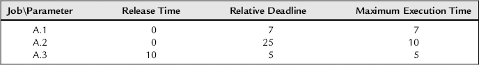

Figure 14-13: EDF example.
EDF is an optimal scheduling algorithm for independent, preemptable jobs, which means that if there is any algorithm that can produce a feasible schedule EDF will produce a schedule too. This seems like a very appealing algorithm to use, however we can say with a high level of probability that the RM algorithm is used much more frequently in practice. So, what are the reasons for this? There are several reasons and we will start with how this algorithm may be implemented using SmartDSP OS or SYS/BIOS.
As we saw before, RM or DM’s implementations are trivial as all DSP RTOSes support static priority scheduling and the above algorithms only show how the priorities are defined. Things are different for EDF. OS has to be able to change the priorities of a periodic job when it is released.
With SmartDSP, OS users can call the osTaskPrioritySet() function to adjust the priority. One important feature that the EDF algorithm requires is keeping FIFO for jobs in the same priority: for example, if task A is executing and task B is released so that at the release point the absolute deadlines are the same for both tasks. Task B should be put into the job queue and executed after A finishes. When we look at SmartDSP OS sources, we can see that in fact the following is what happens:
Function osTaskPrioritySet() will eventually call taskReadyAdd() for a task that its priority is set and it will call list_tail_add() putting task to the end of the list. So, from this perspective SmartDSP OS provides adequate implementation.
Another problem is that sometimes all priorities have to be remapped. Consider the following example [6]: “…consider the case in which two deadlines da and db are mapped into two adjacent priority levels and a new periodic instance is released with an absolute deadline dc, such that da <dc <db. In this situation, there is not a priority level that can be selected to map dc, even when the number of active tasks is less than the number of priority levels in the kernel. This problem can only be solved by remapping da and db into two new priority levels which are not consecutive. Notice that, in the worst case, all current deadlines may need to be remapped, increasing the cost of the operation.” This is especially true for SmartDSP OS as it has only 32 priorities and such remapping may happen relatively often.
With SYS/BIOS users can use the following function:
UInt Task_setPri(Task_Handle handle, Int newpri);
It will also add task to the end of the priority queue which is expected by EDF. Number of different priorities levels for SYS/BIOS is 32 for some platforms and 16 for others so in that sense it may require even more remapping than SmartDSP OS.
Another possible approach to take is to implement your own scheduler that will bypass scheduler of OS. For SYS/BIOS one possibility is to use negative priorities (−1) for all the tasks except the one that we want to execute. So, scheduler implementation could use EDF to determine the next task to run and then set its task’s priority to a non-negative number. The scheduler also can intercept task switches if required, using a hook. This mechanism may be required to be used when jobs use semaphores, as an example.
With SmartDSP OS it is possible to use osTaskActivate()/osTaskSuspend() pair to control a schedule from outside; however, there is no mechanism to control the context switch so a more complex scenario with EDF may not work.
To conclude the RTOS implementation topic, it may be challenging to implement EDF on top of existing RTOSes schedulers because they support a different paradigm that does not directly fit EDF.
This is not the only reason EDF did not find its way into many real-time DSP designs. Another problem with EDF is that it may produce less predictable results under high load. As [8] states, “The timing behavior of a system scheduled according to fixed-priority algorithm is more predictable than that of system scheduled according to dynamic-priority algorithm. When task have fixed priorities, overruns of jobs in task can never affect higher-priority tasks. It is possible to predict which tasks will miss their deadlines during an overload.”
Offline versus online scheduling
The difference between two types of scheduling is not as obvious as it seems at first glance. For both types of scheduling, users must perform offline research, at least related to schedulability of the jobs. As [10] states, “… we can conclude that the terms ‘offline’ and ‘online’ scheduling cannot be seen as disjointed in general. Real-time scheduling requires online guarantees, which require assumptions about online behavior at design time. At runtime, both offline and online execute according to some (explicitly or implicitly) defined rules, which guarantee feasibility. The question offline versus online is thus less black and white, but more about how much of the decision process is online. Thus, both offline and online are based on a substantial online part. The question is then where to set the tradeoff between determinism – all decisions online – and flexibility – some decisions online.”
Priority inversion
As we have mentioned before, one of the effects that prevent simple deployment of scheduling techniques is priority inversion. Priority inversion is defined as a situation where a lower priority job is executed in time when a higher priority job should run instead. According to this definition calls that disable scheduler (e.g., osTaskSchedulerLock() in SmartDSP OS or SYS/BIOS’ Task_disable()), disabling interrupts, utilizing semaphores or any other similar actions may cause priority inversion. Let’s look at a couple of examples of priority inversion starting with Figure 14-14.

Figure 14-14: Priority inversion.
In the above diagram A.1 job has higher priority than A.2. A.1 release time is 10 and A.2 is 0. Relative deadline and maximum execution time for A.1 are 15. Relative deadline for A.2 is 35 and maximum execution time is 20.
At time 0 job A.2 releases and begins executing.
At time 7 job A.2 acquires semaphore S.
At time 10 job A.1 releases and scheduler puts it to execution as one having higher priority.
At time 15 job A.1 tries to acquire semaphore S and as a result blocks and A.2 resumes.
At time 20 job A.2 releases semaphore S and A.1 resumes as it has higher priority.
At time 25 job A.1 misses its deadline and terminates (we assume here that the job terminates itself if it misses the deadline). Job A.2 resumes.
In this example, job A.1 misses its deadline as result of priority inversion that was in turn caused by resource contention. In such case the priority inversion was bound as A.2 kept the resource and continued execution and would eventually release the resource. It is important to mention that the same behavior would arise if an implementation used scheduler locking of any kind.
In Figure 14-15, the A.1 job is hard real time and it has highest priority. A.1 release time is 10, maximum execution time is 15 and relative deadline is 15. A.2 is a sporadic, non real-time job and it is released at 10 as well and is executed for 25. A.3 is a non real-time job too and it is released at 0.

Figure 14-15: Unbounded priority inversion.
The problem here is that a medium priority sporadic job is executing while a higher priority job is blocked by a low priority job holding mutually exclusive resources.
Until this point we have described the problem by providing some basic examples for it. For the first type of priority inversion that we have described (bounded case) there is no ‘magic’ algorithm to apply and the solutions may include:
• Shorten length of shared resource usage.
• Use a synchronization method that is the weakest possible. For example, if threads that contend for resources are implemented as tasks then use semaphores or disable the scheduler etc.
• Avoid resource sharing. In many cases it is possible to avoid resource sharing by proper usage of hardware and partitioning.
• Deploy virtualization techniques so that resources are virtualized thru some central entity and thus can be used in parallel.
Clearly, all these methods will help for an uncontrolled case as well, but for such a case there are some additional methods that can be deployed.
A very straightforward way is to use scheduler disabling methods as shown in Table 14-5.
Table 14-5: Multithreading disable API.

Disabling scheduler
The simplest way to resolve uncontrolled priority inversion is by disabling scheduling of the appropriate threading layer before task begins using shared resource. It is easy to see why it resolves any uncontrolled priority inversion: no other thread can start executing while the resource is used (that can be weakened to some extent. For example, if we know that HWI are short enough we can only lock tasks and SWI). This approach will work adequately when the time period for which the resource is utilized is relatively short; with longer periods of time another problem arises: bounded priority inversion relative to all threads in the system. So, we basically traded a possibility for uncontrolled priority inversion to a generally higher possibility of controlled priority inversion.
Priority inheritance
Another possible solution that is proposed by [7] is uses of the priority inheritance algorithm. The idea behind this algorithm is simple: when job A holds resource and higher priority job B tries to use it as well, A inherits B’s priority so it is able to complete its work with the resource. This approach has advantages over the previous one as tasks that have higher priority and do not contend over resources will preempt, while in the previous, simplistic approach this will not happen thus introducing additional priority inversion. Priority inheritance is often supported by OSes, for example, SYS/BIOS supports the priority inheritance algorithm with GateMutexPri module [18]: “To guard against priority inversion, GateMutexPri implements priority inheritance: when task High tries to acquire a gate that is owned by task Low, task Low’s priority will be temporarily raised to that of High, as long as High is waiting on the gate. Task High will ‘donate’ its priority to task Low. When multiple tasks wait on the gate, the gate owner will receive the highest priority of any of the tasks waiting on the gate.”
SmartDSP OS does not support priority inheritance directly. Some changes in API will be required if someone decides to implement this algorithm on top of existing API. For example, current API does not allow the getting of information on a pending task.
Priority ceiling
The inheritance algorithm does not resolve all possible issues (specifically when we consider several resources that need to be protected) such as deadlocks and may produce some timing anomalies [17] so a more sophisticated algorithm was introduced – the priority ceiling algorithm [7]. No DSP RTOS we looked at implemented this later algorithm.
Tools support for DSP OSes
Several types of tools exist today:
• Log visualization: tools visualizing an OS’s log.
• Context support in IDE: browsing thread’s variables.
• Configuration: visual configuration of OS supported modules, drivers, etc.
Let’s discuss all the above tools in more detail.
When you debug a race condition it is beneficial to see if some thread is preempted; when you try to find issues related to priority inversion, it is important to understand the timeline of different events that happen in the system in run-time. Hardware interrupts, scheduling events, context switches, and user-defined events are logged and then visualized (see Figure 14-16). It is also very useful and easy with this kind of tool to measure intervals between different events. The implementation of such a tool has two parts: logging that happens on the target and tool itself that can get this data from the target and visualize. Implementation on the target should be very effective and not intrusive as it should not affect normal execution of the program.

Figure 14-16: Log viewer.
SYS/BIOS’s tool that supports above functionality is System Analyzer [22]. Users can also add functionality on the target using UIA (the Unified Instrumentation Architecture) concepts. For example, to measure time between two calls using System Analyzer users can call:
Log_write1(UIABenchmark_start, (xdc_IArg)"user_thread_1");
And then:
Log_write1(UIABenchmark_stop, (xdc_IArg)"user_thread_1");
SmartDSP OS has a similar tool (see screenshot in Figure 14-17).

Figure 14-17: Graphic configuration tool.
Another important functionality that becomes important today is timeline correlation between different instances of OSes in an AMP system or even different OSes in heterogeneous systems (e.g., Linux and SYS/BIOS).
Sometimes you need to debug an OS with a source level debugger. With DSPs you will probably use a JTAG connection and some IDE. When RTOS is executing on target the IDE has to be aware of its existence so that it can show information correctly. For example, show variables that are local to specific context, and show program counters for different threads of execution.
Another aspect that is handled by visual tools sometimes is initial configuration. Such a tool can help to include a particular module for OS or to help to configure hardware.
Figure 14-17 shows a snapshot of tool that accompanies SmartDSP OS – CommExpert. This tool allows configuration of the OS and underlying hardware using graphical user interface.
Conclusions
Today’s DSP RTOSs have to support complex SoCs that may include several DSP cores, numerous peripherals that interact with external devices and networks, memory sub-systems that may have a few cache levels, bus or switch fabric, different types of memory with different accesses types, DMAs, or DSP co-processors. OSes have to abstract and encapsulate this complexity by proper partitioning layers of standard API to handle common functionality like DMA or Ethernet. Multicore platforms are still relatively new in the DSP world but we can already see how DSP RTOSs approach it: hardware resource partitioning, early multiplexing of network traffic, cooperative AMP, and well defined IPC are some of the most important features related to multicore.
On another front, scheduling of real-time jobs in such a complex environment still remains challenging and we can see that not all of those theoretical concepts that we have described made their way into RTOS’s code. As for the resource contention topics that we discussed, clearly, there are no mechanisms in existence today that can completely resolve resource contention-related anomalies, so we believe that the best way to resolve this is to avoid resource sharing, with proper partitioning or virtualization-like mechanisms.
REFERENCES
Refereed journal articles
1. Karam LJ, AlKamal I, Gatherer A, Frantz GA, Anderson DV, Evans BL. Trends in Multicore DSP Platforms. IEEE Signal Processing Magazine, Special Issue on Signal Processing on Platforms with Multiple Cores. Nov 2009;26(6):38–49.
2. Lee Edward A. What is ahead of embedded software?. Computer. Sep 2000;33(9):18–26.
3. C. Douglass Locke, Software architecture for hard real time applications: Cyclic Executives vs. Fixed Priority Executives, Real-time Systems, 4 (1) 37–53.
4. Liu CL, Layland JAMESW. Scheduling Algorithms for Multiprogramming in a Hard Real-Time Environment. Journal of the ACM (JACM). Jan 1973;20.
5. Leung JYT, Whitehead J. On the Complexity of Fixed-Priority Scheduling of Periodic, Real-Time Tasks. Performance Evaluation. 1982;2(4):237–250 December 1982.
6. Giorgio C. Buttazzo, Rate Monotonic vs. EDF: Judgment Day. Real-time Systems, 29 (1) 5–26.
7. Sha Lui. Ragunathan Rajkumar, John P Lehoczky Priority Inheritance Protocols: An Approach to Real-Time Synchronization. IEEE Transactions on Computers. Sep 1990;39(9):1175–1185.
Books and book chapters
8. Real-Time Systems, Prentice Hall, Publication Date: April 23, 2000. ISBN-13: 978-0130996510.
Refereed conference papers
9. Gerhard Fohler, Damir Isovi![]() , Tomas Lennvall, and Roger Vuolle. SALSART – AWeb Based Cooperative Environment for Offline Real-time Schedule Design, Proc. Parallel, Distributed and Network-based Processing, 2002, 10th Euromicro Workshop on Issue, 2002, pp. 63–70.
, Tomas Lennvall, and Roger Vuolle. SALSART – AWeb Based Cooperative Environment for Offline Real-time Schedule Design, Proc. Parallel, Distributed and Network-based Processing, 2002, 10th Euromicro Workshop on Issue, 2002, pp. 63–70.
10. Gerhard Fohler, University of Kaiserslautern, How Different are Offline and Online Scheduling? Proceedings of the 2nd International Real-Time Scheduling Open Problems Seminar, July 5, 2011, pp. 5–6, Beto, Portugal.
11. Young Michal. Lih-Chyun Shu Hybrid Online/Offline Scheduling for Hard Real-Time Systems. Proc 2nd International Symposium on Real-Time and Media Systems. 1996;231–240.
12. Audsley C, Burns A, Richardson MF, Wellings AJ. Hard Real-Time Scheduling: the Deadline-Monotonic Approach. Proc IEEE Workshop on Real-Time Operating Systems and Software 1991;133–137.
13. Lehoczky John, Sha Lui, Ding Ye. The Rate Monotonic Scheduling Algorithm: Exact Characterization and Average Case Behavior. Proc Real Time Systems Symposium 5–7 Dec 1989;166–171 Santa Monica, CA, USA.
14. E. Bini, G. Buttazzo, A hyperbolic bound for the rate monotonic algorithm, Proc. Real-Time Systems, 13th Euromicro Conference, 13 Jun 2001 – 15 Jun 2001, Delft, Netherlands, pp. 59–66.
Technical reports
15. Richard M. Karp, On-Line Algorithm Versus Off-Line Algorithm: How Much is it Worth to Know the Future?, International Computer Science Institute, Technical report TR-92-044.
16. Davis Robert I, Burns Alan. A Survey of Hard Real-Time Scheduling Algorithms and Schedulability Analysis Techniques for Multiprocessor Systems. 2011; http://www.cs.york.ac.uk/ftpdir/reports/2009/YCS/443/YCS-2009-443.pdf; 2011; Retrieved at 11.11.
17. Victor Yodaiken. Against priority inheritance. FSMLABS Technical Report September 23, 2004.
Product documentation
18. SYS BIOS API Documentation, Version bios_6_32_00_28.
19. TMS320C6000 Network Developer’s Kit (NDK) Software, TI Document identifier spru523g.
20. LINX Protocols, Document Version 21. http://linx.sourceforge.net/linxdoc/doc/book-linx-protocols.pdf. Retrieved 29.11.2011.
21. TIPC: Transparent Inter Process Communication Protocol http://tipc.sourceforge.net/doc/draft-spec-tipc-07.txt. Retrieved 29.11.2011.
22. System Analyzer User’s Guide, TI Literature Number: SPRUH43B. July 2011.
23. SYS/BIOS Inter-Processor Communication (IPC) and I/O User’s Guide, Literature Number: SPRUGO6C.
24. KeyStone Architecture Multicore Navigator, User Guide, TI Literature Number SPRUGR9D.
25. TMS320C66x DSP generation of devices, TI Literature Number SPRT580A.
26. SysLink User Guide, http://processors.wiki.ti.com/index.php/SysLink_UserGuide. Retrieved 29.11.2011.
27. MSC8156 Data Sheet, Freescale Semiconductor. Document Number: MSC8156, Rev. 4, 10/2011. http://www.freescale.com/webapp/sps/site/prod_summary.jsp?code=MSC8156. Retrieved 11.30.2011.