
Chapter 1
Introduction to Digital Signal Processing
Chapter Outline
What is digital signal processing?
Power efficient DSP applications
What is digital signal processing?
Digital signal processing (DSP) is the method of processing signals and data in order to enhance, modify, or analyze those signals to determine specific information content. It involves the processing of real-world signals that are converted to, and represented by, sequences of numbers. These signals are then processed using mathematical techniques, in order to extract certain information from the signal, or to transform the signal in some preferably beneficial way.
The term ‘digital’ in DSP requires processing using discrete signals to represent the data in the form of numbers that can be easily manipulated. In other words, the signal is represented numerically. This type of representation implies some form of quantization of one or more properties of the signal, including time.
This is just one type of digital data; other types include ASCII numbers and letters that have a digital representation as well.
The term ‘signal’ in DSP refers to a variable parameter. This parameter is treated as information as it flows through an electronic circuit. The signal usually starts out in the analog world as a constantly changing piece of information.1 Examples of real-world signals include:
The signal is essentially a voltage that varies among a theoretically infinite number of values. This represents patterns of variation of physical quantities. Other examples of signals are sine waves, the waveforms representing human speech, and the signals from a conventional television. A signal is a detectable physical quantity. Messages or information can be transmitted based on these signals.
A signal is called one dimensional (1-D) when it describes variations of a physical quantity as a function of a single independent variable. An audio/speech signal is one dimensional because it represents the continuing variation of air pressure as a function of time.
Finally, the term ‘processing’ in DSP relates to the processing of data using software programs as opposed to hardware circuitry. A DSP is a device or a system that performs signal processing functions on signals from the real (analog) world, primarily using software programs to manipulate the signals. This is an advantage in the sense that the software program can be changed relatively easily to modify the performance or behavior of the signal processing. This is much harder to do with analog circuitry.
Since DSPs interact with signals in the environment, the DSP system must be ‘reactive’ to the environment. In other words the DSP must keep up with changes in the environment. This is the concept of ‘real-time’ processing and we will talk about this shortly.
Advantages of DSP
There are many advantages of using a digital signal processing solution over an analog solution. These include:
• Changeability; it is easy to reprogram digital systems for other applications, or to fine tune existing applications. A DSP allows for easy changes and updates to the application.
• Repeatability; analog components have characteristics that may change slightly over time or temperature variances. A programmable digital solution is much more repeatable due to the programmable nature of the system. Multiple DSPs in a system, for example, can also run the exact same program and be very repeatable. With analog signal processing, each DSP in the system would have to be individually tuned.
• Size, weight, and power; a DSP solution that requires mostly programming means the DSP device itself consumes less overall power than a solution using all hardware components.
• Reliability; analog systems are reliable to the extent to which the hardware devices function properly. If any of these devices fail due to physical condition, the entire system degrades or fails. A DSP solution implemented in software will function properly as long as the software is implemented correctly.
• Expandability; to add more functionality to an analog system, the engineer must add more hardware. This may not be possible. Adding the same functionality to a DSP involves adding software, which is much easier.
DSP systems
The signals that a DSP processor uses come from the real world. Because a DSP must respond to signals in the real world, it must be capable of changing based on the changes it sees in the real world. We live in an analog world in which the information around us changes, sometimes very quickly. A DSP system must be able to process these analog signals and respond back to the real world in a timely manner. A typical DSP system (Figure 1-1) consists of the following:
• Signal source; something that is producing the signal such as a microphone, a radar sensor, or a flow gauge.
• Analog signal processing (ASP); circuitry to perform some initial signal amplification or filtering.
• Analog-to-digital conversion (ADC); an electronic process in which a continuously variable signal is changed, without altering its essential content, into a multi-level (digital) signal. The output of the ADC has defined levels or states. The number of states is almost always a power of two – that is, 2, 4, 8, 16, etc. The simplest digital signals have only two states, and are called binary.
• Digital signal processing (DSP); the various techniques used to improve the accuracy and reliability of modern digital communications. DSP works by clarifying, or standardizing, the levels or states of a digital signal. A DSP system is able to differentiate, for example, between human-made signals, which are orderly, and noise, which is inherently chaotic.
• Computer; if additional processing is required in the system, additional computing resources can be applied, if necessary. For example, if the signals being processed by the DSP are to be formatted for display to a user, an additional computer can be used to perform these tasks.
• Digital-to-analog conversion (DAC); the process in which signals having a few (usually two) defined levels or states (digital) are converted into signals having a theoretically infinite number of states (analog). A common example is the processing, by a modem, of computer data into audio-frequency (AF) tones that can be transmitted over a twisted pair telephone line.
• Output; a system for realizing the processed data. This may be a terminal display, a speaker, or another computer.

Figure 1-1: A DSP system.
Systems operate on signals to produce new signals. For example, microphones convert air pressure to electrical current, and speakers convert electrical current to air pressure.
Analog-to-digital conversion
The first step in a signal processing system is getting the information from the real world into the system. This requires transforming an analog signal to a digital representation suitable for processing by the digital system. This signal passes through a device called an analog-to-digital converter (A/D or ADC). The ADC converts the analog signal to a digital one by sampling or measuring the signal at a periodic rate. Each sample is assigned a digital code (Figure 1-2). These digital codes can then be processed by the DSP. The number of different codes or states is almost always a power of two (2, 4, 8, 16, etc.). The simplest digital signals have only two states. These are referred to as binary signals.

Figure 1-2: Analog-to-digital conversion for signal processing.
Examples of analog signals are waveforms representing human speech and signals from a television camera. Each of these analog signals can be converted to digital form using ADC and then processed using a programmable DSP.
Digital signals can be processed more efficiently than analog signals. Digital signals are generally well-defined and orderly which makes them easier for electronic circuits to distinguish from noise, which is chaotic. Noise is basically unwanted information. Noise can be anything from the background sound of an automobile engine, to a scratch on a picture that has been converted to digital format. In the analog world noise can be represented as electrical or electromagnetic energy that degrades the quality of signals and data. Noise, however, occurs in both digital and analog systems. Sampling errors (we’ll talk more about this later) can degrade digital signals as well. Too much noise can degrade all forms of information including text, programs, images, audio and video, and telemetry. Digital signal processing provides an effective way to minimize the effects of noise by making it easy to filter this ‘bad’ information out of the signal.
As an example, assume that the analog signal in Figure 1-2 needs to be converted into a digital signal for further processing. The first question to consider is how often to sample or measure the analog signal in order to represent that signal accurately in the digital domain. The sample rate is the number of samples of an analog event (like sound) that are taken per second to represent the event in the digital domain. Let’s assume that we are going to sample the signal at a rate of T seconds. This can be represented as:
Sampling period (T) = 1 / Sampling frequency (fs)
where the sampling frequency is measured in hertz (Hz).2
If the sampling frequency is 8 kilohertz (kHz), this would be equivalent to 8000 cycles per second. The sampling period would then be:
T = 1 / 8000 = 125 microseconds = 0.000125 seconds
This tells us that, for this signal being sampled at this rate, we would have 0.000125 seconds to perform all the processing necessary before the next sample arrived (remember, these samples arrive on a continuous basis and we cannot fall behind in processing them). This is a common restriction for real-time systems which we will discuss shortly.
If we now know the time restriction, we can then determine the processor speed required to keep up with this sampling rate. Processor speed is measured not by how fast the clock rate is for the processor, but how fast the processor executes instructions. Once we know the processor instruction cycle time, we can determine how many instructions we have available to process the sample:
Sampling period (T) / Instruction cycle time = number of instructions per sample
For a 100 MHz processor that executes one instruction per cycle, the instruction cycle time would be:
1/100MHz = 10 nano seconds
125 us / 10 ns = 12,500 instructions per sample
125 us / 5 ns = 25,000 instructions per sample (for a 200 MHz processor)
125 us / 2 ns = 62,500 instruction per sample (for a 500 MHz processor)
As this example demonstrated, the higher the processor instruction cycle execution, the more processing we can do on each sample. If it were this easy, we could just choose the highest processor speed available and have plenty of processing margin. Unfortunately, it is not as easy as this. Many other factors including cost, accuracy, and power limitations must also be considered. Embedded systems have many constraints such as these, as well as size and weight (important for portable devices). For example, how do we know how fast we should sample the input analog signal to accurately represent it in the digital domain? If we do not sample often enough, the information we obtain will not be representative of the true signal. If we sample too much, we may be ‘over-designing’ the system, and overly constraining ourselves.
The Nyquist criteria
One of the most important rules of sampling is called the Nyquist Theorem3, which states that the highest frequency which can be accurately represented is one-half of the sampling rate. The Nyquist rate specifies the minimum sampling rate that fully describes a given signal. Adhering to the Nyquist rate enables accurate reconstruction of the original signal from the samples. The actual sampling rate required to reconstruct the original signal must be somewhat higher than the Nyquist rate, because of various quantization errors introduced by the sampling process.
For example, human hearing ranges from 20 Hz to 20,000 Hz, so to imprint sound to a CD, the frequency must be sampled at a rate of 40,000 Hz to reproduce the 20,000 Hz signal. The CD standard is to sample 44,100 times per second, or 44.1 kHz.
If a signal is not sampled at the Nyquist rate, the data sampled will not accurately represent the true signal. Consider the sine wave below:
The dashed vertical lines are sample intervals. The dots are the crossing points on the signal. These represent the actual samples taken during the conversion process (for example, an analog-to-digital converter). If the sampling rate in Figure 1-3 is below the required Nyquist frequency, this causes a problem. If the signal is reconstructed, the resultant waveform, as shown in Figure 1-4, can occur.

Figure 1-3: A signal sampled at a rate below the Nyquist rate will not fully represent the true signal.
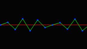
Figure 1-4: A reconstructed waveform showing the problem when the Nyquist theorem is not followed.
This signal looks nothing like the input. This undesirable feature is referred to as ‘aliasing’. Aliasing is the generation of a false (or alias) frequency, along with the correct one, when performing frequency sampling in a given signal.
Aliasing manifests itself differently, depending on the signal affected. Aliasing shows up images as a jagged edge or stair-step effect. Aliasing affects sound by producing a ‘buzz’. In order to reduce or eliminate this noise, the output from the ADC process is usually low-pass filtered to remove the higher frequency signals above the Nyquist frequency. Low-pass filtering also eliminates unwanted high-frequency noise and interference introduced prior to the sampling phase. We will talk more about filtering algorithms in coming chapters.
Let’s assume we want to convert an analog audio into a digital signal for further processing. We use the term ‘analog’ in an audio context to refer to a signal that represents sound waves traveling through the air. A simple audio tone, such as a sine wave, will cause the air to form evenly spaced ripples of alternating high and low pressure. When these signals enter a microphone (or an eardrum for that matter), they cause sensors to move evenly back and forth, at the same rate, producing a voltage. The measured voltage coming from the microphone, plotted over time, will look similar to that shown in Figure 1-5.

Figure 1-5: Analog data plotted over time.
If we want to edit, manipulate, or otherwise transmit this signal over a communication link, the signal must be digitized first. The incoming analog voltage levels are converted into binary numbers using analog-to-digital conversion. The two important constraints when performing this operation are sampling frequency (how often the voltage is measured) and resolution (the size of digital numbers used to measure the voltage, specifically the size or width of the A/D converter.
Larger ADCs allow for an increased dynamic range of the input signal. When an analog waveform is digitized we are essentially taking continuous ‘snapshots’ of the waveform at a certain interval, called the sampling frequency, and storing those snapshots as binary codes or numbers.
When the waveform is reconstructed from the sequence of numbers, the result will be a ‘stair-step’ approximation of what we started with (Figure 1-6).

Figure 1-6: Resultant analog signal reconstructed from the digitized samples.
To convert this digital data back into analog voltages, the stair-step approximation must be ‘smoothed’ using a filter. This will produce an output similar to the input (assuming no additional processing has been performed). However, if the sampling frequency, signal resolution, or both, are too low, the reconstructed waveform will be of lower quality. Failing to process a signal at the sample rate (or higher) is as bad as a miscalculation in a hard real-time system such as a CD player. This can be generalized to:
(Number of instructions to process ∗ Sample rate) < Fclk ∗ Instructions/cycle (MIPS)
where Fclk is the clock frequency of the DSP device.
The required sampling rate depends on the application. There is a wide range of sampling rates, from radar and signal processing applications on the high end, where the sampling rate may be up to 1 gigahertz and beyond to control and instrumentation which require a much lower sampling rate, in the order of 10 to 100 hertz. Algorithm complexity must also be taken into consideration. In general, the more complex the algorithm, the more instruction cycles are required to compute the result, and the lower the sampling rate must be to accommodate the time for processing these complex algorithms.
Digital-to-analog conversion
In many applications, a signal must be sent back out to the real world after being processed, enhanced and/or transformed while inside the DSP. Digital-to-analog conversion (DAC) is a process in which digital signals having a few (usually two) defined levels or states are converted into analog signals having a very large number of states.
Both the DAC and the ADC are of significance in many applications of digital signal processing. The fidelity of an analog signal can often be improved by converting the analog input to digital form using a DAC, clarifying or enhancing the digital signal, and then converting the enhanced digital impulses back to analog form using an ADC (a single digital output level provides a DC output voltage).
Figure 1-7 shows a digital signal passing through a digital-to-analog (D/A or DAC) converter which transforms the digital signal into an analog signal and outputs that signal to the environment.

Figure 1-7: Digital-to-analog conversion.
Applications for DSPs
In this section, we will explore some common applications for DSPs. Although there are many different DSP applications, I will focus on three categories:
Low cost DSP applications
DSPs are becoming an increasingly popular choice as low cost solutions in a number of different areas. One popular area is electronic motor control. Electric motors exist in many consumer products, from washing machines to refrigerators. The energy consumed by the electric motor in these appliances is a significant portion of the total energy consumed by the appliance.
Controlling the speed of the motor has a direct effect on the total energy consumption of the appliance. In order to achieve the performance improvements necessary to meet energy consumption targets for these appliances, manufacturers use advanced three-phase variable speed drive systems. DSP-based motor control systems have the bandwidth required to enable the development of more advanced motor drive systems for many domestic appliance applications.
Application complexity has continued to grow as well, from basic digital control to advanced noise and vibration cancellation applications. As the complexity of these applications has grown, there has also been a migration from analog-to-digital control. This has resulted in an increase in reliability, efficiency, flexibility, and integration, leading to overall lower system costs.
Many of the early control functions used what is called a microcontroller as the basic control unit. As the complexity of the algorithms in motor control systems increased, the need also grew for higher performance and more programmable solutions. Digital signal processors provide much of the bandwidth and programmability required for such applications. DSPs are now finding their way into some of the more advanced motor control technologies:
• Variable speed motor control
• Improvements in control algorithms
• Replacement of costly hardware components with software routines
Motor control is one example of a low cost DSP application. In this example, the DSP is used to provide fast and precise PWM switching of the converter. The DSP also provides the system with fast, accurate feedback of the various analog motor control parameters such as current, voltage, speed, temperature, etc. There are two different motor control approaches; open-loop control and closed-loop control. The open-loop control system is the simplest form of control. Open-loop systems have good steady state performance and the lack of current feedback limits much of the transient performance. A low cost DSP is used to provide variable speed control of the three-phase induction motor, providing improved system efficiency.
A closed-loop solution is more complicated. A higher performance DSP is used to control current, speed, and position feedback, which improves the transient response of the system and enables tighter velocity/position control. Other, more sophisticated, motor control algorithms can also be implemented in the higher performance DSP.
There are many other applications using low cost DSPs. Refrigeration compressors, for example, use low cost DSPs to control variable speed compressors which dramatically improve energy efficiency. Low cost DSPs are used in many washing machines to enable variable speed control, which has eliminated the need for mechanical gearing. DSPs also provide sensorless control for these devices, which eliminates the need for speed and current sensors. Improved off-balance detection and control enable higher spin speeds, which get clothes dryer with less noise and vibration. Heating, ventilating, and air conditioning (HVAC) systems use DSPs in variable speed control of the blower and inducer, which increases furnace efficiency and improves comfort.
Power efficient DSP applications
We live in a portable society. From cell phones to personal digital assistants (PDAs), we work and play on the road! These systems are dependent on the batteries that power them. The longer the battery life can be extended, the better. So it makes sense for the designers of these systems to be sensitive to processor power. Having a processor that consumes less power enables longer battery life, and makes these systems and applications possible.
As a result of reduced power consumption, systems dissipate lower heat. This results in the elimination of costly hardware components like heat sinks to dissipate the heat effectively. This leads to overall lower system cost, as well as smaller overall system size, because of the reduced number of components. Continuing along this same line of reasoning, if the system can be made less complex with fewer parts, designers can bring these systems to market more quickly.
Low power devices also give the system designer a number of new options, such as potential battery back-up to enable uninterruptible operation, as well as the ability to do more with the same power (as well as cost) budget, to enable greater functionality and/or higher performance.
There are several classes of systems that are suitable for low power DSPs. Portable consumer electronics use batteries for power. Since the average consumer of these devices wants to minimize the replacement of batteries, the longer they can go on the same batteries, the better off they are. This class of customer also cares about size. Consumers want products they can carry with them, clip onto their belts, or carry in their pockets.
Certain classes of system require designers to adhere to a strict power budget. These include those that have a fixed power budget, such as systems that operate on limited line power, battery back-up, or with a fixed power source. For these classes of systems, designers aim to deliver functionality within the constraints imposed by the power supply. Examples include many defense and aerospace systems. These systems also have very tight size, weight, and power restrictions. Low power processors give designers more flexibility under all three of these important constraints.
Another important class of power-sensitive systems include high density systems. These systems are often high performance, or multi-processor systems. Power efficiency is important for these types of systems, not only because of the power supply constraints, but also because of heat dissipation concerns. These systems contain very dense boards with a large number of components per board. There may also be several boards per system in a very confined area. Designers of these systems are concerned about reduced power consumption, as well as heat dissipation. Low power DSPs can lead to higher performance and higher density. Fewer heat sinks and cooling systems enable lower cost systems that are easier to design. The main concerns for these systems are:
• Creating more functions per channel
• Achieving more functions per square inch
Power is the limiting factor in many systems today. Designers must optimize the system design for power efficiency at every step. One of the first steps in any system design is the selection of the processor. A processor should be selected based on an architecture and instruction set optimized for power efficient performance. For signal processing intensive systems, a common choice is a DSP.
As an example of a low power DSP solution, consider a solid state audio player. This system requires a number of DSP-centric algorithms to perform the signal processing necessary to produce high fidelity quality music sound. A low power DSP can handle the decompression, decryption, and processing of audio data. This data may be stored on external memory devices which can be interchanged like individual CDs. These memory devices can be reprogrammed as well. The user interface functions can be handled by a microcontroller. The memory device which holds the audio data may be connected to the micro which reads it and transfers it to the DSP. Alternatively, data might be downloaded from a PC or internet site and played directly, or written onto blank memory devices. A digital-to-analog (DAC) converter translates the digital audio output of the DSP into an analog form to eventually be played on user headphones. The entire system must be powered from batteries, (for example, two AA batteries).
For this type of product, a key design constraint would be power. Customers do not like replacing the batteries in their portable devices. Thus, battery life, which is directly related to system power consumption, is a key consideration. By not having any moving parts, a solid state audio player uses less power than previous generation players (such as tapes and CDs). Since this is a portable product, size and weight are obviously also key concerns. Solid state devices, such as the one described here, are also size efficient because they contain fewer parts in the overall system.
To the system designer, programmability is a key concern. With a programmable DSP solution, this portable audio player can be updated with the newest decompression, encryption, and audio processing algorithms instantly from the world wide web, or from memory devices. A low power DSP-based system solution like the one described here could have system power consumption as low as 200mW. This will allow the portable audio player to have three times the battery life of a CD player on the same two AA battery supply.
High performance DSP applications
At the high end of the performance spectrum, DSPs utilize advanced architectures to perform signal processing at high rates. Advanced architectures such as Very Long Instruction Word (VLIW) use extensive parallelism and pipelining to achieve high performance. These advanced architectures take advantage of other technologies, such as optimizing compilers, to achieve this performance. There is a growing need for high performance computing. Applications include:
Conclusion
Though analog signals can also be processed using analog hardware (i.e., electrical circuits containing active and passive elements), there are several advantages to digital signal processing:
• Analog hardware is usually limited to linear operations; digital hardware can implement nonlinear operations.
• Digital hardware is programmable, which allows for easy modification of the signal processing procedure in both real-time and non real-time modes of operation.
• Digital hardware is less sensitive than analog hardware to variations such as temperature.
These advantages lead to lower cost, which is the main reason for the ongoing shift from analog to digital processing in wireless telephones, consumer electronics, industrial controllers, and numerous other applications.
The discipline of signal processing, whether analog or digital, consists of a large number of specific techniques. These can be roughly categorized into two families:
• Signal-analysis/feature-extraction techniques which are used to extract useful information from a signal. Examples include speech recognition, location, and identification of targets from radar signals, and detection and characterization of changes in meteorological or seismographic data.
• Signal filtering/shaping techniques which are used to improve the quality of a signal. Sometimes this is done as an initial step before analysis or feature extraction. Examples of these techniques include the removal of noise and interference using filtering algorithms, separating a signal into simpler components, and other time- and frequency-domain averaging.
A complete signal processing system usually consists of many components and incorporates multiple signal processing techniques.
1 Usually because some signals may already be in a discrete form. An example of this would be a switch which is represented discretely as being either open or closed.
2 Hertz is a unit of frequency (of change in state or cycle in a sound wave, alternating current, or other cyclical waveform) of one cycle per second. The unit of measure is named after Heinrich Hertz, the German physicist.
3 Named in 1933 after scientist Harry Nyquist.