ALL DATA IN DW 2.0—RELATIVE TO TIME

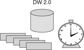
Figure 11.1 shows that all data in DW 2.0 is relative to time.

This fact means that when you access any given unit of data, you need to know at what time the data is accurate. Some data will represent facts from 1995. Other data will represent information from January. And other data will represent data from this morning.

In DW 2.0 then, whether it is explicit or implicit, all data has a moment in time that depicts its accuracy and relevancy. The data structure at the record level that is commonly used to make this depiction is seen by Figure 11.2.

In Figure 11.2 there are two record types. One record type is used for a snapshot of data at a single moment in time. This record type—on the left—has DATE and TIME as part of the key structure. The other type of record is shown on the right. It is a record that has a FROM date and a TO date. The implication is that a block of time—not a point in time—is being represented.

FIGURE 11.1 In one way or another, all data in the DW 2.0 environment is relative to time.

FIGURE 11.2 Time shows up as part of the key structure of the data.

FIGURE 11.3 In the Interactive Sector, data is correct as of the moment of usage.

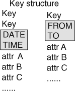
Note that in both cases the element of time is part of the key structure. The key is a compound key and the date component is the lower part of the compound key.

TIME RELATIVITY IN THE INTERACTIVE SECTOR

In the Interactive Sector, the time relevancy of data is somewhat different. In this sector, data values are assumed to be current as of the moment of access. For example, suppose you walk into a bank and inquire as to your balance in an account. The value that is returned to you is taken to be accurate as of the moment of access. If the bank teller says to you that you have $3971 in the bank, then that value is calculated up to the moment of access. All deposits and all withdrawals are taken into account.

Therefore, because interactive data is taken to mean accurate as of the moment of access, there is no date component to interactive data.

Figure 11.3 shows a banking transaction occurring in which interactive, up-to-the-second data is being used.

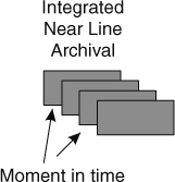
But in all other sectors of DW 2.0—in the Integrated Sector, the Near Line Sector, and the Archival Sector—data explicitly has a moment in time associated with the data.

DATA RELATIVITY ELSEWHERE IN DW 2.0

Figure 11.4 shows that each record in the Integrated Sector, the Near Line Sector, and the Archival Sector represents either a point in time or a span of time.

FIGURE 11.4 In all other sectors of DW 2.0, each record represents a moment in time.

FIGURE 11.5 In the Interactive Sector, the value of data is changed as a result of an activity.

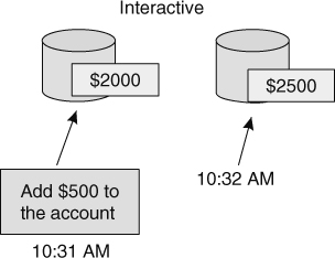
This notion of data being relative to time produces some very different ways of doing processing. In the interactive environment, update of data is done. In this case the update of data refers to the actual changing of the value of data. Figure 11.5 shows that a banking transaction is done and the value of the data is changed in the interactive environment.

At 10:31 AM there is $2000 in an account. A transaction adding $500 to the account occurs. The transaction is executed against the data in the data base and at 10:32 AM, the bank account has a balance of $2500.

The data has changed values because of the transaction.

TRANSACTIONS IN THE INTEGRATED SECTOR

Now let us consider a similar scenario in the Integrated Sector. At 10:31 AM there is a value of $2000 sitting in the integrated data base. A transaction is executed. At 10:32 a new record is placed in the data base. Now there are two records in the data base showing the different data at different moments in time.

FIGURE 11.6 In the Integrated Sector, a historical record is kept for all activities.

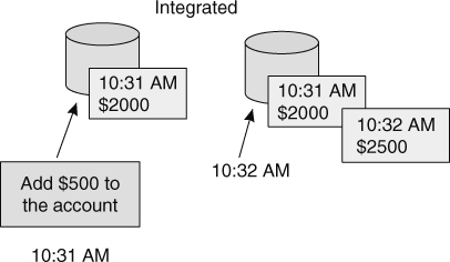
Figure 11.6 shows the execution of a transaction in the Integrated Sector.

The different data found in Figures 11.5 and 11.6 make it clear that because of the difference in the way data relates to time, the content of data in the different environments is very different.

There are terms for these different types of data. Figure 11.7 shows those terms.

FIGURE 11.7 The two common forms of time-variant data.

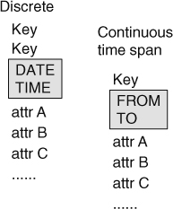
Where there is just a point in time, the data is called discrete data. Where there is a FROM date and a TO date, the data is called continuous time span data.

These two types of data have very different characteristics.

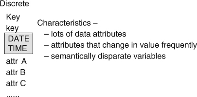
DISCRETE DATA

Discrete data is good for lots of variables that quickly change. As an example, consider the Dow Jones Industrial average. The Dow Jones is typically measured at the end of the day, not when a stock that is part of the Dow is bought or sold. The variables that are captured in the discrete snapshot include variables that are measured at the same moment in time. Other than that one coincidence, there is nothing that semantically ties the attributes of data to the discrete record.

Figure 11.8 shows some of the characteristics of the discrete structuring of data.

CONTINUOUS TIME SPAN DATA

Continuous time span data has a different set of characteristics. Typically, continuous time span data has very few variables in the record. And the variables that are in the record do not change often. The reason for these characteristics is that a new continuous time span record must be written every time a value changes. For example, suppose that a continuous time span record contains the following attributes:

Name

Address

Gender

Telephone Number

FIGURE 11.8 Some characteristics of discrete time-variant data.

A new record must be written every time one of these values changes. Name changes only when a woman marries or divorces, which is not often. Address changes more frequently, perhaps as often as every 2 to 3 years. Gender never changes, at least for most people. Telephone Number changes with about the same frequency as Address changes. Thus it is safe to put these attributes into a continuous time span record.

Now consider what would happen if the attribute Job Title were put into the record. Every time the person changed jobs, every time the person was promoted, every time the person transferred jobs, every time there was a corporate reorganization, it is likely that Job Title would change. Unless there were a desire to create many continuous time span records, it would not be a good idea to place Job Title with the other, more stable, data.

Figure 11.9 shows some of the characteristics of the continuous time span records.

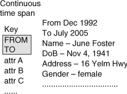
Great care must be taken in the design of a continuous time span record because it is possible to create a real mess if the wrong elements of data are not laced together properly. As a simple example, Figure 11.10 shows some typical attributes that have been placed in a continuous time span record.

FIGURE 11.9 Some characteristics of continuous time span time-variant data.

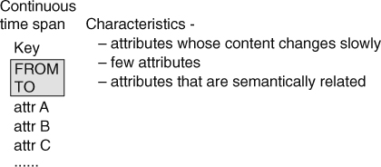
Figure 11.10 shows that the attributes Name, Date of Birth, Address, and Gender have been placed in a continuous time span record. These elements of data are appropriate because

they are slow to change in terms of content;

they all relate to descriptive information about an individual.

FIGURE 11.10 The implications of a continuous time span record.

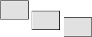
Whereas a single continuous time span record is useful, multiple continuous time span records can be strung together to logically form a much bigger record of continuity. Figure 11.11 shows several continuous time span records strung together.

FIGURE 11.11 A series of records are combined to form a continuous record over time.

A SEQUENCE OF RECORDS

The records form a continuous sequence. For example, one record ends on January 21, 2007, and the next record begins on January 22, 2007. In doing so, the records logically form a continuous set.

As a simple example, June Foster’s address was on Yelm Highway until July 20, 2002. One record indicates that value. Then June moved to Apartment B, Tuscaloosa, Alabama, and her official move date was July 21, 2002. A new record is formed. Together the two records show the date and time of her change of addresses and show a continuous address wherever she was at.

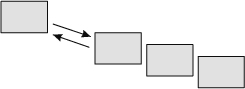
Although continuous time span records are allowed to form a continuous record, they are not allowed to overlap. If there were an overlap of records, there would be a logical inconsistency. For example, if two records had address information for June Foster and they overlapped, they would show that June lived in two places at once.

NONOVERLAPPING RECORDS

Figure 11.12 shows that continuous time span record overlap is not allowed.

FIGURE 11.12 Overlapping records are not allowed.

Although continuous time span records are not allowed to overlap, there can be periods of discontinuity. In 1995, June Foster sailed around the world. During that time she had no mailing address. The records of her address would show an address up until the moment she sailed and would show an address for her when she returned from her sailing voyage, but while she was on the voyage, there was no permanent address for her.

Figure 11.13 shows that gaps of discontinuity are allowed if they match the reality of the data.

FIGURE 11.13 Undefined gaps of time are allowed.

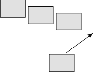
When it comes to adding new records, the new record is added as of the moment in time when the business was transacted or concluded. Depending on how the records are constructed, it may be necessary to adjust the ending record.

Figure 11.14 shows the update of a new record into a sequence of continuous records.

FIGURE 11.14 When it comes time to update a set of time span records, a new record is added.

BEGINNING AND ENDING A SEQUENCE OF RECORDS

There are a variety of options for beginning and ending the sequence of continuous time span records.

For example, suppose that the most current record is from May 1999 to the present. Suppose there is an address change in April 2007. A new record is written whose FROM date is April 2007. But to keep the data base in synch, the previous current record has to have the TO date adjusted to show that the record ends on March 2007.

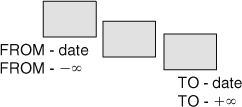
To that end, a sequence of records can begin and end anywhere. The FROM date for the first record in the sequence may have an actual date. Or the FROM date may be minus infinity. When the FROM date is minus infinity, the implication is that the record covers data from the beginning of time. Where there is a FROM date specified for the first record in a sequence, for any time before the FROM date, there simply is no definition of the data.

The ending sequence operates in much the same manner. The ending record in a continuous time span sequence may have a value in the TO field, or the TO value may be plus infinity. When the value is plus infinity, the implication is that the record contains values that will be applied until such time as a new record is written.

For example, suppose there is a contract whose TO value is plus infinity. The implication is that the contract is valid until such time as notification is given that the contract is over.

Figure 11.15 shows some of the options for starting and stopping a sequence of continuous time span records.

FIGURE 11.15 There are several options for start date and stop date.

CONTINUITY OF DATA

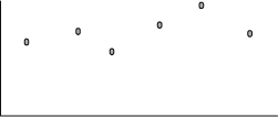
One of the limitations of discrete data is that there is no continuity between two measurements of data. For example suppose the NASDAQ closes at 2540 on Monday and at 2761 on Tuesday. Making the assumption that the NASDAQ was at a high of 2900 sometime on Tuesday is an assumption that cannot be made. In fact, no assumptions about the value of the NASDAQ can be made, other than at the end of the day when the measurements are made.

Figure 11.16 shows the lack of continuity of the discrete measurements of data.

FIGURE 11.16 With discrete data, there are no implications of continuity.

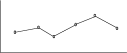
Continuous time span data does not suffer from the same limitations. With continuous time span data you can make a judgment about the continuity of data over time.

Figure 11.17 shows the continuity of data that can be inferred with continuous time span data.

FIGURE 11.17 With continuous time span data, there are definitely implications of continuity.

Whereas discrete data and continuous time span data are the most popular forms of data, they are not the only forms of time-variant data in DW 2.0. Another form of time-variant data is time-collapsed data.

TIME-COLLAPSED DATA

Figure 11.18 shows a simple example of time-collapsed data.

In time-collapsed data, there are several forms of measurement of data. When data enters the system it is measured in hours. Then at the end of the day, the 24 hours are added up to produce a recording of a day’s worth of activities. The 24-hour measurements are then reset to zero. At the end of a week, the week’s totals are created. Then the daily totals are reset to zero. At the end of the month, the month’s totals are created. Then the weekly totals are reset to zero. At the end of the year, the year’s totals are created. Then the monthly totals are reset to zero.

FIGURE 11.18 Time-collapsed data—another form of time-variant data.

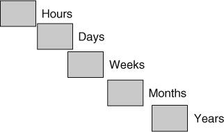
When this is done there is only one set of hourly totals, one set of daily totals, one set of weekly totals, and so forth. There is a tremendous savings of space.

The collapsing of time-variant data works well on the assumption that the fresher the data the more detail there needs to be. In other words, if someone wants to look at today’s hourly data, they can find it readily. But if someone wants to find hourly data from 6 months ago, they are out of luck.

In many cases the assumptions hold true and collapsing of data makes sense. But where the assumptions do not hold true, then collapsing data produces an unworkable set of circumstances.

TIME VARIANCE IN THE ARCHIVAL SECTOR

The last place where time variance applies to the DW 2.0 environment is in the Archival Sector. It is a common practice to store data by years. One year’s worth of data is stored, then another year’s worth of data is stored. There are many good reasons for the segmentation of data in this way. But the best reason is that the semantics of data have the habit of varying slightly each year.

One year a new data element is added. The next year a data element is defined differently. The next year a calculation is made differently. Each year is slightly different from each preceding year.

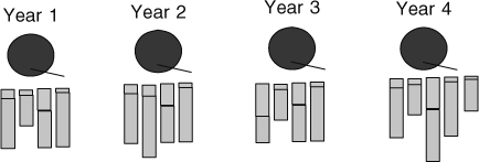
Figure 11.19 shows that each year there are slight changes to the semantics of data.

FIGURE 11.19 Archival data is stored on a year-by-year basis. Note that the data from one year to the next is never quite the same semantically.

FROM THE PERSPECTIVE OF THE END USER

Time variance is natural and normal to the business user of DW 2.0. When a business user wishes to look for data that is related to a moment in time, the end user supplies the time as a natural part of the analytic processing.

And when a business user wishes to look for the most current data, no date is supplied and the system understands that it needs to look for the most current unit of data.

So from the standpoint of a query and business user interaction, time variance is as normal and natural as making the query itself.

The business user is endowed with far greater analytical possibilities in DW 2.0 than he/she ever was in a previous environment.

The structure of DW 2.0 may require the end user to be aware that data of a certain vintage resides in one part of the DW 2.0 environment or the other. DW 2.0 may require separate queries for archival processing and against integrated data, for example.

However, the business user enjoys the benefits of performance that are gained by removing older, dormant data from the Integrated Sector. So there is a trade-off for sectoring data in DW 2.0.

SUMMARY

In one form or another, all data in DW 2.0 is relative to some moment in time.

Interactive data is current. It is accurate as of the moment of access. Other forms of data in DW 2.0 have time stamping of the record.

Time stamping takes two general forms. There is data that has a date attached. Then there is data that has a FROM and a TO field attached to the key. The first type of data is called discrete data. The second type is called continuous time span data.

Continuous time span data can be sequenced together over several records to form a long time span. The time span that is defined by continuous time span records can have gaps of discontinuity. But there can be no overlapping records.

There are other forms of time relativity in the DW 2.0 environment. There is time-collapsed data. Time-collapsed data is useful when only current data needs to be accessed and analyzed in detail. Over time the need for detail diminishes.

The other form of time relevancy in the DW 2.0 environment is that of archival data. As a rule archival data is organized into annual definitions of data. This allows for there to be slight semantic changes in data over time.