5

ADVANCED AND SELF-ADAPTING METHODS OF FREQUENCY-TO-CODE CONVERSION

In spite of the fact that today frequency can be measured by the most precise methods by comparison with other physical quantities, precise frequency-to-code conversion with the constant quantization error in a wide specified measuring frequency range (from 0.01 Hz up to some MHz) and with non-redundant conversion time can only be realized based on novel measurement methods for frequency-time parameters of the electric signal. This requires additional hardware costs and arithmetic operations: multiplication and division for calculations of the final result of conversion. Therefore, additional measuring (conversion) devices should be included in the microsystem. These include two or more multidigital binary counters, the multiplier and the code divider, logic elements, etc. Different design approaches are used. In the authors’ opinion, a successful solution is the use of a microcontroller core in such microsystems. In this case, with the aim to minimize the built-in hardware, it is expedient to take advantage of the program-oriented methods of measurement developed for frequency-time parameters of signals.

5.1 Ratiometric Counting Method

We shall first consider the idea of the original method of the discrete count [98,117], called the ratiometric counting method, which allows frequency-to-code conversion with a small constant error in a wide frequency range, we shall then consider how this method can be realized.

Let's assume that the converted periodic signal is in the form of sine wave. By means of the input forming device it will be transformed into a periodic sequence of pulses, the period T_x of which is equal to the period of the converted signal. There are various devices and principles for the transformation of periodic continuous signals into a sequence of rectangular pulses. For the practical usage, we provide a simple enough circuit of such an input shaper (Figure 5.1). It has an input voltage range from +0.035 up to +24 V. The device includes an input amplitude limiter, an amplifier and a Schmitt trigger.

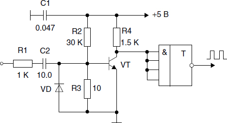
Figure 5.1 Circuit of input forming device

Regardless of this sequence the first reference time interval (gate time) T₀₁ is formed (Figure 5.2). It is filled out by N₁ pulses of the periodic sequence. The number N₁ is accumulated in the first counter. The converted frequency f′_x is determined according to the following

The frequency deviation from the value f_x is determined by the quantization error, the reduction of which is the aim of this method.

Simultaneously, the second gate time T₀₂, is formed. Its wavefront coincides with the pulse, appearing right after the start of the first gate time T₀₁, and the wavetail, with the pulse appearing right after the end of the first gate time T₀₁. Thus, the duration of the second gate time T₀₂ is precisely equal to the integer of the periods of the converted signal, i.e.

The wavefront and the wavetail of the formed gate time are synchronized with the pulses of the periodic input sequence generated from the input signal, therefore the rounding error is excluded. The second gate time is filled out by pulses of reference frequency f₀, whose number is accumulated in the second counter.

The formula for the calculation of the converted frequency can be obtained in the following way. The number of pulses which have got into the second gate time, as can be seen from Figure 5.2, is determined by the ratio

hence

where f₀ is the reference frequency. This can be done in a PC or a microcontroller core along with the offsetting and scaling that must often be performed.

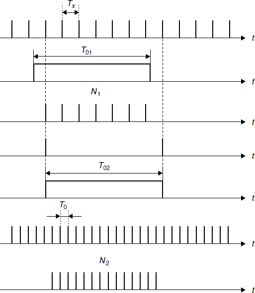
Figure 5.2 Time diagrams of ratiometric counting method

The accuracy of the frequency measurement is determined by the quantization error of the time interval N₁T_x.

Let's withdraw the equation for the relative quantization error δ_q for the frequency-to-code conversion. First of all we shall determine the maximum value of the relative quantization error for the time interval T₀₂ = N₁T_x. As this interval is filled out by counting pulses with the period T₀, the maximum absolute error is Δ₂ = ±T₀, and the maximum relative error is:

The equality N₁T_x = T₀₂ can be presented as f_x = N₁/T₀₂. Then according to the rules of the error calculation for indirect measurements the measurement error of the function f_x is connected with the measurement error of the argument T₀₂ by the ratio (with the accuracy of the second order of smallness) δ_q = δ₂. After substitution of δ₂ from Equation (5.5) we have:

According to the standard direct counting method it is possible to write the equality T₀₁ = N₁/f′_x. Substituting the relation f′_x/N₁ = 1/T₀₁, into Equation (5.6) instead f_x/N₁ we obtain:

This formula let us draw the conclusion that the maximum value of the relative quantization error for the frequency-to-code conversion for this method does not depend on converted frequencies and, hence, is constant in all conversion ranges of frequencies.

For a reference frequency f₀ = 1 MHz and the first gate time T₀₁ = 1 s the maximum value of the relative quantization error will be δ_q = ±10⁻⁴%.

If, by the measurement of the time interval T₀₂ = N₁T_x using the interpolation method considered in Chapter 4 with the same frequency and gate time we obtain δ_q = ±10⁻⁷%.

Equation (5.7) is suitable for engineering calculations. However, this equation is a simplified mathematical model. Its construction was based on two assumptions. In order to research limiting metrological characteristics of the method it is necessary to use the refined mathematical model of the quantization error [118].

In the common case, the number of pulses which have got into the second reference time interval T₀₂ (Figure 5.2), is unequivocally connected to the phase crowding of reference frequency fluctuations during the time τ = N₁T_x, expressed through 2π:

where ω₀ is the radian reference frequency; ent { } is the integer part of a number. Omitting the ent, we have:

On the other hand, on the strength of formula for T₀₂, it is possible to write down

This formula represents the refined mathematical model for the quantization error and can be used for frequency-to-code converter simulation for studying limiting metrological characteristics.

The graph of δ_q, T₀₂ against f_x is shown in Figure 5.3 and the functional relationship δ_q(f_x, T₀₁) in Figure 5.4. Functions δ_q = f(f_x), δ_q(f_x, T₀₁) and T₀₂ = ϕ(f_x) have the finite discontinuity of the first kind. As the modelling results show, the quantization error in the neighbourhood of the point f_{x min} is two times less than that calculated according to Equation (5.7). Thus, the second reference time interval T₀₂ is increased by as many times.

Finally, we consider the block diagram of the converter (Figure 5.5), which realizes the frequency-to-code conversion according to the considered ratiometric counting method.

It contains two counters and a D-trigger clocked with the sensor output. All counter functions can be provided by the counter/timer peripheral component, which interfaces to many popular microcontrollers.

Figure 5.3 Graph of δ_q(a) and T₀₂(b) against f_x at T₀₁ = 0.25 s and f₀ = 133 333.33 Hz

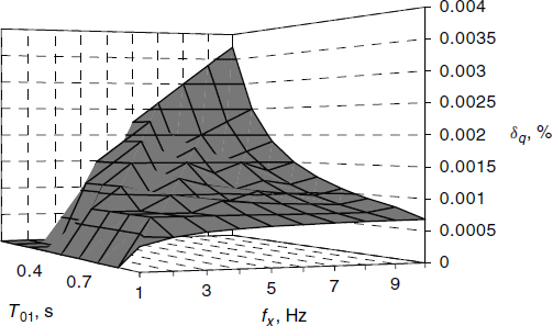
Figure 5.4 Graph of δ_q against f_x and T₀₁ at f₀ = 133 333.33 Hz

Figure 5.5 Ratiometric simplified counting scheme

This method can also be used for the period (T_x)-to-code conversion. Thus, the period is calculated according to the following formula

The main demerit of the considered conversion method is the redundant conversion time.

5.2 Reciprocal Counting Method

A variation of the method described above is the reciprocal counting method (Figure 5.6). The cyclicity of the conversion T_cycle is determined by the reset pulse. The beginning of the counting interval T_count coincides with the next pulse of sequence f_x, appearing after the ending of the ‘Start’ pulse, and the end coincides with the next pulse f_x, appearing after the ‘End’ pulse [105]. The frequency is calculated during the interval T_calc.

The frequency or the period are calculated similarly as described above according to Equations (5.4) and (5.11) accordingly. The quantization error is calculated according to the following:

However, in this method, the value of the first gate time T_count can be determined only approximately. Having set the conversion cycle equal to 1 s, it is possible to assume only that s. It is slightly inconvenient for engineering calculations of the quantization error δ_q.

This method has the same demerit as the ratiometric counting method–the redundant conversion time.

5.3 M/T Counting Method

The so-called M/T counting method, which also overcomes demerits of conventional methods (standard direct counting and indirect counting methods) and achieves high resolution and accuracy for a short detecting time was described in [110].

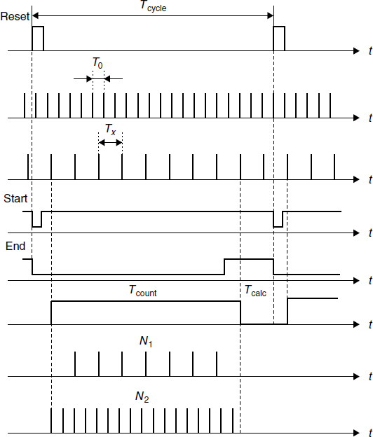
Figure 5.6 Time diagrams of reciprocal counting method

Time diagrams of the M/T counting method are shown in Figure 5.7. The detecting time T₀₂ is determined by synchronizing the generated output pulse after a prescribed period of time T₀₁.

It is easy to notice that the M/T method differs from the above described ratiometric counting method by the synchronization of the first reference time interval T₀₁ with the pulse of the converted frequency f_x. The converted frequency or the period are determined similarly according to Equations (5.4) and (5.11). The quantization error does not depend on the converted frequency and is constant for all frequency ranges.

The detecting time is calculated by the following formula:

The resolution Q_N is calculated when the clock pulses N₂ are changed by one:

The method uses three hardware timers/counters. One of them works in the timer mode in order to form the first time interval T₀₁, the rest are used in the counter mode.

Figure 5.7 Time diagrams of M/T counting method

The M/T method has the same demerit as the previous two methods–the redundant conversion time.

5.4 Constant Elapsed Time (CET) Method

The constant elapsed time (CET) method is another advanced method with the constant quantization error in a wide specified conversion frequency range [111]. Like the M/T counting method, the CET method is based on both counting and period measurements. Both measurements starting at a rising edge of the input pulse. The counters are stopped by the first rising edge of the input pulse occurring after the constant elapsed time T₀₁. For its realization the method uses two software timers with two hardware timers/counters inside the microcontroller.

In order to eliminate repetitive starting and stopping counters that require a reinitialization, the time counters run continuously and the pulse counter is read at the end of each time interval. This method has the same demerit: the redundant conversion time.

5.5 Single- and Double-Buffered Methods

The single-buffered (SB) method is based on both pulse counting and measurement of the fractional pulse period before the interrupt sample time [112]. Instead of repetitive enabling/disabling of the capture register function, this function is always enabled. Each rising edge of the synchronized input pulse f_x stores the content of the timer in the timer capture register. The same pulse is the clock for the pulse counter. The interrupt requests are generated using the interval timer, without any link to the pulse rising edges.

The time difference N₂ in this method is determined using the difference between two readings of the capture register during the current and previous interrupt service routine accordingly.

The pulse difference N₁ is determined using the difference between two readings of the pulse counter during the current and previous interrupt service routine accordingly.

The frequency f_x is determined using the pulse difference, the time difference and the clock frequency f₀ of the timer as Equation (5.4).

Each frequency-to-code converter consists of a free running timer with a timer capture register, a pulse counter and an interrupt generator. The hardware complexity for such a system, using a software timer instead of an interval timer, is similar to that of the CET method. Hardware for the SB system is available in some microcontrollers.

The SB method has the following disadvantages [112]:

1. The reading of the timer capture register can be erroneous, if the reading is performed during the store operation of the content of the free running timer. The other problem occurs if the reading of the pulse counter is done during counting. Both problems require synchronization hardware.
2. The rising edge of an external pulse at the time interval between the reading of the timer capture register and the reading of the pulse counter will cause the inadequacy of the content of the pulse counter compared to the necessary content. This is a source of a numerical error, especially during the low frequency measurement.

The converter based on the double-buffered (DB) method consists of an interval timer with an associated modulus register, a timer capture register, an additional capture register and a pulse counter with the counter capture register.

The problems of the SB method are inherently solved using synchronization with the rising and falling edges of the system clock. The maximum measured frequency for the DB method is limited by the synchronization logic. The equivalent hardware complexity for both methods is similar, because of the free running the timer consists of the register and associated logic. The maximum measured frequency for the DB method is, however, not limited by the software loop only by the hardware.

The measurement error for the SB and DB methods is caused by the synchronization of the pulse signal. The worst-case error is caused by missing one count of the system clock f₀. The lower error limit of the SB and DB methods is the same as the error limit of the ratiometric, reciprocal, M/T and CET methods, while the higher error limit of the SB and DB methods is twice as much as the error limit of these methods. Like all the mentioned methods SB and DB methods also have the redundant conversion time in all specified conversion frequency ranges except for the nominal frequency.

5.6 DMA Transfer Method

The direct memory access (DMA) method [113] provides an average frequency measurement of the input pulses, based on both pulse counting and time measuring for constant sampling time. The time is measured by counting pulses of the reference clock with the frequency f₀ in a free-running timer. Each rising edge of the input pulse activates a DMA request. The DMA controller transfers the content of the free-running timer into the memory (analogous to the timer capture register in the SB method) and decrements the DMA transfer counter (analogous to the pulse counter in the SB method). After each constant sampling time, the interval timer generates an interrupt request to the microcontroller, which reads the contents of both the DMA transfer counter and the memory in an interrupt routine. The measured frequency is calculated as in Equation (5.4).

Due to some specific errors for the DMA method the maximum error is greater than the error of all the above advanced conversion methods (sometime more than 10 times greater) in the case of the coincidence between an input pulse and the execution of the longest microcontroller instruction, just prior to reading in an interrupt routine.

5.7 Method of Dependent Count

The method of the dependent count (MDC) was proposed in 1980 [116]. It combines the advantages of the classical methods as well as the advanced methods ensuring a constant relative quantization error in a broad frequency range and at high speed. The method was developed for the measurement of absolute [116], relative frequencies [121], periods, their ratios, difference and deviations from specified values. The creation of these methods was a logical completion of the goal-oriented search for optimal self-adopted algorithms developed earlier by the authors.

One of the essential advantages of this method is the possibility to measure the frequency f_x ≥ f₀. In this connection we shall use the following denotations for the deducing the main mathematical formulas: F is the greater of the two frequencies f_x and f₀; f is the lower of the two frequencies f_x and f₀.

In general, the method of the dependent count (Figure 5.8) is based on simultaneous:

• separate counts of the periods of two impulse sequences of measurand frequencies and reference frequencies at the relative and absolute measurement method accordingly
• comparisons of the accumulative number with the number N_δ, program-specified by the relative error δ at the frequency measurement, or at first with the number N₁ determined by the error δ₁ of identification of the greater of the two frequencies and only then with the number N (at measurement of the ratio)
• forming of the reference gate (quantization window) T_q equal to the integer number N_x of the periods τ of the lower frequency f
• quantization of the created reference time T_q by duration of the periods T of the greater frequency F, the number of which is N ≥ N_δ.

The microcontroller reads out the number N (for the consequent summation with the number N_δ and calculation of the result of the measurement) at the moment of appearance of the impulse of the next period τ, terminating the impulse count.

In methods of the dependent count, the frequency-to-code conversions are supplemented by arithmetic calculations. The latter can be executed simultaneously with the consequent measurement or before its beginning. The methods are suitable for single channel as well as for multichannel synchronous frequency conversions.

Let's consider the algorithms of absolute and relative methods of conversion in more detail.

Figure 5.8 Time diagrams of the absolute method of dependent count

5.7.1 Method of conversion for absolute values

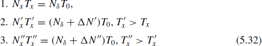
The measurement (conversion) of frequency and its deviations from the program-specified values is executed automatically during one time step T_q. Modes of one-time, cyclic or continuous measurements with high accuracy and speed are possible. The measurements are realized by the separate count of the impulse with the normalized width of two sequences with the frequencies f₀ and f_x, summation and the continuous comparison of the stored numbers with the specified number N_δ for determination of the moment of equality to one of them. Simultaneously, the quantization window T_q is formed, equal to the integer number of the periods τ of the lower frequency f (f_x or f₀). This interval is quantized by duration of the periods T of the greater frequency (f₀ or f_x). The accumulation of the number N in the frequency F counter is necessary, but it is an insufficient condition for the count termination and summation of periods of both sequences. The impulse count is stopped only at the moment of appearance of the wavefront of the consequent period, ensuring the multiplicity of T_q to duration of the period τ. After reading the numbers n = N_x and N, fixed in the counters of lower f and greater F frequencies accordingly, the measuring conversion is supplemented by the numerical according to the formulas:

where N = N_δ + ΔN is the total number of periods T, that was accumulated in the counter of the frequency F during the quantization window T_q; ΔN is the complement number to the specified number N_δ of the periods T that will be accumulated in the counter of the frequency F after its nulling up to the measuring termination.

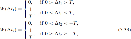
The time diagram of the count of the periods τ of the lower frequency f and the periods T of the greater frequency at the frequency measurement f is shown in Figure 5.8. It is obvious that:

where Δ_q = Δt₁ − Δt₂ is the absolute quantization error (the error of the method) of the time interval T_q. This error arises because of the non-synchronization of the first and last impulse of the frequency F with wavefronts of impulses of the frequency f, determining the start and the end of the quantization window.

The time of the measurement (conversion) is:

with the error, not exceeding the ±T. This time does not depend on the measurand frequency in the frequency range D₁. The range D₁ can vary from infralow frequencies up to the frequency f₀ = f_max. The latter is determined by the greatest possible frequency that can be counted by the timer/counter.

In case, when τ = T_x (mode f₀ ≥ f_x) and T = T₀ = 1 /f₀, Equations (5.15) and (5.17) should be written as:

If τ = T₀ and T = T_x (mode f_x > f₀), then:

The frequency range is extended up to 2D₁ and overlapped only by one specified measuring (working) range.

5.7.2 Methods of conversion for relative values

Unlike the algorithm for measurement of absolute values, the algorithm for measurement of relative values is executed in two steps [122]. The measurement of the ratio fx₁/fx₂ is executed without using the reference frequency f₀ (Figure 5.9).

The first step is used for the determination of the greater one of the two unknown frequencies. To this effect the following procedures are carried out:

Figure 5.9 Time diagram of method for frequency ratio measurements

1. The calculation of the number N₁ = 1/δ₁ according to the program-specified relative error of determination of the greater frequency.
2. The separate count.
3. The summation of T_x1 = 1/f_x1 and T_x2 = 1/f_x2 periods of impulse sequence.
4. The comparison of the obtained sums up to reaching the equality to the number N₁.

The impulse count of both frequencies is completed at the moment of accomplishment of this equality. The information about the greater of two frequencies is entered into the microcontroller.

The second step is used for measurement of the frequencies ratio f_x1/f_x2, if f_x1 ≤ f_x2, or f_x2/f_x1, if f_x1 ≥ f_x2. Thus:

1. The number N_δ = 1/δ is calculated on the program-specified relative error δ of ratio measurement.
2. The impulses of both sequences are calculated.
3. Each of the accumulated sums is compared period by period with the number N_δ according to the algorithm of the absolute method of the dependent count.

The integer number n of the periods τ is fixed into the counter of the lower frequency f (f_x1 or f_x2). The count of impulses of the frequencies f_x1 and f_x2 is stopped after the counting by the counter of the frequency F (fx₂ or f_x1) the number (N_δ; + ΔN) of the periods T. The result of measurement is calculated according to the formula:

and displayed in the specific units of measurement (relative, %, per mille ‰, etc.). With regard for the result of determination of the greater of the two frequencies, the calculations will be carried out according to the formulas:

Thus, the relative error of measurement of the frequency ratio will not exceed the program-specified error δ.

Let us consider another method for frequency ratio. The second method is more complex. Its realization requires the addition generator of the reference frequency f₀, the third counter of impulses for the frequency f₀ and more complex software for the microcontroller.

Due to exception of the procedure for determination of the greater frequency (Figure 5.9), the ratio f/F is measured by one step. The measurements of frequencies f and F are executed simultaneously according to the method of the dependent count for absolute values, but with some features. In this case, the following procedures are executed:

• The separate and simultaneous count of normalized impulses of frequencies F, f and f₀.
• Forming of the reference time intervals T_q1 and T_q2 equal to the sum of the integer of periods T and τ.
• Their simultaneous and independent quantization by duration of the period T₀.

The number of the latter is accumulated and continuously compared with the beforehand given N_δ = 1/δ. The accumulation of the number N_δ in the counter of the frequency f₀ is necessary, but there is the insufficient condition for the count termination and summation of the durations of periods τ and T. The impulse count of the greater frequency F is terminated at first at the moment of appearance of the impulse followed by its period T. Due to this the equation T_q1 = N_x1T is true. Simultaneously the result of the frequency F to code conversion (the numbers N_x1 and ΔN₁) is read out. Then the impulse count of the lesser frequency f is stopped. It happens at the moment of appearance of the impulse followed by its period τ. The last fact ensures the equality T_q2 = N_x2. After that the count of periods T₀ with simultaneous reading of the numbers N_x2 and ΔN₂, and determination of the greater of two frequencies f_x1 or f_x2 is stopped. The analog-to-digital conversion is supplemented by the calculations:

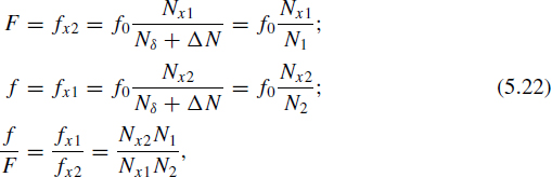
where ΔN₁ and ΔN₂ are the complementary numbers up to the number N_δ. They are read out from the counter of the reference frequency f₀ after the first and second interrupt. The ratio of periods T_x1 and T_x2 can be determined from Equations (5.22). Besides it is possible to determine the absolute and relative differences of two frequencies or periods; absolute and relative deviations of the value of controlled parameters from one or several program-specified values.

The circuitry of the first and second methods for frequency ratio conversion is rather simple. It does not require a lot of hardware and accepts their margin and the program choice of one of them. The example of such a universal converter for the ratio of two frequencies constructed with the most complex hardware is shown in Figure 5.10.

The microcontroller expands the possibilities of such converters and realizes the functions of transmission of the results of conversion of frequency deviation by the pulse-width or code-impulse signals. It is necessary for realization of digital intelligent distributed sensor systems, the multichannel converter, etc. The hardware–software realization of the method for frequency ratios expands the range of measurand frequencies, due to the use of the hardware and virtual counters, realized inside the microcontroller. Therefore, the range of measurand frequencies practically is unlimited even at low frequencies.

Figure 5.10 Frequency ratio f_x1/f_x2 to code converter

The realization of wide-range frequency converters requires two addition hardware counter dividers of input frequency, some triggers and digital logical circuits.

For both methods of measurement the time of quantization T_q is non-redundant in all ranges of measurand frequencies and can be varied in the limits:

The absolute error of the methods is:

The relative quantization error:

5.7.3 Methods of conversion for frequency deviation

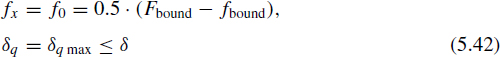
In some cases there is a necessity to convert deviations of frequency from the preset value into the code without additional hardware and with high software controlled accuracy or speed. The method of the dependent count allows these possibilities. Such a conversion assumes some arithmetic operations and is determined by the equation

where a, b and c are the certain constants, set in the same format and units of measurements, as the measuring results.

Thus, the following formulas are valid for numerical algorithmic transformations with the aim to determine the deviation of the measured frequency f_x with software-controlled accuracy or speed from one (as at the limiting control)

or some preset values (as at the admissible control)

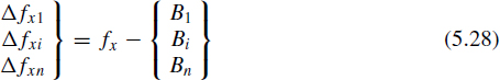
and frequency deviations

Let's specify, that the task of the control for frequency-time parameters of signals can also be solved: at the limiting control it will be determined if f_x <> f_xbasis, and at the admissible control, whether there is a controllable frequency inside some specified area of allowable values.

5.7.4 Universal method of dependent count

The algorithm of the universal method of the dependent count integrates algorithms of both absolute and relative methods. The distinctive feature of the measurement for absolute values according to the algorithm of the universal method of the dependent count is, that it will be executed in two steps. Owing to these, no additional measures for determination of the greater of two frequencies are necessary.

Thus, all three algorithms of the method include: the procedure of automatic count number of normalized on duration impulses, for assurance of the inequality τ T_{x min}; the procedure of period-by-period comparison of the accumulated sums with the specified number; the procedure of processing of results of measurements. Theoretically, the count does not bring in an error by the usage of appropriate devices for its implementation.

The comparison error that is determined by the speed of the used devices and a number of bits of compared numbers can be also neglected. The calculation error of the result of measurement under the specified formulas can be neglected as well. The rounding error is distributed according to the uniform unbiased (equiprobable) distribution law. Therefore, the error of the frequency-to-code conversion will be determined only by the quantization error, the reference frequency stability and the trigger error in case of a harmonic signal and the effect of interference.

The consequent digital signal processing: scaling, determination of the difference and deviation of measurand values from program-specified, minimax, statistical and weight signal processing, sensor characteristics linearization, extrapolations, etc. can be used for the further processing of the result of the measurement.

5.7.5 Example of realization

The simplicity of the method realization using minimum hardware is an important advantage. The schematic diagram of the frequency-to-code converter based on the universal method of the dependent count is shown in Figure 5.11.

At the beginning the measuring mode (absolute or relative values) and the required relative errors δ₁ and δ are set. Then the microcontroller calculates the numbers N₁, N_δ and initializes the counters CT1, CT2. The measurements begin after actuation of the trigger T4 by a start impulse through the logical element OR_1. Then the elements AND_5, AND_6 are actuated. The formed impulses with the frequencies f_x1 and f_x2 at ratio measurement or f_x1 and f₀ at frequency measurement (the trigger T3 is switched off) feed on the inputs of the decrement counters. The signal from the zeroized counter is fed on the interrupt input of the microcontroller. The microcontroller switches off the trigger T4 and terminates the impulse count of both frequencies.

If the frequency f_x2 was greater at the ratio measurement (the trigger T3 is actuated), the microcontroller downloaded the number N_δ = 1/δ only in the counter CT2 at repeated initialization. Then the trigger T1 is actuated again. The first impulse of the frequency f_x1 through the open element AND_1 and the element OR_1 actuates the trigger T4 again and switches off the trigger T1. The new count cycle of periods and the decrement of the counters begins: CT1 from the N_max = 2ⁱ (where i = 16, 32, 64); CT2 from the N_δ. After zeroizing the last one, the signal from the inverse output CT2 goes on the microcontroller's input. The μK actuates the trigger T1 again. The consequent impulse of the frequency f_x1 switches off the triggers T1, T4 and eliminates the count of impulses of both frequencies. The signal from the inverse output of T4 goes on the third microcontroller's input and eliminates the count at the ratio measurement f_x1/f_x2.

If f_x1 is the greater frequency, the microcontroller downloads the number N_δ only in the counter CT1 at initialization. The decrement of the counters is executed in a similar way from the values N_δ and N_max. Thus, the quantization window is formed. It is equal to the integer number of the periods T_x2 = 1/f_x2. After the last nulling, the signal from the inverse output of the trigger T4 goes again on the μK's input and eliminates the measurement. The μK reads the numbers N_x2 and ΔN₁ (or N_x1 and ΔN₂, if f_x1 ≤ f_x2) and calculates the result of the measurement according to Equation (5.21).

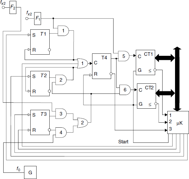
Figure 5.11 Schematic diagram of universal method of dependent count

The average value of frequency is measured similarly. The mode of determination of the greater frequency is also necessary in this case. Due to this, after completion of the second step of measurement with accounting the result on the first step, the μK calculates the result as:

The determination of the greater frequency is possible without necessity of execution of the first step. It requires some more complicated software.

Let's note that this scheme is one of the most complex hardware realizations of the method, except the multichannel synchronous one with the simultaneous conversion of frequencies in all channels. It can be realized in the silicon, PLD or FPGA. The most simple is the program-oriented realization [123–124]. The combine implementation [125] is somewhat more complex. In these cases, the measuring channel will be realized completely or partially on the virtual level inside the functional-logical architecture of the computer power.

5.7.6 Metrological characteristics and capabilities

The accuracy and time of measurement are the main characteristics of various methods for frequency-to-code conversion. These characteristics are the main quality indexes at any automatic measurements. However, in the case of frequency measurements they are more interconnected. The method of the dependent count differs from other conventional methods in that the indicated correlation is very loosed, because the quantization window T_q is non-redundant and, as it follows from Equation (5.16), practically does not depend on the measurand frequency. Moreover, the method of the dependent count has some additional possibilities. It is necessary to give them a quantitative evaluation.

5.7.7 Absolute quantization error Δ_q

Let's consider the time diagrams (Figure 5.12) illustrating one cycle of measurements of unknown frequencies with the periods τ₁, τ₂ > τ₁ and τ₃ > τ₂.

Figure 5.12 Time diagram of conversion cycle

Each next conversion begins at once after the initialization of the counters by the microcontroller. The number N_δ = 1/δ is written into the counter of the greater frequency F = 1/T. Both logical elements are opened and after arrival of the impulse of the lower frequency f₂ = 1/τ₂ the quantization window T_q will be formed. Impulses of the frequency f₂ with the duration t τ_min and impulses of the frequency F after the time 0 ≤ Δt₁ ≤ T are calculated in parallel. Therefore the numbers in the counters begin to decrement from 2¹⁶ in the counter of the lower frequency and from N_δ = 1/δ in the counter of the greater frequency.

If zeroing happens before the arrival of an impulse of the frequency F₂ (case 2), the impulse count proceeds and the counter decrement begins again from the number N_δ. Through the time interval (T − Δt′₂) after arrival of the last impulse of the ΔN′ the impulse of the lower frequency comes. It finishes the creation of the quantization window and eliminates the impulse count by both counters. The calculation (Equations (5.18) or (5.19)) begins after reading the numbers Nx′ and ΔN′ (the number N_δ is stored in μK's memory). The measurements in the first and the third cases are executed similarly. Thus, with the absolute quantization error Δ_q = Δt₁ − Δt₂, that does not exceed the |T | for all three cases (Figure 5.12) the following equations are true:

Let's note that the conversion of the unknown frequency f according to the method of the dependent count can be considered as the determination of the average frequency of the sequence consisting of the (N_δ + ΔN) impulses with the period T with the help of the rectangular weighting function of the single-level integrating window of Dirichlet. The duration of the window is equal to the integer number of periods τ. The Δt₁ and Δt₂ are independent random components of the quantization error Δ_q, because of non-synchronization of the Dirichlet window with the first and last impulse of the sequence with the period T. These components of errors are distributed according to the uniform, asymmetric distribution law:

with the expectation value |0.5T | and the variance D = T²/12.

The absolute error Δ_q is equal to the sum of components Δt₁ and Δt₂. It is distributed according to the symmetrical triangular distribution Simpson law with the following numerical characteristics:

• the expectation value M(Δ_q) = M(Δt₁) − M(Δt₂) = 0
• the maximum value Δ_{q max} = ±T
• the mean square error

  

• the variance D(Δ_q) = σ²(Δ_q) = T ²/6.

5.7.8 Relative quantization error δ_q

The relative quantization error δ_q characterizes more completely the accuracy of the measurement than the absolute one. It is obvious (Figures 5.8, 5.12) that the error arises because the variable time interval formed during the measurement is equal to the quantization window T_q = N_xτ = N_x/f. The interval T_q will be varied at the change of the frequency f. Therefore, the number N of the periods T (Figure 5.12) will also vary within the limits of 0–N_max due to the ΔN changes. The latter is determined by the duration of the time interval τ and the frequency F:

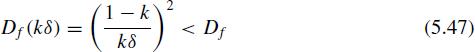
The error Δ_q is distributed according to the symmetrical distribution Simpson law. This error is maximal at the N = N_min = N_δ = 1/δ and minimal at the N = N_max = N_δ + ΔN_max = 2N_δ − 1. It is determined as:

where T_δ = T/δ is the program-specified time of measurement in the mode of the specified speed in addition to the mode with the specified accuracy δ. It is obvious

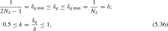
where k is the coefficient of the change of the error.

The dependencies of the error δ_q(δ, f_x) illustrating these features and advantages of the method are shown in Figure 5.13.

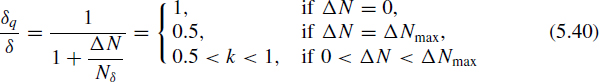
Thus, the equation T_q = nτ = N_x T_x is true for all the frequencies of the measuring range D₁. Each time, when it is defaulted, the specified number of the impulses N_δ is automatically increased on the ΔN due to the extension of the integrating Dirichlet window up to assurance of the multiplicity T_q and τ(T_x or T₀). Therefore, until N_δ ΔN the error Δ_q is constant, does not exceed the specified δ and identical at frequencies f_x < f₀ and f_x > f₀, symmetrical concerning the middle of D_f, in which f_x = f₀. The dependence of the error δ_q from the frequency begins to be apparent at increase of the number ΔN. The δ_q decreases on the f_bound and F_bound boundaries of the range D_f and becomes equal to 0.5δ. The error δ_q continues to decrease in relation to the 1/2N at further increase of the number ΔN, if the counter capacity allows.

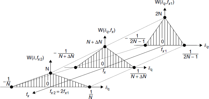
Figure 5.13 Distribution laws of the relative quantization error δ_q

Therefore, due to the method of the dependent count it is possible to realize the self-adopted mode of frequency measurements with the specified relative error δ or the time of measurement T in a broad range of frequencies from infralow up to high, limited by double value of the reference frequency f₀. Thus, the possibility of the extension of the range D_f in the lowest frequencies is determined only by the counter capacity m:

In hardware realization the decrease of the lower boundary f_bound can be reached due to increase of the used number of counters with the capacity m = 32, 48, 64 bits and are more, moreover by decrease of the frequency f₀. For combined and program-oriented realizations, the extension to low and infralow frequencies practically is not limited. It is only determined by the maximum acceptable time T_q = T_{x max} (Nx = 1). The high boundary F_bound is determined only by the greatest possible frequency of count for timers/counters and frequency dividers. Thus, the width of the frequency range in the common case is equal to:

5.7.9 Dynamic range

Let's determine the dynamic range of the frequency-to-code converter based on the hardware realization of the method of the dependent count. The decrement counters, used for its realization, limit the width of the range D_f. The high bound F_bound is determined by the maximum acceptable frequency f_clc, which can be calculated by these counters, and the low f_bound by the number of 16-bit counters. Therefore

Table 5.1 Dynamic range at Δδ_q = 0.5δ

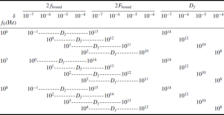
With regard for the above, the decrease of the error δ_q relative to the specified δ does not exceed the values:

Having accepted for simplification ΔN_max ≈ τF, N_x = 1, and N ≈ 2N_δ, we receive the formulas for determination f_bound, F_bound and D_f:

The calculated results according to the Equation (5.41) for that case, when Δδ_q = 0.5 δ, are adduced in Table 5.1. The width of the frequency range D_f is shown in Table 5.2.

The possibilities of the symmetrical extension and shifting of the range D_f by the decrease of the error δ and the change of the frequency f₀ are obvious from these tables. By the decrease of the error δ the range D_f symmetrically extends concerning the middle–the frequency f₀, for which:

The time T_q is minimum possible:

Table 5.2 The width of the frequency range D_f

In frequency counters based on traditional methods of measurement, the relative quantization error δ_q increases according to the hyperbolic law by the decrease of the measurand frequency f_x or the period T_x:

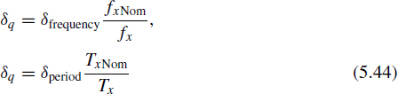
Therefore, their range D_f is much narrower. It is asymmetric concerning the frequency f₀ and equals only to one decade. Thus δ_q = 10δ_frequency and δ_q = 10δ_period at f_x = 0.1 f_xNom T_x = 0.1T_xNom. Unlike the method of the dependent count the quantization window T_q and the quantization frequency f_q remain constant within the limits of one decade:

They are redundant for all measurand frequencies and periods from the range D_f, except the nominal one. Further increase of the range D_f is possible. However, it requires additional hardware and special technical solutions.

The method of the dependent count allows to set not only the maximum error δ, that does not depend on the measurand frequency, but also the coefficient k > 0.5 (for example, k = 0.9–0.98 or lower). This coefficient can be used for limitation from below the error δ_q (in the boundaries kδ < δ_q < δ) and from above the time T_q. However, the range D_f (kδ) is narrowed down. In this case, Equations (5.41) should be rewritten:

The ways of the extension of the range D_f(kδ) or its shifting remain similar to those explained above. The δ decreasing does not require additional hardware.

5.7.10 Accuracy of frequency-to-code converters based on MDC

The accuracy of conversion and metrological reliability are the most important performances of a smart sensor. The main components of static and dynamic errors of the method of the dependent count are shown in Figure 5.14.

The static error is stipulated by the trigger error, the reference frequency instability, the quantization error and the calculating error. The latter is determined by calculation of the result of measurement according to the specified formulas with the use of the numbers N_x, ΔN and consequent rounding of the result.

Figure 5.14 Components of static and dynamic errors

The dynamic error is stipulated by the change of the measurand frequency during the time interval T_q and between the cycles of measurement. The method of the dependent count organizes the two-channel mode of continuous frequency measurement without loss of speed and accuracy. In this case, the dynamic error will be determined only by duration of the quantization window T_q.

The maximal δ_{f max} and the mean-square static errors σ_f are determined as:

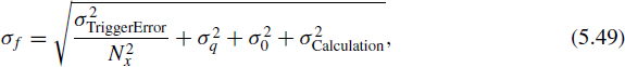
where δ_{TriggerErrormax} and σ_TriggerError, δ_{q max} and σ_q, δ_{0 max} and σ₀, δ_Calculation and σ_Calculation are the maximal relative and the mean-square trigger error, the quantization error, the reference frequency error and the calculation error, respectively.

At first, let us consider the components of the static error.

5.7.11 Calculation error

The use of modern μP and μK realizes the condition rather easily:

5.7.12 Quantization error (error of method)

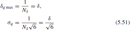
It is determined by the program-specified error δ and does not depend on the measurand frequency. It is supposed, that the counters do not bring in the additional component to this error because of the time and temperature trigger instability.

5.7.13 Reference frequency error

The reference clock quartz generator (with the period T₀ and the duration τ T₀ (Figure 5.12) is a source of the error δ₀. Its influence on the result follows from the definition of the measurand frequency according to the method of the dependent count (Equations (5.18) and (5.19)). It is stipulated by the long-term and short-term frequency instability:

The change of the frequency f₀ at the constant measurand frequency f_x will result in changing of the number N, and consequently, of the result. In the mode, when f_x > 0, the time interval T_q will be varied. Thereof the result of measurement will be also changed.

The long-term changes depend on the systematic deviations of the frequency f₀ stipulated by the time drift. It is 10⁻⁹–10⁻¹¹ for one day, and causes the systematic component of the error δ₀.

The short-term changes depend on the frequency fluctuation. They cause the random component of the error δ₀ because of short-term temperature and time drifts.

The systematic component of the error δ₀ can be reduced by the correction of the frequency error up to the random level. In practice it is necessary to take into account only temperature and time instabilities, that is equal to ≈10⁻⁷–10⁻⁹ and is determined by the quality factor of a quartz resonator. The last one can achieve the value 50 × 10⁻⁶ and higher for precision quartz resonators. Due to this the random variation of the frequency of the reference generator can be not worse than 10⁻¹¹.

Therefore, the error δ₀ should be considered as a random error with the uniform distribution law within the boundaries ±δ_{0 max}:

The temperature control and temperature compensator for quartz generators reduce the error δ_{0 max} and increase considerably the frequency stability.

The use of external generators with more stable reference frequency, connected with the atomic frequency standard is rather perspective. The caesium and rubidium frequency standards are widely used in this case. Their instability does not exceed (2–3) × 10⁻¹² and (1–3) × 10⁻¹¹ accordingly. For example, the use of the device OFS2/2 from Gould Advance Corporation guarantees the frequency stability not worse than ±1 × 10⁻¹⁰ during 1000 seconds. It determines the maximal value of the period T_x = T_q, which can be measured with such stability.

As the relative error δ can be varied over a wide range, each time, when δ > δ_{0 max} in 3–5 times it is possible to consider the latter very little and not take into account Equations (5.48) and (5.49).

5.7.14 Trigger error

The input blocks F1 and F2 (Figure 5.11), consist of an attenuator, a controlled amplifier and a Schmitt trigger. They select the period of the input signal and form the sequence of rectangular impulses with the period T′_x and the duration t T _x ′_min, and ensure the triangular unbiased distribution law of the quantization error δ_q. Because of incomplete signal processing limited by possibilities of the F1 and F2, the period T′_x differs from the real period T_x of the frequency f_x on the value ±ΔT_x = ±δ_TriggerError T_x. The quantization window T′ _q = N′_xT_x′ will differ from the conventional true value T_q on the value ±N′ _xΔT_x′ which can be large. Therefore, the accuracy of the frequency-to-code converter can be determined by the error δ_{TriggerErrormax}, instead of the errors δ_{0 max} and δ_{q max}. Especially it is characteristic for conversion of low frequencies of the harmonic signal (N_x → 1).

The first of two components of the is the trigger level setting error due to deviation of the actual trigger level from the set trigger level. The second component of the error δ_{TriggerErrormax} occurs when the measurement starts or stops too early or too late because of noise on the input signal. At rather low noise level the influence on the selection of the period T_x can be reduced and even eliminated by a choice of the trigger hysteresis. The smooth narrow-band noise changes the moment of operation of the input device and can also reduce to greater difference of the duration T_x′ from the T_x. In all cases, the noise appears both at the beginning and at the end of each period of the input signal. By the broadband noise, it is difficult to determine the period T_x, as the time intervals between adjacent operations of the input device do not characterize the period T_x any longer. Special measures, for example, the usage of input filters with the cut-off frequency are necessary for the elimination of this influence:

Thus, fluctuations of the operation level and noise reduce work of the trigger up to or after the necessary moment. Therefore because of such a false operation of the Schmitt trigger, the time interval T_q′ = T_q ± N′_xΔtx′ will be quantized by impulses with the period T₀ if f_x ≤ f₀ or T_q = N_xT₀ by impulses with the period T′_x = T_x± ΔT_x, if f_x > f₀ instead of the interval T_q = N_xT_x. If special measures are not employed, there will be an absolute error of measurement of the frequency Δf′_x.

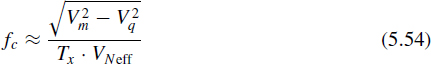
The mean-square value of the deviation ΔT_x of the period T_x of a harmonic signal and the relative error of definition of its conventional true value are determined as in [95]:

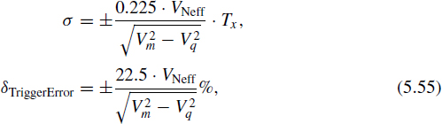
where V_Neff is the effective noise voltage; V_m is the amplitude of the sinusoidal voltage of the measurand frequency.

Even the low noise reduces in significant errors . So, for example, if V_m = 10 V, V_Neff = 0.1 V (1% in relation to the input signal) and the quantization level V_q = 0.3 V, the error will be ≈ ±0.225%. As it was determined at a signal/noise ratio equal to 40 dB the error will be = 0.3%.

With the aim of decreasing the it is necessary to quantize some periods . In this case, the error will be decreased N_x times. In the case when higher frequencies are measured and N_x 1, the error can be neglected.

By the measurement of the frequency of impulse sequence, the error will decrease. In this case, it depends on the number N_x, the period T_x, the set trigger level, its drift Δ and the wavefront steepness S [95]:

The error can also be neglected by measuring frequency f_x of pulses with steep wavefronts.

Now let us consider the dynamic error and its components. By frequency measurements, this error essentially depends on the dynamic properties of the researched process and the speed of the method of measurement. The decrease of the dynamic error is possible by the increase of speed and continuous correction of the measurement results.

The method of the dependent count has the highest speed at measurement of all frequencies of the range D_f and consequently allows reduction of the dynamic error for the same frequencies of researched physical values, as well as for traditional methods of measurement. The main components of the dynamic error are the tracking error and the approximating error.

The first component depends on the time T_q. The result of the measurement of duration of the period or several periods of low frequencies composing the time T_q, corresponds to their average value on the time interval equal to their duration. The inevitable availability of such an average and also the change of the researched value during the latency time if it is not eliminated, is the reason of the rise of the so-called average error.

The second component is the approximation error of the continuously varying value of the lattice function with the appropriate approximation between points of its discrete values. The approximation error is determined by the digitization interval and a kind of approximation. In one-channel and multichannel measuring instruments the digitization interval cannot be lower than the time of the measurement T_q.

The decrease of the dynamic error can be reached by minimization of the time T_q by the choice of the algorithms, the eliminating latency time of the next cycle of conversion.

The dynamic error should not exceed the static. Under this condition, the acceptable time T_q at the known frequency of change of the researched value and its maximum value at the selected T_q are determined. This algorithm can also be used at higher frequencies of the range D_f, if the time of the measurement is large, even in the case of the method of the dependent count.

5.7.15 Simulation results

The quantization error δ_q is the function of many variables and is determined by the given relative error δ and the frequencies f and F. This function δ_q(δ, F, f) is piecewise-smooth and has a final number of discontinuities of the first kind. In this analysis of the family of characteristics we will start from the function δ_q(δ, F) at f = const. All characteristics of the given family are symmetric concerning the middle of the range D_f(δ_i, F). In this point ΔN = 0 and f = F. Therefore in these points and their neighbourhoods δ_q = δ_{q max} = δ. Change of the ordinate δ_i for any of these functions at F = const reduces in its parallel moving up (down) at increase (decrease) of the error δ_i. By this, the range D_f, within the limits of which the condition (5.36) is satisfied varies. If the counter capacity is sufficient, the frequency measurement outside the range D_f with the errors δ_q < 0.5 δ is possible. Simultaneously the number N_break of discontinuity of the first kind will be varied. By this, their number is increased with decrease of the error δ.

The change of the frequency F at δ = const reduces the shift of the characteristic of the family towards low frequencies, at its decrease, and towards high ones, at its increase, without the change of the range D_f. However, the maximum measurand frequency f_max ≤ 2F therefore will be varied.

Now let's consider the characteristic δ_q(f, F) at δ = const. If the frequency f varies relatively to the F, the dependence of the error δ_q from the frequency f becomes apparent in a various degree from some value. Due to the self-adopting of the method this dependence is expressed much more poorly than in the traditional methods of comparison. The number ΔN is increased from 1 up to ΔN_max symmetric relatively to the frequency F = f₀ boundaries f_bound and F_bound of the range D_f because of the automatic change of the Dirichlet window. The error δ_q is decreased from δ up to the minimal value δ_{q min} = 0.5δ. In the common case, on the boundaries D_f:

Let us investigate the required frequency dependence of the error δ_q, its jumps in the points N_break, the boundaries of the discrete steps and their value Δδ_q in more detail. For simplification we shall consider only the first half of the D₁ of the range D_f of the function δ_q(f, F), in which f = f_x ≤ F₀ = F and δ = const and f₀ = const. Due to the symmetry, the obtained results will also be true for the second half of the D₂ of the range D_f.

The mathematical analysis of the function δ_q(f_x, f₀) on continuity has confirmed the availability of discontinuities of the first kind and has shown, that by the change of the frequency f_x in the last interval (N_x − 1)T_x … N_xT_x in the quantization window T_q the change of the number N is a reason for jumps in the points N_break. It makes the following conclusions.

(1) The values of the jumps Δδ_qi, the number ΔN_i = t′_if₀ and the time intervals 0 ≤ t′ ≤ T_x are decreased and tend to zero by the increase of the frequency f_x. Therefore in this greater part of both halves of the range D_f contiguous to its middle, the plot of the function δ_q(f_x, f₀) presents a significant number of slanting sites of hyperbola of various lengths, divided by the jumps Δδ_qi in the points N_break with co-ordinates:

In accordance with the decrease of the number ΔN_i the value of the jumps Δδ_qi decreases, and the segments of the hyperbolas δ_q(f_x, f₀) juxtapose up to full junctions and coincide with the plot of a hypothetical (ideal) method. The latter represents a direct line, parallel to the axis of frequencies with the ordinate δ. Therefore the error δ_q practically does not depend on the frequency f_x (Figure 5.15(a). Such a dependence is saved by the change of the frequency f₀ over the wide range and the error δ = 0.0005–0.00005.

(2) By the decrease of the frequency f_x the Dirichlet window is extended. The duration t′_i, the number ΔN_i and Δδ_qi between adjacent partial segments of hyperbolas composing the function δ_q(f_x, f₀) is increased. On the low bound f_bound the number ΔN = ΔN_max = N_δ − 1, the error δ_q = δ_{q min} = 0.5δ, and Δδ_q = 0.5δ.

The simulation results of the functions δ_q(f_x, f₀) for a wide range of low frequencies are shown in Figure 5.15(b). The segment of the piecewise-smooth function composed from the partial segments of the hyperbolas at f₀ = 20 kHz and f_x 1–8 Hz is shown in the foreground of the figure. The analysis of these functions for other values of f₀ has confirmed the dependence of the error δ_q from the f_x in the extreme minority of the range D₁ that exists and weakens by the increase of the f₀.

Thus, in both cases the error δ_qi never exceeds the given value δ_i in the whole range D_f of measurand frequencies from f_bound up to F_bound. Each function from the set δ_qi(f_x, f₀) at δ_i = const is piecewise-smooth. It consists of the final number of partial segments of hyperbola divided by jumps of the various value δΔ_qi in the discontinuities N_break of the kind. Their number considerably increases by the decrease of the program-specified error δ.

Let's determine the boundaries of discontinuities of the piecewise-smooth function δ_q(δ, f_x) and the value of the jumps Δδ_q in the points N_break between them. For that purpose, we shall take the advantage of a known technique and Equation (5.58). By the increase of the frequency f_x and approximation to the point N_break from the left the error δ_q goes to the limit:

Figure 5.15 Simulation results: (a) the dependence of the quantization error on the frequency in the whole range of measurand frequencies; (b) the dependence of the quantization error on frequency in the low frequency range; (c) the dependence of time of measurement on frequency and error of measurement

and the left-side boundary of the function will be formed.

By the decrease of the frequency f_x and approximation to the point N_break from the right the error δ_q goes to the limit:

and the right-side boundary of the function will be formed.

As δ_q(N_break–0) ≠ δ_q(N_break + 0), the function has the discontinuity in the point N_break and the finite jump Δδ_q, determined as:

The negative sign specifies that the left boundary is always more than the right one and by the decrease of the frequency f_x the error δ_q decreases and the jump Δδ_q increases. By this, the time T_q is increased at the cost of the extension of the Dirichlet window. As follows from Equations (5.17) and (5.18), the Dirichlet window practically does not depend on the measurand frequency. It is variable and non-redundant for each of the frequencies from the range D₁ and is set up automatically during the measurement. Therefore, in comparison to all known methods, the method of the dependent count is a self-adopted method. Due to this, the method has high metrological performances. The real function δ_q(f_x, f₀) coincides in greater part of the range with ideal, hypothetical. The simulation results of the set of the functions t_x(δ, f_x) at f₀ = const are shown in Figure 5.15. They confirm high dynamic properties of the method, due to which the dynamic error of the measurement is minimal possible.

5.7.16 Examples

In order to compare the method of the dependent count with the standard counting methods as well as with other advanced methods for the frequency-to-code conversion let us determine the coefficient of variation for the quantization error α = δ_{q max} /δ_{q min} for these methods. So, for the method of the dependent count if f_x is lower of two frequencies (f_x = f), and f₀ is greater of the frequencies (f₀ = F), i.e. f_x < f₀, from the following equations

and taking into account Equation (5.34) we will have

or

At f_x > f₀

Let's determine how many times the quantization error will be varied by the measuring frequency f_x = 2 Hz, if f₀ = 10⁶ Hz and N_δ = 10⁶ (δ = 10⁻⁶ × 100% = 0.0001%). From Equation (5.64) we have

i.e. the greatest error δ_max = 1/N_δ = 10⁻⁶, and the lowest δ_min = 0.67 × 10⁻⁶. As the greatest quantization error for the method of the dependent count is constant for any measurand, it is possible to characterize the possible range of variation of this error in the specified measuring range of frequencies by the coefficient of variation α. From this example it follows that the error variation is not more than 1.5 times in the frequency range 2–10⁶ Hz (the time of the measurement is constant for the given quantization error). By the use of the standard direct counting method or the indirect method measuring period, the variation of the quantization error will be 500 000 (at the same time of measurement).

Let us consider another example. It is necessary to measure f_x = 10⁴ Hz at f₀ = 10⁶ Hz and N_δ = 10⁴. According to the method of the dependent count the maximum time of conversion (5.17) is

In turn, according to the standard counting method, the time of measurements necessary for the same accuracy is T_{q max} = 0.5 sec. In other words, the time of measurement for the proposed method is non-redundant in all specified measuring ranges of frequencies. In the standard counting method, the time of measurement is redundant, except for the nominal frequency. Moreover, for the method of the dependent count the time of measurement can be varied during measurements depending on the assigned error.

5.8 Method with Non-Redundant Reference Frequency

Power consumption and dissipation on the elements becomes actual by smart sensor creation. The dynamic average power of a circuit can be given as

where V_DD is the supply voltage; f_clc is the clock frequency; C_eff is the effective capacitance of the circuit [126]. V_DD and C_eff are constant for the specific integrated circuit and technology. For many smart sensors V_DD is reduced up to 2.8–3.5 V. The power consumption is directly proportional to the system clock. If the clock speed doubles, the current doubles. Obviously, power can be saved by operating the device at the lowest possible clock speed [127]. The reduction of f_clc is in contradiction to that necessary to increase the metrological performances for precise measurements. In the majority of methods for frequency-to-code conversion, the reference frequency f₀ directly influences the conversion accuracy: the reduction of f₀ will increase the quantization error. In order to eliminate this inconsistency, another self-adapting method of frequency-to-code conversion with non-redundant reference frequency f₀ was proposed [114].

The essence of this method consists of the following. The embedded microcontroller or the arithmetic unit calculates the value of the necessary reference frequency according to the given quantization error δ_i:

where k = 1/T₀ = const (T₀ is the first reference gate period). The reference frequency f_0i, which is received by division/multiplication of the clock frequency f_clc and the measurand frequency of a quartz generator is calculated by two counters. The time of measurement is equal to the integer number of periods of f_x. This frequency is calculated similarly, as for the majority of advanced methods for frequency-to-code conversion:

The quantization error does not exceed that given beforehand:

Similar to the other advanced methods for frequency-to-code conversion, this method ensures a constancy of the quantization error in the total specified measuring range of frequencies–from infralow up to high frequencies. Besides that, the reference frequency f_0i is non-redundant and determined by the given quantization error δ_i. Thus, by the use of the method with the non-redundant reference frequency in smart sensors it is possible to receive further benefits. It has a high accuracy of measurement, a constancy of the quantization error and a reduction of the power dissipation during the conversion by the use of the lower (on the average by 1–2 order) reference frequency.

Modern achievements in microelectronics easily realize this method with the minimum possible hardware. The MSP430 microcontroller family for metering applications from Texas Instruments [128] is the most appropriate for realization of such a method for frequency-to-code conversion. These microcontrollers have capabilities that make them suitable for low-power embedded applications. As follows from this reference, one of the main characteristics of a power-efficient microcontroller core is the flexible clocking. This performance makes the MSP430 microcontroller family ideally appropriate.

The system clock frequency f_system in the MSP430 microcontroller family depends on two values:

where N(3 − 127) is the multiplication factor; f_crystal is the frequency of the crystal (normally 32 768 Hz). The normal way to change the system clock frequency is to change the multiplication factor N. The system clock frequency control register SCFQCTL is loaded with (N − 1) to achieve the new frequency [129].

Figure 5.16 Connection of frequency-time domain signal to the MSP430

Figure 5.16 shows the connection of the frequency signal to the MSP430 microcontroller. It can be connected to any of the eight inputs of Port0 and counted via the interrupt. If the frequencies to be measured are above 30 kHz then the universal timer/port or the 8-bit interval timer/counter may also be used for counting. The first reference time window is formed by the basic timer.

If the information to be converted is represented by pulse distances or pulse widths then it is also easy to be converted with the MSP430. The left part of Figure 5.16 shows how to do this.

The signal to be converted is connected to one of eight inputs of Port0. Each one of these I/Os allows interrupt on the trailing and on the leading edge. With the basic timer an appropriate timing is selected for the required resolution and the conversion is made. The universal timer/port may be used for this purpose too: the pulse to be measured is connected to the pin CIN and the time measured from edge to edge.

Even better resolution is possible with the Timer_A. The input signal is connected to one of the TA-inputs and the capture register is used for the time measurements.

5.9 Comparison of Methods

For choice of method for frequency-to-code conversion, it is expedient to prefer one that has high metrological characteristics and simple realization by its universality. The main performances of all the methods considered above are adduced in Table 5.3. Here number 1 is the indirect counting method (period measurement); 2 is the standard direct counting method (frequency measurement); 3 is the ratiometric counting method; 4 is the reciprocal counting method; 5 is the M/T counting method; 6 is the constant elapsed time (CET) method; 7 is the single-buffered and double-buffered method; 8 is the DMA transfer method; 9 is the method with the non-redundant reference frequency; 10 is the method of the dependent count.

Table 5.3 Main performances of methods for frequency-to-code conversion

Figure 5.17 Width frequency ranges D_f for different methods of frequency-to-code conversion

As it can be seen from the table, the majority of modern advanced counting methods overcome the demerit inherent to classical conversion methods. Namely, it means the inconstancy of the quantization error in all specified ranges of converted frequencies. However, most of them (methods with the constant conversion time as well as with the slightly varied conversion time) have a redundant conversion time for all frequencies, except the nominal one. The exceptions are the method of the dependent count and the classical indirect counting method (period measurement). Only one of methods, namely the method of the dependent count measures the frequency f_x ≥ f₀, and only one method, namely method 9 has the non-redundant reference frequency.

Conversion ranges for all considered methods are shown in Figure 5.17.

5.10 Advanced Method for Phase-Shift-to-Code Conversion

The phase shift φ_x between two periodic sequences of pulses with the period T_x can be converted by the method of coincidence [104]. Time diagrams of the method are shown in Figure 5.18. In this case the number N₁ pulses with the period T₀ and the number N′₁ pulses of the first sequence T_x between coincident pulses of these sequences is counted. Then

Similarly, the number N₂ of pulses T₀ and the number N′₂ of the second sequence with the period T_x, shifted on the t_x and taking place between the first moment of coincidence of the first pair of pulses and the nearest moment of coincidence of the second pair of the pulse are counted. Then

From these two equations, we receive the formula for the phase-shift calculation

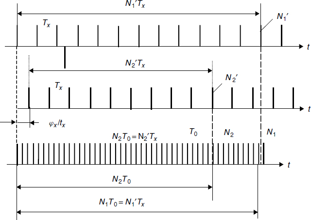
Figure 5.18 Time diagrams of the method of coincidence for phase-shift-to-code conversion

and for the converted time interval

The analysis of Equations (5.71) and (5.74) shows that φ_x and t_x do not depend on the period T_x. Conversion errors will be determined mainly by pulses duration only. For reduction of these errors, the method of forming of pulse packets of coincidences can be used. Thus, the absolute error of measurement for t_x can be reduced up to 0.5 × 10⁻¹² s and the absolute conversion error for the phase shift φ_x up to 0.05° at 1 MHz.

Summary

Due to advanced methods for frequency-to-code conversion, it is possible to achieve a constant quantization error for all ranges of converted frequencies.

The method of the dependent count is optimal for microcontroller-based frequency-to-code converters of a new generation for the measurement of absolute and relative frequencies in smart sensors. The developed conversion technologies based on the method of the dependent count open the possibilities of the creation of frequency-to-code converters of a new generation.

The accuracy of conversion is one of the most important quality factors for smart sensors that together with reliability characterize their serviceability and high metrological trustiness of obtained results. In traditional methods and frequency-to-code converters it predetermines such metrics of the economic efficiency as dimensions, the weight, the power consumption and the cost price. As a rule, cheaper converters have low accuracy and reliability. The method of the dependent count breaks this link and ensures higher metrics economic efficiency. Among them are:

• The self-adapting mode of measurement for frequency or a period, absolute and relative deviations and ratios. Due to this mode the error of conversion is constant for a wide range of measurand frequencies and the maximal quantization error does not depend on latter.
• Intellectualization of the measurements.
• Programmability of characteristics and functionalities at high metrological trustiness of the obtained results.
• The non-redundant conversion time for all frequencies of the measuring range: from infralow up to high frequencies. Due to this the time of quantization is a variable, set up individually during the quantization for each of frequencies according to the program-specified relative error and thereof is minimal possible.
• The possibility to measure various electrical and non-electrical values transformed beforehand into the frequency with representation of the results into program-specified units.
• The parallelism at synchronous measurements of frequencies practically without the degradation of metrological and dynamic characteristics.
• High efficiency of measurements by super accurate measurement by using an external frequency standard.
• The possibility of creating virtual measuring instruments and systems.

All these are possible due to the simple circuitry and the use of the computational power (microcontroller) as part of the measuring channel.

Due to the method of the dependent count precision and multifunctional smart sensor systems will be more available for customers for the execution of reference measurements at the level of accuracy and stability of the physical constants, as, for example, in the case of the proposed measuring instrument of the magnetic induction based on nuclear magnetic resonance [130].

The method of the dependent count (the method with the non-redundant conversion time) and the method with the non-redundant reference frequency are self-adapting. The first chooses automatically the required conversion time in order to provide the set value of the conversion error. The second method chooses automatically the reference frequency on the set value of the conversion error, thus saving the power consumption in those conditions of the measurement when a precise conversion is not required.