
Probabilistic Models for Classification
Hongbo Deng
Yahoo! Labs
Sunnyvale, CA
[email protected]
Yizhou Sun
College of Computer and Information Science
Northeastern University
Boston, MA
[email protected]
Yi Chang
Yahoo! Labs
Sunnyvale, CA
[email protected]
Jiawei Han
Department of Computer Science
University of Illinois at Urbana-Champaign
Urbana, IL
[email protected]
3.1 Introduction
In machine learning, classification is considered an instance of the supervised learning methods, i.e., inferring a function from labeled training data. The training data consist of a set of training examples, where each example is a pair consisting of an input object (typically a vector) x = 〈x1,x2, …,xd 〉 and a desired output value (typically a class label) y ∈{C1,C2, …,CK}. Given such a set of training data, the task of a classification algorithm is to analyze the training data and produce an inferred function, which can be used to classify new (so far unseen) examples by assigning a correct class label to each of them. An example would be assigning a given email into “spam” or “non-spam” classes.
A common subclass of classification is probabilistic classification, and in this chapter we will focus on some probabilistic classification methods. Probabilistic classification algorithms use statistical inference to find the best class for a given example. In addition to simply assigning the best class like other classification algorithms, probabilistic classification algorithms will output a corresponding probability of the example being a member of each of the possible classes. The class with the highest probability is normally then selected as the best class. In general, probabilistic classification algorithms has a few advantages over non-probabilistic classifiers: First, it can output a confidence value (i.e., probability) associated with its selected class label, and therefore it can abstain if its confidence of choosing any particular output is too low. Second, probabilistic classifiers can be more effectively incorporated into larger machine learning tasks, in a way that partially or completely avoids the problem of error propagation.
Within a probabilistic framework, the key point of probabilistic classification is to estimate the posterior class probability p(Ck|x). After obtaining the posterior probabilities, we use decision theory [5] to determine class membership for each new input x. Basically, there are two ways in which we can estimate the posterior probabilities.
In the first case, we focus on determining the class-conditional probabilities p(x|Ck) for each class Ck individually, and infer the prior class p(Ck) separately. Then using Bayes’ theorem, we can obtain the posterior class probabilities p(Ck|x). Equivalently, we can model the joint distribution p(x,Ck) directly and then normalize to obtain the posterior probabilities. As the class-conditional probabilities define the statistical process that generates the features we measure, these approaches that explicitly or implicitly model the distribution of inputs as well as outputs are known as generative models. If the observed data are truly sampled from the generative model, then fitting the parameters of the generative model to maximize the data likelihood is a common method. In this chapter, we will introduce two common examples of probabilistic generative models for classification: Naive Bayes classifier and Hidden Markov model.
Another class of models is to directly model the posterior probabilities p(Ck|x) by learning a discriminative function f (x) = p(Ck|x) that maps input x directly onto a class label Ck. This approach is often referred to as the discriminative model as all effort is placed on defining the overall discriminative function with the class-conditional probabilities in consideration. For instance, in the case of two-class problems, f (x)= p(Ck|x) might be continuous value between 0 and 1, such that f < 0.5 represents class C1 and f > 0.5 represents class C2. In this chapter, we will introduce several probabilistic discriminative models, including Logistic Regression, a type of generalized linear models [23], and Conditional Random Fields.
In this chapter, we introduce several fundamental models and algorithms for probabilistic classification, including the following:
- Naive Bayes Classifier. A Naive Bayes classifier is a simple probabilistic classifier based on applying Bayes’ theorem with strong (naive) independence assumptions. A good application of Naive Bayes classifier is document classification.
- Logistic Regression. Logistic regression is an approach for predicting the outcome of a categorial dependent variable based on one or more observed variables. The probabilities describing the possible outcomes are modeled as a function of the observed variables using a logistic function.
- Hidden Markov Model. A Hidden Markov model (HMM) is a simple case of dynamic Bayesian network, where the hidden states are forming a chain and only some possible value for each state can be observed. One goal of HMM is to infer the hidden states according to the observed values and their dependency relationships. A very important application of HMM is part-of-speech tagging in NLP.
- Conditional Random Fields. A Conditional Random Field (CRF) is a special case of Markov random field, but each state of node is conditional on some observed values. CRFs can be considered as a type of discriminative classifiers, as they do not model the distribution over observations. Name entity recognition in information extraction is one of CRF’s applications.
This chapter is organized as follows. In Section 3.2, we briefly review Bayes’ theorem and introduce Naive Bayes classifier, a successful generative probabilistic classification. In Section 3.3, we describe a popular discriminative probabilistic classification logistic regression. We therefore begin our discussion of probabilistic graphical models for classification in Section 3.4, presenting two popular probabilistic classification models, i.e., hidden Markov model and conditional random field. Finally, we give the summary in Section 3.5.
3.2 Naive Bayes Classification
The Naive Bayes classifier is based on the Bayes’ theorem, and is particularly suited when the dimensionality of the inputs is high. Despite its simplicity, the Naive Bayes classifier can often achieve comparable performance with some sophisticated classification methods, such as decision tree and selected neural network classifier. Naive Bayes classifiers have also exhibited high accuracy and speed when applied to large datasets. In this section, we will briefly review Bayes’ theorem, then give an overview of Naive Bayes classifier and its use in machine learning, especially document classification.
3.2.1 Bayes’ Theorem and Preliminary
A widely used framework for classification is provided by a simple theorem of probability [5, 11] known as Bayes’ theorem or Bayes’s rule. Before we introduce Bayes’ Theorem, let us first review two fundamental rules of probability theory in the following form:
p(X)=∑Yp(X,Y)(3.1)
p(X,Y)=p(Y|X)p(X).(3.2)
where the first equation is the sum rule, and the second equation is the product rule. Here p(X,Y) is a joint probability, the quantity p(Y|X) is a conditional probability, and the quantity p(X) is a marginal probability. These two simple rules form the basis for all of the probabilistic theory that we use throughout this chapter.
Based on the product rule, together with the symmetry property p(X, Y) = p(Y, X), it is easy to obtain the following Bayes’ theorem,
p(Y|X)=p(X|Y)p(Y)p(X),(3.3)
which plays a central role in machine learning, especially classification. Using the sum rule, the denominator in Bayes’ theorem can be expressed in terms of the quantities appearing in the numerator
p(X)=∑Yp(X|Y)p(Y).
The denominator in Bayes’ theorem can be regarded as being the normalization constant required to ensure that the sum of the conditional probability on the left-hand side of Equation (3.3) over all values of Y equals one.
Let us consider a simple example to better understand the basic concepts of probability theory and the Bayes’ theorem. Suppose we have two boxes, one red and one white, and in the red box we have two apples, four lemons, and six oranges, and in the white box we have three apples, six lemons, and one orange. Now suppose we randomly pick one of the boxes and from that box we randomly select an item, and have observed which sort of item it is. In the process, we replace the item in the box from which it came, and we could imagine repeating this process many times. Let us suppose that we pick the red box 40% of the time and we pick the white box 60% of the time, and that when we select an item from a box we are equally likely to select any of the items in the box.
Let us define random variable Y to denote the box we choose, then we have
p(Y=r)=4/10
and
p(Y=w)=6/10,
where p(Y = r) is the marginal probability that we choose the red box, and p(Y = w) is the marginal probability that we choose the white box.
Suppose that we pick a box at random, and then the probability of selecting an item is the fraction of that item given the selected box, which can be written as the following conditional probabilities
p(X=a|Y=r)=2/12(3.4)
p(X=l|Y=r)=4/12(3.5)
p(X=o|Y=r)=6/12(3.6)
p(X=a|Y=w)=3/10(3.7)
p(X=l|Y=w)=6/10(3.8)
p(X=o|Y=w)=1/10.(3.9)
Note that these probabilities are normalized so that
p(X=a|Y=r)+p(X=l|Y=r)+p(X=o|Y=r)=1
and
p(X=a|Y=w)+p(X=l|Y=w)+p(X=o|Y=w)=1.
Now suppose an item has been selected and it is an orange, and we would like to know which box it came from. This requires that we evaluate the probability distribution over boxes conditioned on the identity of the item, whereas the probabilities in Equation (3.4), (3.5), (3.6), (3.7), (3.8) and (3.9) illustrate the distribution of the item conditioned on the identity of the box. Based on Bayes’ theorem, we can calculate the posterior probability by reversing the conditional probability
p(Y=r|X=o)=p(X=o|Y=r)p(Y=r)p(X=o)=612×4101350=1013,
where the overall probability of choosing an orange p(X = o) can be calculated by using the sum and product rules
p(X=o)=p(X=o|Y=r)p(Y=r)+p(X=o|Y=w)p(Y=w)=612×410+110×610=1350.
From the sum rule, it then follows that p(Y=w|X=o)=1−10/13=3/13.
In general cases, we are interested in the probabilities of the classes given the data samples. Suppose we use random variable Y to denote the class label for data samples, and random variable X to represent the feature of data samples. We can interpret p(Y = Ck) as the prior probability for the class Ck, which represents the probability that the class label of a data sample is Ck before we observe the data sample. Once we observe the feature X of a data sample, we can then use Bayes’ theorem to compute the corresponding posterior probability p(Y|X). The quantity p(X|Y) can be expressed as how probable the observed data X is for different classes, which is called the likelihood. Note that the likelihood is not a probability distribution over Y, and its integral with respect to Y does not necessarily equal one. Given this definition of likelihood, we can state Bayes’ theorem as posterior ∝ likelihood × prior. Now that we have introduced the Bayes’ theorem, in the next subsection, we will look at how Bayes’ theorem is used in the Naive Bayes classifier.
3.2.2 Naive Bayes Classifier
Naive Bayes classifier is known to be the simplest Bayesian classifier, and it has become an important probabilistic model and has been remarkably successful in practice despite its strong independence assumption [10, 20, 21, 36]. Naive Bayes has proven effective in text classification [25, 27], medical diagnosis [16], and computer performance management, among other applications [35]. In the following subsections, we will describe the model of Naive Bayes classifier, and maximum-likelihood estimates as well as its applications.
Problem setting: Let us first define the problem setting as follows: Suppose we have a set of training set {(x(i),y(i))} consisting of N examples, each x(i) is a d-dimensional feature vector, and each y(i) denotes the class label for the example. We assume random variables Y and X with components X1, …,Xd corresponding to the label y and the feature vector x = 〈x1,x2, …,xd〉. Note that the superscript is used to index training examples for i = 1, …,N, and the subscript is used to refer to each feature or random variable of a vector. In general, Y is a discrete variable that falls into exactly one of K possible classes {Ck} for k ∈ {1, …,K}, and the features of X1, …,Xd can be any discrete or continuous attributes.
Our task is to train a classifier that will output the posterior probability p(Y|X) for possible values of Y. According to Bayes’ theorem, p(Y = Ck|X = x) can be represented as
p(Y=Ck|X=x)=p(X=x|Y=Ck)p(Y=Ck)p(X=x)=p(X1=x1,X2=x2,...,Xd=xd|Y=Ck)p(Y=Ck)p(X1=x1,X2=x2,...,Xd=xd)(3.10)
One way to learn p(Y|X) is to use the training data to estimate p(X|Y) and p(Y). We can then use these estimates, together with Bayes’ theorem, to determine p(Y|X) = x(i)) for any new instance x(i).
It is typically intractable to learn exact Bayesian classifiers. Considering the case that Y is boolean and X is a vector of d boolean features, we need to estimate approximately 2d parameters p(X1=x1,X2=x2,...,Xd=xd|Y=Ck). The reason is that, for any particular value Ck, there are 2d possible values of x, which need to compute 2d —1 independent parameters. Given two possible values for Y, we need to estimate a total of 2(2d−1) such parameters. Moreover, to obtain reliable estimates of each of these parameters, we will need to observe each of these distinct instances multiple times, which is clearly unrealistic in most practical classification domains. For example, if X is a vector with 20 boolean features, then we will need to estimate more than 1 million parameters.
To handle the intractable sample complexity for learning the Bayesian classifier, the Naive Bayes classifier reduces this complexity by making a conditional independence assumption that the features X1, …,Xd are all conditionally independent of one another, given Y. For the previous case, this conditional independence assumption helps to dramatically reduce the number of parameters to be estimated for modeling p(X|Y) from the original 2(2d −1) to just 2d. Consider the likelihood p(X = x|Y = Ck) of Equation (3.10), we have
p(X1=x1,X2=x2,…,Xd=xd|Y=Ck)=d∏j=1p(Xj=xj|X1=x1,X2=x2,…,Xj−1=xj−1,Y=Ck)=d∏j=1p(Xj=xj|Y=Ck).(3.11)
The second line follows from the chain rule, a general property of probabilities, and the third line follows directly from the above conditional independence, that the value for the random variable Xj is independent of all other feature values, Xj’ for j’ ≠ j, when conditioned on the identity of the label Y. This is the Naive Bayes assumption. It is a relatively strong and very useful assumption. When Y and Xj are boolean variables, we only need 2d parameters to define p(Xj|Y = Ck).
After substituting Equation (3.11) in Equation (3.10), we can obtain the fundamental equation for the Naive Bayes classifier
p(Y=Ck|X1…Xd)=p(Y=Ck)∏jp(Xj|Y=Ck)∑ip(Y=yi)∏jp(Xj|Y=yi).(3.12)
If we are interested only in the most probable value of Y, then we have the Naive Bayes classification rule:
Y←arg maxCkp(Y=Ck)∏jp(Xj|Y=Ck)∑ip(Y=yi)∏ip(Xj|Y=yi),(3.13)
Because the denominator does not depend on Ck, the above formulation can be simplified to the following
Y←arg maxCk p(Y=Ck)∏jp(Xj|Y=Ck).(3.14)
3.2.3 Maximum-Likelihood Estimates for Naive Bayes Models
In many practical applications, parameter estimation for Naive Bayes models uses the method of maximum likelihood estimates [5, 15]. To summarize, the Naive Bayes model has two types of parameters that must be estimated. The first one is
πk≡p(Y=Ck)
for any of the possible values Ck of Y. The parameter can be interpreted as the probability of seeing the label Ck, and we have the constraints πk ≥ 0 and ∑Kk=1πk=1. Note there are K of these parameters, (K−1) of which are independent.
For the d input features Xi, suppose each can take on J possible discrete values, and we use Xi = xij to denote that. The second one is
θijk≡p(Xi=xij|Y=Ck)
for each input feature Xi, each of its possible values xij, and each of the possible values Ck of Y. The value for θijk can be interpreted as the probability of feature Xi taking value Xij, conditioned on the underlying label being Ck. Note that they must satisfy ∑jθijk=1 for each pair of i, k values, and there will be dJK such parameters, and note that only d(J - 1)K of these are independent.
These parameters can be estimated using maximum likelihood estimates based on calculating the relative frequencies of the different events in the data. Maximum likelihood estimates for θijk given a set of training examples are
ˆθi jk=ˆp(Xi=xij|Y=Ck)=count(Xi=xij∧Y=Ck)count(Y=Ck)(3.15)
where count(x) return the number of examples in the training set that satisfy property x, e.g., count (Xi=xij∧Y=Ck)=∑Nn=1{X(n)i=xij∧Y(n)=Ck}, and count (Y=Ck)=∑Nn=1{Y(n)=Ck}. This is a very natural estimate: We simple count the number of times label Ck is seen in conjunction with Xi taking value xij, and count the number of times the label Ck is seen in total, and then take the ratio of these two terms.
To avoid the case that the data does not happen to contain any training examples satisfying the condition in the numerator, it is common to adapt a smoothed estimate that effectively adds in a number of additional hallucinated examples equally over the possible values of Xi. The smoothed estimate is given by
ˆθi jk=ˆp(Xi=xij|Y=Ck)=count(Xi=xij∧Y=Ck)+lcount(Y=Ck)+lJ,(3.16)
where J is the number of distinct values that Xi can take on, and l determines the strength of this smoothing. If l is set to 1, this approach is called Laplace smoothing [6].
Maximum likelihood estimates for πk take the following form
ˆπk=ˆp(Y=Ck)=count(Y=Ck)N,(3.17)
where N=∑Kk=1count(Y=Ck) is the number of examples in the training set. Similarly, we can obtain a smoothed estimate by using the following form
ˆπk=ˆp(Y=Ck)=count(Y=Ck)+lN+lK,(3.18)
where K is the number of distinct values that Y can take on, and l again determines the strength of the prior assumptions relative to the observed data.
3.2.4 Applications
Naive Bayes classifier has been widely used in many classification problems, especially when the dimensionality of the features is high, such as document classification, spam detection, etc. In this subsection, let us briefly introduce the document classification using Naive Bayes classifier.
Suppose we have a number of documents x, and each document has the occurrence of words w from a dictionary D. Generally, we assume a simple bag-of-words document model, then each document can be modeled as |D| single draws from a binomial distribution. In that case, for each word w, the probability of the word occurring in the document from class k is pkw (i.e., p(w|Ck)), and the probability of it not occurring in the document from class k is obviously 1 − pkw. If word w occurs in the document at lease once then we assign the value 1 to the feature corresponding to the word, and if it does not occur in the document we assign the value 0 to the feature. Basically, each document will be represented by a feature vector of ones and zeros with the same length as the size of the dictionary. Therefore, we are dealing with high dimensionality for large dictionaries, and Naive Bayes classifier is particularly suited for solving this problem.
We create a matrix D with the element Dxw to denote the feature (presence or absence) of the word w in document x, where rows correspond to documents and columns represent the dictionary terms. Based on Naive Bayes classifier, we can model the class-conditional probability of a document x coming from class k as
p(Dx|Ck)=|D|∏w=1p(Dxw|Ck)=|D|∏w=1pDxwkw(1−pkw)1−Dxw.
According to the maximum-likelihood estimate described in Section 3.2.3, we may easily obtain the parameter pkw by
ˆpkw=∑x∈CkDxwNk,
where Nk is the number of documents from class k, and ∑x∈CkDxw is the number of documents from class k that contain the term w. To handle the case that a term does not occur in the document from class k (i.e., ˆpkw=0, the smoothed estimate is given by
ˆpkw=∑x∈CkDxw+1Nk+2.
Similarly, we can obtain the estimation for the prior probability p(Ck) based on Equation (3.18). Once the parameters pkw and p(Ck) are estimated, then the estimate of the class conditional likelihood can be plugged into the classification rule Equation (3.14) to make a prediction.
Discussion: Naive Bayes classifier has proven effective in text classification, medical diagnosis, and computer performance management, among many other applications [21, 25, 27, 36]. Various empirical studies of this classifier in comparison to decision tree and neural network classifiers have found it to be comparable in some domains. As the independence assumption on which Naive Bayes classifiers are based almost never holds for natural data sets, it is important to understand why Naive Bayes often works well even though its independence assumption is violated. It has been observed that the optimality in terms of classification error is not necessarily related to the quality of the fit to the probability distribution (i.e., the appropriateness of the independence assumption) [36]. Moreover, Domingos and Pazzani [10] found that an optimal classifier is obtained as long as both the actual and estimated distributions agree on the most-probable class, and they proved Naive Bayes optimality for some problems classes that have a high degree of feature dependencies, such as disjunctive and conductive concepts. In summary, considerable theoretical and experimental evidence has been developed that a training procedure based on the Naive Bayes assumptions can yield an optimal classifier in a variety of situations where the assumptions are wildly violated. However, in practice this is not always the case, owing to inaccuracies in the assumptions made for its use, such as the conditional independence and the lack of available probability data.
3.3 Logistic Regression Classification
We have introduced an example of a generative classifier by fitting class-conditional probabilities and class priors separately and then applying Bayes’ theorem to find the parameters. In a direct way, we can maximize a likelihood function defined through the conditional distribution p(Ck|X), which represents a form of discriminative model. In this section, we will introduce a popular discriminative classifier, logistic regression, as well as the parameter estimation method and its applications.
3.3.1 Logistic Regression
Logistic regression is an approach to learning p(Y|X) directly in the case where Y is discrete-valued, and X = 〈X1, …,Xd〉 is any vector containing discrete or continuous variables. In this section, we will primarily consider the case where Y is a boolean variable and that Y ∈{0, 1}.
The goal of logistic regression is to directly estimate the distribution P(Y|X) from the training data. Formally, the logistic regression model is defined as
p(Y=1|X)=g(θTX)=11+e−θT X,(3.19)
where
g(z)=11+e−z
is called the logistic function or the sigmoid function, and
θTX=θ0+d∑i=0θiXi
by introducing the convention of letting X0 = 1(X = 〈X0, X1, …,Xd〉). Notice that g(z) tends towards 1 as z →∞, and g(z) tends towards 0 as z →-∞. Figure 3.1 shows a plot of the logistic function. As we can see from Figure 3.1, g(z), and hence g(θTX) and p(Y|X), are always bounded between 0 and 1.
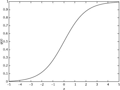
Illustration of logistic function. In logistic regression, p(Y = 1|X) is defined to follow this form.
As the sum of the probabilities must equal 1, p(Y = 0|X) can be estimated using the following equation
p(Y=0|X)=1−g(θTX)=e−θTX1+e−θTX.(3.20)
Because logistic regression predicts probabilities, rather than just classes, we can fit it using likelihood. For each training data point, we have a vector of features, X = 〈X0,X1, …,Xd〉 (X0 = 1), and an observed class, Y = Yk. The probability of that class was either g(θTX) if yk = 1, or 1 − g(θTX) if yk = 0. Note that we can combine both Equation (3.19) and Equation (3.20) as a more compact form
p(Y=yk|X;θ)=(p(Y=1|X))yk(p(Y=0|X))1−yk(3.21)
=(g(θTX))yk(1−g(θTX))1−yk.(3.22)
Assuming that the N training examples were generated independently, the likelihood of the parameters can be written as
where θ is the vector of parameters to be estimated, Y(n) denotes the observed value of Y in the nth training example, and X(n) denotes the observed value of X in the nth training example. To classify any given X, we generally want to assign the value yk to Y that maximizes the likelihood as discussed in the following subsection.
3.3.2 Parameters Estimation for Logistic Regression
In general, maximum likelihood is used to determine the parameters of the logistic regression. The conditional likelihood is the probability of the observed Y values in the training data, conditioned on their corresponding X values. We choose parameters θ that satisfy
where θ = 〈θ0,θ1, …,θd〉 is the vector of parameters to be estimated, and this model has d + 1 adjustable parameters for a d-dimensional feature space.
Maximizing the likelihood is equivalent to maximizing the log likelihood:
To estimate the vector of parameters θ, we maximize the log likelihood with the following rule
Since there is no closed form solution to maximizing l(θ) with respect to θ, we use gradient ascent [37, 38] to solve the problem. Written in vectorial notation, our updates will therefore be given by θ ← θ + α Δθl(θ). After taking partial derivatives, the ith component of the vector gradient has the form
where g(θTX(n)) is the logistic regression prediction using Equation (3.19). The term inside the parentheses can be interpreted as the prediction error, which is the difference between the observed Y(n) and its predicted probability. Note that if Y(n) = 1 then we expect g(θTX(n)) (p(Y = 1|X)) to be 1, whereas if Y(n) = 0 then we expect g(θTX(n)) to be 0, which makes p(Y = 0|X) equal to 1. This error term is multiplied by the value of , so as to take account for the magnitude of the term in making this prediction.
According to the standard gradient ascent and the derivative of each θi, we can repeatedly update the weights in the direction of the gradient as follows:
where α is a small constant (e.g., 0.01) that is called as the learning step or step size. Because the log likelihood l(θ) is a concave function in θ, this gradient ascent procedure will converge to a global maximum rather than a local maximum. The above method looks at every example in the entire training set on every step, and it is called batch gradient ascent. Another alternative method is called stochastic gradient ascent. In that method, we repeatedly run through the training set, and each time we encounter a training example, then we update the parameters according to the gradient of error with respect to that single training example only, which can be expressed as
In many cases where the computational efficiency is important, it is common to use the stochastic gradient ascent to estimate the parameters.
Besides maximum likelihood, Newton’s method [32, 39] is a different algorithm for maximizing l(θ). Newton’s method typically enjoys faster convergence than (batch) gradient descent, and requires many fewer iterations to get very close to the minimum. For more details about Newton’s method, please refer to [32].
3.3.3 Regularization in Logistic Regression
Overfitting generally occurs when a statistical model describes random error or noise instead of the underlying relationship. It is a problem that can arise in logistic regression, especially when the training data is sparse and high dimensional. A model that has been overfit will generally have poor predictive performance, as it can exaggerate minor fluctuations in the data. Regularization is an approach to reduce overfitting by adding a regularization term to penalize the log likelihood function for large values of θ. One popular approach is to add L2 norm to the log ilkelihood as follows:
which constrains the norm of the weight vector to be small. Here λ is a constant that determines the strength of the penalty term.
By adding this penalty term, it is easy to show that maximizing it corresponds to calculating the MAP estimate for θ under the assumption that the prior distribution p(θ) is a Normal distribution with mean zero, and a variance related to 1/λ. In general, the MAP estimate for θ can be written as
and if p(θ) is a zero mean Gaussian distribution, then log p(θ) yields a term proportional to ||θ||2. After taking partial derivatives, we can easily obtain the form
and the modified gradient descent rule becomes
3.3.4 Applications
Logistic regression is used extensively in numerous disciplines [26], including the Web, and medical and social science fields. For example, logistic regression might be used to predict whether a patient has a given disease (e.g., diabetes), based on observed characteristics of the patient (age, gender, body mass index, results of various blood tests, etc.) [3, 22]. Another example [2] might be to predict whether an American voter will vote Democratic or Republican, based on age, income, gender, race, state of residence, votes in previous elections, etc. The technique can also be used in engineering, especially for predicting the probability of failure of a given process, system, or product. It is also used in marketing applications such as predicting of a customer’s propensity for purchasing a product or ceasing a subscription, etc. In economics it can be used to predict the likelihood of a person’s choosing to be in the labor force, and in a business application, it would be used to predict the likelihood of a homeowner defaulting on a mortgage.
3.4 Probabilistic Graphical Models for Classification
A graphical model [13, 17] is a probabilistic model for which a graph denotes the conditional independence structure between random variables. Graphical models provide a simple way to visualize the structure of a probabilistic model and can be used to design and motivate new models. In a probabilistic graphical model, each node represents a random variable, and the links express probabilistic relationships between these variables. The graph then captures the way in which the joint distribution over all of the random variables can be decomposed into a product of factors, each depending only on a subset of the variables. There are two branches of graphical representations of distributions that are commonly used: directed and undirected. In this section, we discuss the key aspects of graphical models for classification. We will mainly cover a directed graphical model hidden Markov model (HMM), and undirected graphical model conditional random fields (CRF). In addition, we will introduce basic Bayesian networks and Markov random fields as the preliminary contents for HMM and CRF, respectively.
3.4.1 Bayesian Networks
Bayesian networks (BNs), also known as belief networks (or Bayes nets for short), belong to the directed graphical models, in which the links of the graphs have a particular directionality indicated by arrows. Formally, BNs are directed acyclic graphs (DAG) whose nodes represent random variables, and whose edges represent conditional dependencies. For example, a link from random variable X to Y can be informally interpreted as indicating that X “causes” Y. For the classification task, we can create a node for the random variable that is going to be classified, and the goal is to infer the discrete value associated with the random variable. For example, in order to classify whether a patient has lung cancer, a node representing “lung cancer” will be created together with other factors that may directly or indirectly cause lung cancer and outcomes that will be caused by lung cancer. Given the observations for other random variables in BN, we can infer the probability of a patient having lung cancer.
3.4.1.1 Bayesian Network Construction
Once the nodes are created for all the random variables, the graph structure between these nodes needs to be specified. Bayesian network assumes a simple conditional independence assumption between random variables, which can be stated as follows: a node is conditionally independent of its non-descendants given its parents, where the parent relationship is with respect to some fixed topological ordering of the nodes. This is also called local Markov property, denoted by for all v ∈ V (the notation ⊥⊥ represents “is independent of”), where de(v) is the set of descendants of v and pa(v) denotes the parent node set of v. For example, as shown in Figure 3.2(a), we obtain .
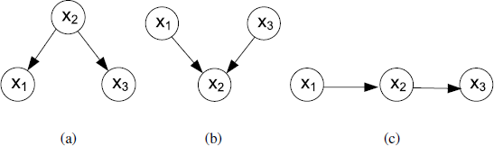
Examples of directed acyclic graphs describing the dependency relationships among variables.
One key calculation for BN is to compute the joint distribution of an observation for all the random variables, p(x). By using the chain rule of probability, the above joint distribution can be written as a product of conditional distributions, given the topological order of these random variables:
By utilizing the conditional independence assumption, the joint probability of all random variables can be factored into a product of density functions for all of the nodes in the graph, conditional on their parent variables. That is, since More precisely, for a graph with n nodes (denoted as x1, …,xn), the joint distribution is given by:
where pai is the set of parents of node xi.
Considering the graph shown in Figure 3.2, we can go from this graph to the corresponding representation of the joint distribution written in terms of the product of a set of conditional probability distributions, one for each node in the graph. The joint distributions for Figure 3.2(a)-(c) are therefore and respectively.
In addition to the graph structure, the conditional probability distribution, p(Xi|Pai), needs to be given or learned. When the random variable is discrete, this distribution can be represented using conditional probability table (CPT), which lists the probability of each value taken by Xi given all the possible configurations of its parents. For example, assuming X1, X2, and X3 in Figure 3.2(b) are all binary random variables, a possible conditional probability table for p(X2|X1,X3) could be:
X1 = 0; X3 = 0 |
X1 = 0; X3 = 1 |
X1 = 1; X3 = 0 |
X1 = 1; X3 = 1 |
|
|---|---|---|---|---|
X2 = 0 |
0.1 |
0.4 |
0.8 |
0.3 |
X2 = 1 |
0.9 |
0.6 |
0.2 |
0.7 |
3.4.1.2 Inference in a Bayesian Network
The classification problem then can be solved by computing the probability of the interested random variable (e.g., lung cancer) taking a certain class label, given the observations of other random variables, which can be calculated if the joint probability of all the variables is known:
Because a BN is a complete model for the variables and their relationships, a complete joint probability distribution (JPD) over all the variables is specified for a model. Given the JPD, we can answer all possible inference queries by summing out (marginalizing) over irrelevant variables. However, the JPD has size O(2n), where n is the number of nodes, and we have assumed each node can have 2 states. Hence summing over the JPD takes exponential time. The most common exact inference method is Variable Elimination [8]. The general idea is to perform the summation to eliminate the non-observed non-query variables one by one by distributing the sum over the product. The reader can refer to [8] for more details. Instead of exact inference, a useful approximate algorithm called Belief propagation [30] is commonly used on general graphs including Bayesian network, which will be introduced in Section 3.4.3.
3.4.1.3 Learning Bayesian Networks
The learning of Bayesian networks is comprised of two components: parameter learning and structure learning. When the graph structure is given, only the parameters such as the probabilities in conditional probability tables need to be learned given the observed data. Typically, MLE (Maximum Likelihood Estimation) or MAP (Maximum a Posterior) estimations will be used to find the best parameters. If the graph structure is also unknown, both the graph structure and the parameters need to be learned from the data.
From the data point of view, it could be either complete or incomplete, depending on whether all the random variables are observable. When hidden random variables are involved, EM algorithms are usually used.
3.4.2 Hidden Markov Models
We now introduce a special case of Bayesian network, the hidden Markov model. In a hidden Markov model, hidden states are linked as a chain and governed by a Markov process; and the observable values are independently generated given the hidden state, which form a sequence. Hidden Markov model is widely used in speech recognition, gesture recognition, and part-of-speech tagging, where the hidden classes are dependent on each other. Therefore, the class labels for an observation are not only dependent on the observation but also dependent on the adjacent states.
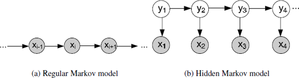
In a regular Markov model as Figure 3.3(a), the state xi is directly visible to the observer, and therefore the state transition probabilities p(xi|xi-1) are the only parameters. Based on the Markov property, the joint distribution for a sequence of n observations under this model is given by
Thus, if we use such a model to predict the next observation in a sequence, the distribution of predictions will depend on the value of the immediately preceding observation and will be independent of all earlier observations, conditional on the preceding observation.
A hidden Markov model (HMM) can be considered as the simplest dynamic Bayesian network. In a hidden Markov model, the state yi is not directly visible, and only the output xi, dependent on the state, is visible. The hidden state space is discrete, and is assumed to consist of one of N possible values, which is also called latent variable. The observations can be either discrete or continuous, and are typically generated from a categorical distribution or a Gaussian distribution. Generally, an HMM can be considered as a generalization of a mixture model where the hidden variables are related through a Markov process rather than independent of each other.
Suppose the latent variables form a first-order Markov chain as shown in Figure 3.3(b). The random variable yt is the hidden state at time t, and the random variable xt is the observation at time t. The arrows in the figure denote conditional dependencies. From the diagram, it is clear that yt-1 and yt+1 are independent given yt, so This is the key conditional independence property, which is called the Markov property. Similarly, the value of the observed variable xt only depends on the value of the hidden variable yt. Then, the joint distribution for this model is given by
where p(yt |yt-1) is the state transition probability, and p(xt |yt) is the observation probability.
3.4.2.1 The Inference and Learning Algorithms
Consider the case where we are given a set of possible states ΩY = {q1, …,qN} and a set of possible observations ΩX = {o1, …,oM}. The parameter learning task of HMM is to find the best set of state transition probabilities and observation probabilities as well as the initial state distribution for a set of output sequences. Let Λ = {A,B, ∏} denote the parameters for a given HMM with fixed ΩY and ΩX. The task is usually to derive the maximum likelihood estimation of the parameters of the HMM given the set of output sequences. Usually a local maximum likelihood can be derived efficiently using the Baum-Welch algorithm [4], which makes use of forward-backward algorithm [33], and is a special case of the generalized EM algorithm [9].
Given the parameters of the model Λ, there are several typical inference problems associated with HMMs, as outlined below. One common task is to compute the probability of a particular output sequence, which requires summation over all possible state sequences: The probability of observing a sequence of length T is given by where the sum runs over all possible hidden-node sequences
This problem can be handled efficiently using the forward-backward algorithm. Before we describe the algorithm, let us define the forward (alpha) values and backward (beta) values as follows: and Note the forward values enable us to solve the problem through marginalizing, then we obtain
The forward values can be computed efficiently with the principle of dynamic programming:
Similarly, the backward values can be computed as
The backward values will be used in the Baum-Welch algorithm.
Given the parameters of HMM and a particular sequence of observations, another interesting task is to compute the most likely sequence of states that could have produced the observed sequence. We can find the most likely sequence by evaluating the joint probability of both the state sequence and the observations for each case. For example, in Part-of-speech (POS) tagging [18], we observe a token (word) sequence and the goal of POS tagging is to find a stochastic optimal tag sequence that maximizes . In general, finding the most likely explanation for an observation sequence can be solved efficiently using the Viterbi algorithm [12] by the recurrence relations:
Here Vt(j) is the probability of the most probable state sequence responsible for the first t observations that has qj as its final state. The Viterbi path can be retrieved by saving back pointers that remember which state yt = qj was used in the second equation. Let Ptr(yt, qi) be the function that returns the value of yt-1 used to compute Vt (i) as follows:
The complexity of this algorithm is O(T × N2), where T is the length of observed sequence and N is the number of possible states.
Now we need a method of adjusting the parameters Λ to maximize the likelihood for a given training set. The Baum-Welch algorithm [4] is used to find the unknown parameters of HMMs, which is a particular case of a generalized EM algorithm [9]. We start by choosing arbitrary values for the parameters, then compute the expected frequencies given the model and the observations. The expected frequencies are obtained by weighting the observed transitions by the probabilities specified in the current model. The expected frequencies obtained are then substituted for the old parameters and we iterate until there is no improvement. On each iteration we improve the probability of being observed from the model until some limiting probability is reached. This iterative procedure is guaranteed to converge on a local maximum [34].
3.4.3 Markov Random Fields
Now we turn to another major class of graphical models that are described by undirected graphs and that again specify both a factorization and a set of conditional independence relations. A Markov random field (MRF), also known as an undirected graphical model [14], has a set of nodes, each of which corresponds to a variable or group of variables, as well as a set of links, each of which connects a pair of nodes. The links are undirected, that is, they do not carry arrows.
3.4.3.1 Conditional Independence
Given three sets of nodes, denoted A, B, and C, in an undirected graph G, if A and B are separated in G after removing a set of nodes C from G, then A and B are conditionally independent given the random variables C, denoted as The conditional independence is determined by simple graph separation. In other words, a variable is conditionally independent of all other variables given its neighbors, denoted as where ne(v) is the set of neighbors of v. In general, an MRF is similar to a Bayesian network in its representation of dependencies, and there are some differences. On one hand, an MRF can represent certain dependencies that a Bayesian network cannot (such as cyclic dependencies); on the other hand, MRF cannot represent certain dependencies that a Bayesian network can (such as induced dependencies).
3.4.3.2 Clique Factorization
As the Markov properties of an arbitrary probability distribution can be difficult to establish, a commonly used class of MRFs are those that can be factorized according to the cliques of the graph. A clique is defined as a subset of the nodes in a graph such that there exists a link between all pairs of nodes in the subset. In other words, the set of nodes in a clique is fully connected.
We can therefore define the factors in the decomposition of the joint distribution to be functions of the variables in the cliques. Let us denote a clique by C and the set of variables in that clique by xC. Then the joint distribution is written as a product of potential functions ψC(xC) over the maximal cliques of the graph
where the partition function Z is a normalization constant and is given by In contrast to the factors in the joint distribution for a directed graph, the potentials in an undirected graph do not have a specific probabilistic interpretation. Therefore, how to motivate a choice of potential function for a particular application seems to be very important. One popular potential function is defined as where is an energy function [29] derived from statistical physics. The underlying idea is that the probability of a physical state depends inversely on its energy. In the logarithmic representation, we have
The joint distribution above is defined as the product of potentials, and so the total energy is obtained by adding the energies of each of the maximal cliques.
A log-linear model is a Markov random field with feature functions fk such that the joint distribution can be written as
where fk(xCk) is the function of features for the clique Ck, and λk is the weight vector of features. The log-linear model provides a much more compact representation for many distributions, especially when variables have large domains such as text.
3.4.3.3 The Inference and Learning Algorithms
In MRF, we may compute the conditional distribution of a set of nodes given values A to another set of nodes B by summing over all possible assignments to v ∉A, B, which is called exact inference. However, the exact inference is computationally intractable in the general case. Instead, approximation techniques such as MCMC approach [1] and loopy belief propagation [5, 30] are often more feasible in practice. In addition, there are some particular subclasses of MRFs that permit efficient Maximum a posterior (MAP) estimation, or more likely, assignment inference, such as associate networks. Here we will briefly describe belief propagation algorithm.
Belief propagation is a message passing algorithm for performing inference on graphical models, including Bayesian networks and MRFs. It calculates the marginal distribution for each unobserved node, conditional on any observed nodes. Generally, belief propagation operates on a factor graph, which is a bipartite graph containing nodes corresponding to variables V and factors U, with edges between variables and the factors in which they appear. Any Bayesian network and MRF can be represented as a factor graph. The algorithm works by passing real valued function called messages along the edges between the nodes. Taking pairwise MRF as an example, let mij(xj) denote the message from node i to node j, and a high value of mij(xj) means that node i “believes” the marginal value P(xj) to be high. Usually the algorithm first initializes all messages to uniform or random positive values, and then updates message from i to j by considering all messages flowing into i (except for message from j) as follows:
where fij(xi,xj) is the potential function of the pairwise clique. After enough iterations, this process is likely to converge to a consensus. Once messages have converged, the marginal probabilities of all the variables can be determined by
The reader can refer to [30] for more details. The main cost is the message update equation, which is O(N2) for each pair of variables (N is the number of possible states).
Recently, MRF has been widely used in many text mining tasks, such as text categorization [7] and information retrieval [28]. In [28], MRF is used to model the term dependencies using the joint distribution over queries and documents. The model allows for arbitrary text features to be incorporated as evidence. In this model, an MRF is constructed from a graph G, which consists of query nodes qi and a document node D. The authors explore full independence, sequential dependence, and full dependence variants of the model. Then, a novel approach is developed to train the model that directly maximizes the mean average precision. The results show significant improvements are possible by modeling dependencies, especially on the larger Web collections.
3.4.4 Conditional Random Fields
So far, we have described the Markov network representation as a joint distribution. One notable variant of an MRF is a conditional random field (CRF) [19, 40], in which each variable may also be conditioned upon a set of global observations. More formally, a CRF is an undirected graph whose nodes can be divided into exactly two disjoint sets, the observed variables X and the output variables Y, which can be parameterized as a set of factors in the same way as an ordinary Markov network. The underlying idea is that of defining a conditional probability distribution p(Y|X) over label sequences Y given a particular observation sequence X, rather than a joint distribution over both label and observation sequences p(Y,X). The primary advantage of CRFs over HMMs is their conditional nature, resulting in the relaxation of the independence assumptions required by HMMs in order to ensure tractable inference.
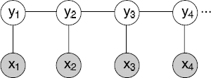
Considering a linear-chain CRF with Y = {y1,y2, …,yn} and X = {x1,x2, …, xn} as shown in Figure 3.4, an input sequence of observed variable X represents a sequence of observations and Y represents a sequence of hidden state variables that needs to be inferred given the observations. The yi’s are structured to form a chain, with an edge between each yi and yi+1. The distribution represented by this network has the form:
where Z(X) =
3.4.4.1 The Learning Algorithms
For general graphs, the problem of exact inference in CRFs is intractable. Basically, the inference problem for a CRF is the same as for an MRF. If the graph is a chain or a tree, as shown in Figure 3.4, message passing algorithms yield exact solutions, which are similar to the forward-backward [4, 33] and Viterbi algorithms [12] for the case of HMMs. If exact inference is not possible, generally the inference problem for a CRF can be derived using approximation techniques such as MCMC [1, 31], loopy belief propagation [5, 30], and so on. Similar to HMMs, the parameters are typically learned by maximizing the likelihood of training data. It can be solved using an iterative technique such as iterative scaling [19] and gradient-descent methods [37].
CRF has been applied to a wide variety of problems in natural language processing, including POS tagging [19], shallow parsing [37], and named entity recognition [24], being an alternative to the related HMMs. Based on HMM models, we can determine the sequence of labels by maximizing a joint probability distribution p(X,Y). In contrast, CRMs define a single log-linear distribution, i.e., p(Y|X), over label sequences given a particular observation sequence. The primary advantage of CRFs over HMMs is their conditional nature, resulting in the relaxation of the independence assumptions required by HMMs in order to ensure tractable inference. As expected, CRFs outperform HMMs on POS tagging and a number of real-word sequence labeling tasks [19, 24].
3.5 Summary
This chapter has introduced the most frequently used probabilistic models for classification, which include generative probabilistic classifiers, such as naive Bayes classifiers and hidden Markov models, and discriminative probabilistic classifiers, such as logistic regression and conditional random fields. Some of the classifiers, like the naive Bayes classifier, may be more appropriate for high-dimensional text data, whereas others such as HMM and CRF are used more commonly for temporal or sequential data. The goal of learning algorithms for these probabilistic models are to find MLE or MAP estimations for parameters in these models. For simple naive Bayes classifier and logistic regression, there are closed form solutions for them. In other cases, iterative algorithms such as the gradient-descent method are good options.
Bibliography
[1] C. Andrieu, N. De Freitas, A. Doucet, and M. Jordan. An introduction to mcmc for machine learning. Machine Learning, 50(1):5–43, 2003.
[2] J. Antonakis and O. Dalgas. Predicting elections: Child’s play! Science, 323(5918):1183–1183, 2009.
[3] S. C. Bagley, H. White, and B. A. Golomb. Logistic regression in the medical literature: Standards for use and reporting, with particular attention to one medical domain. Journal of Clinical Epidemiology, 54(10):979–985, 2001.
[4] L. Baum, T. Petrie, G. Soules, and N. Weiss. A maximization technique occurring in the statistical analysis of probabilistic functions of Markov chains. The Annals of Mathematical Statistics, 41(1):164–171, 1970.
[5] C. Bishop. Pattern Recognition and Machine Learning, volume 4. Springer New York, 2006.
[6] S. F. Chen and J. Goodman. An empirical study of smoothing techniques for language modeling. In Proceedings of the 34th Annual Meeting on Association for Computational Linguistics, pages 310–318. Association for Computational Linguistics, 1996.
[7] S. Chhabra, W. Yerazunis, and C. Siefkes. Spam filtering using a Markov random field model with variable weighting schemas. In Proceedings of the 4th IEEE International Conference on Data Mining, 2004. ICDM’04, pages 347–350, 2004.
[8] F. Cozman. Generalizing variable elimination in Bayesian networks. In Workshop on Probabilistic Reasoning in Artificial Intelligence, pages 27–32. 2000.
[9] A. P. Dempster, N. M. Laird, and D. B. Rubin. Maximum likelihood from incomplete data via the em algorithm. Journal of the Royal Statistical Society. Series B, 39(1): 1–38, 1977.
[10] P. Domingos and M. Pazzani. On the optimality of the simple Bayesian classifier under zero-one loss. Machine Learning, 29(2–3):103–130, 1997.
[11] R. O. Duda and P. E. Hart. Pattern Classification and Scene Analysis, volume 3. Wiley New York, 1973.
[12] G. Forney Jr. The viterbi algorithm. Proceedings of the IEEE, 61(3):268–278, 1973.
[13] M. I. Jordan. Graphical models. Statistical Science, 19(1):140–155, 2004.
[14] R. Kindermann, J. Snell, and American Mathematical Society. Markov Random Fields and Their Applications. American Mathematical Society Providence, RI, 1980.
[15] D. Kleinbaum and M. Klein. Maximum likelihood techniques: An overview. Logistic regression, pages 103–127, 2010.
[16] R. Kohavi. Scaling up the accuracy of Naive-Bayes classifiers: A decision-tree hybrid. In KDD, pages 202–207, 1996.
[17] D. Koller and N. Friedman. Probabilistic graphical models. MIT Press, 2009.
[18] J. Kupiec. Robust part-of-speech tagging using a hidden markov model. Computer Speech & Language, 6(3):225–242, 1992.
[19] J. D. Lafferty, A. McCallum, and F. C. N. Pereira. Conditional random fields: Probabilistic models for segmenting and labeling sequence data. In ICML, pages 282–289, 2001.
[20] P. Langley, W. Iba, and K. Thompson. An analysis of Bayesian classifiers. In AAAI, volume 90, pages 223–228, 1992.
[21] D. D. Lewis. Naive (Bayes) at forty: The independence assumption in information retrieval. In ECML, pages 4–15, 1998.
[22] J. Liao and K.-V. Chin. Logistic regression for disease classification using microarray data: Model selection in a large p and small n case. Bioinformatics, 23(15): 1945–1951, 2007.
[23] P. MacCullagh and J. A. Nelder. Generalized Linear Models, volume 37. CRC Press, 1989.
[24] A. McCallum and W. Li. Early results for named entity recognition with conditional random fields, feature induction and web-enhanced lexicons. In Proceedings of the 7th Conference on Natural Language Learning at HLT-NAACL 2003-Volume 4, pages 188–191, ACL, 2003.
[25] A. McCallum, K. Nigam, et al. A comparison of event models for Naive Bayes text classification. In AAAI-98 Workshop on Learning for Text Categorization, volume 752, pages 41–48. 1998.
[26] S. Menard. Applied Logistic Regression Analysis, volume 106. Sage, 2002.
[27] V. Metsis, I. Androutsopoulos, and G. Paliouras. Spam filtering with Naive Bayes—Which Naive Bayes? In Third Conference on Email and Anti-Spam, pp. 27–28, 2006.
[28] D. Metzler and W. Croft. A Markov random field model for term dependencies. In Proceedings of the 28th Annual International ACM SIGIR Conference on Research and Development in Information Retrieval, pages 472–479. ACM, 2005.
[29] T. Minka. Expectation propagation for approximate Bayesian inference. In Uncertainty in Artificial Intelligence, volume 17, pages 362–369. 2001.
[30] K. Murphy, Y. Weiss, and M. Jordan. Loopy belief propagation for approximate inference: An empirical study. In Proceedings of the Fifteenth Conference on Uncertainty in AI, volume 9, pages 467–475, 1999.
[31] R. M. Neal. Markov chain sampling methods for dirichlet process mixture models. Journal of Computational and Graphical Statistics, 9(2):249–265, 2000.
[32] L. Qi and J. Sun. A nonsmooth version of Newton’s method. Mathematical Programming, 58(1–3):353–367, 1993.
[33] L. Rabiner. A tutorial on hidden Markov models and selected applications in speech recognition. Proceedings of the IEEE, 77(2):257–286, 1989.
[34] L. R. Rabiner and B. H. Juang. An introduction to hidden Markov models. IEEE ASSP Magazine, 3(1): 4–15, January 1986.
[35] I. Rish. An empirical study of the naive bayes classifier. In IJCAI 2001 Workshop on Empirical Methods in Artificial Intelligence, pages 41–46, 2001.
[36] I. Rish, J. Hellerstein, and J. Thathachar. An analysis of data characteristics that affect Naive Bayes performance. In Proceedings of the Eighteenth Conference on Machine Learning, 2001.
[37] F. Sha and F. Pereira. Shallow parsing with conditional random fields. In Proceedings of the 2003 Conference of the North American Chapter of the Association for Computational Linguistics on Human Language Technology, pages 134–141. 2003.
[38] J. A. Snyman. Practical Mathematical Optimization: An Introduction to Basic Optimization Theory and Classical and New Gradient-Based Algorithms, volume 97. Springer, 2005.
[39] J. Stoer, R. Bulirsch, R. Bartels, W. Gautschi, and C. Witzgall. Introduction to Numerical Analysis, volume 2. Springer New York, 1993.
[40] C. Sutton and A. McCallum. An introduction to conditional random fields for relational learning. In Introduction to Statistical Relational Learning, L. Getoor and B. Taskar(eds.) pages 95–130, MIT Press, 2006.