Chapter 19

Ensemble Learning

Yaliang Li

State University of New York at Buffalo
Buffalo, NY
[email protected]

Jing Gao

State University of New York at Buffalo
Buffalo, NY
[email protected]

Qi Li

State University of New York at Buffalo
Buffalo, NY
[email protected]

Wei Fan

Huawei Noah’s Ark Lab
Hong Kong
[email protected]

19.1 Introduction

People have known the benefits of combining information from multiple sources since a long time ago. From the old story of “blind men and an elephant,” we can learn the importance of capturing a big picture instead of focusing on one single perspective. In the story, a group of blind men touch different parts of an elephant to learn what it is like. Each of them makes a judgment about the elephant based on his own observation. For example, the man who touched the ear said it was like a fan while the man who grabbed the tail said it was like a rope. Clearly, each of them just got a partial view and did not arrive at an accurate description of the elephant. However, as they captured different aspects about the elephant, we can learn the big picture by integrating the knowledge about all the parts together.

Ensemble learning can be regarded as applying this “crowd wisdom” to the task of classification. Classification, or supervised learning, tries to infer a function that maps feature values into class labels from training data, and apply the function to data with unknown class labels. The function is called a model or classifier. We can regard a collection of some possible models as a hypothesis space H, and each single point h ∈ H in this space corresponds to a specific model. A classification algorithm usually makes certain assumptions about the hypothesis space and thus defines a hypothesis space to search for the correct model. The algorithm also defines a certain criterion to measure the quality of the model so that the model that has the best measure in the hypothesis space will be returned. A variety of classification algorithms have been developed [8], including Support Vector Machines [20, 22], logistic regression [47], Naive Bayes, decision trees [15, 64, 65], k-nearest neighbor algorithm [21], and Neural Networks [67, 88]. They differ in the hypothesis space, model quality criteria and search strategies.

In general, the goal of classification is to find the model that achieves good performance when predicting the labels of future unseen data. To improve the generalization ability of a classification model, it should not overfit the training data; instead, it should be general enough to cover unseen cases. Ensemble approaches can be regarded as a family of classification algorithms, which are developed to improve the generalization abilities of classifiers. It is hard to get a single classification model with good generalization ability, which is called a strong classifier, but ensemble learning can transform a set of weak classifiers into a strong one by their combination. Formally, we learn T classifiers from a training set D: {h1(x),…, hT(x)}, each of which maps feature values x into a class label y. We then combine them into an ensemble classifier H(x) with the hope that it achieves better performance.

There are two major factors that contribute to the success of ensemble learning. First, theoretical analysis and real practice have shown that the expected error of an ensemble model is smaller than that of a single model. Intuitively, if we know in advance that h1(x) has the best prediction performance on future data, then without any doubt, we should discard the other classifiers and choose h1(x) for future predictions. However, we do not know the true labels of future data, and thus we are unable to know in advance which classifier performs the best. Therefore, our best bet should be the prediction obtained by combining multiple models. This simulates what we do in real life—When making investments, we will seldom rely on one single option, but rather distribute the money across multiple stocks, plans, and accounts. This will usually lead to lower risk and higher gain. In many other scenarios, we will combine independent and diverse opinions to make better decisions.

A simple example can be used to further illustrate how the ensemble model achieves better performance [74]. Consider five completely independent classifiers and suppose each classifier has a prediction accuracy of 70% on future data. If we build an ensemble classifier by combining these five classifiers using majority voting, i.e., predict the label as the one receiving the highest votes among classifiers, then we can compute the probability of making accurate classification as: 10 × 0.73 × 0.32 + 5 × 0.74 × 0.3 + 0.75 = 83.7% (the sum of the probability of having 3, 4, and 5 classifiers predicting correctly). If we now have 101 such classifiers, following the same principle, we can derive that the majority voting approach on 101 classifiers can reach an accuracy of 99.9%. Clearly, the ensemble approach can successfully cancel out independent errors made by individual classifiers and thus improve the classification accuracy.

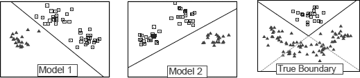
Another advantage of ensemble learning is its ability to overcome the limitation of hypothesis space assumption made by single models. As discussed, a single-model classifier usually searches for the best model within a hypothesis space that is assumed by the specific learning algorithm. It is very likely that the true model does not reside in the hypothesis space, and then it is impossible to obtain the true model by the learning algorithm. Figure 19.1 shows a simple example of binary classification. The rightmost plot shows that the true decision boundary is V-shaped, but if we search for a classifier within a hypothesis space consisting of all the linear classifiers, for example, models 1 and 2, we are unable to recover the true boundary. However, by combining multiple classifiers, ensemble approaches can successfully simulate the true boundary. The reason is that ensemble learning methods combine different hypotheses and the final hypothesis is not necessarily contained in the original hypothesis space. Therefore, ensemble methods have more flexibility in the hypothesis they could represent.

Due to these advantages, many ensemble approaches [4, 23, 52, 63, 74, 75, 90] have been developed to combine complementary predictive power of multiple models. Ensemble learning is demonstrated as useful in many data mining competitions (e.g., Netflix contest,1 KDD cup,2 ICDM con-test3) and real-world applications. There are two critical components in ensemble learning: Training base models and learning their combinations, which are discussed as follows.

From the majority voting example we mentioned, it is obvious that the base classifiers should be accurate and independent to obtain a good ensemble. In general, we do not require the base models to be highly accurate—as long as we have a good amount of base classifiers, the weak classifiers can be boosted to a strong classifier by combination. However, in the extreme case where each classifier is terribly wrong, the combination of these classifiers will give even worse results. Therefore, at least the base classifiers should be better than random guessing. Independence among classifiers is another important property we want to see in the collection of base classifiers. If base classifiers are highly correlated and make very similar predictions, their combination will not improve anymore. In contrast, when base classifiers are independent and make diverse predictions, the independent errors have better chances to be canceled out. Typically, the following techniques have been used to generate a good set of base classifiers:

• Obtain different bootstrap samples from the training set and train a classifier on each bootstrap sample;
• Extract different subsets of examples or subsets of features and train a classifier on each subset;
• Apply different learning algorithms on the training set;
• Incorporate randomness into the process of a particular learning algorithm or use different parametrization to obtain different prediction results.

To further improve the accuracy and diversity of base classifiers, people have explored various ways to prune and select base classifiers. More discussions about this can be found in Section 19.6.

Once the base classifiers are obtained, the important question is how to combine them. The combination strategies used by ensemble learning methods roughly fall into two categories: Unweighted and weighted. Majority voting is a typical un-weighted combination strategy, in which we count the number of votes for each predicted label among the base classifiers and choose the one with the highest votes as the final predicted label. This approach treats each base classifier as equally accurate and thus does not differentiate them in the combination. On the other hand, weighted combination usually assigns a weight to each classifier with the hope that higher weights are given to more accurate classifiers so that the final prediction can bias towards the more accurate classifiers. The weights can be inferred from the performance of base classifiers or the combined classifier on the training set.

In this book chapter, we will provide an overview of the classical ensemble learning methods discussing their base classifier generation and combination strategies. We will start with Bayes optimal classifier, which considers all the possible hypotheses in the whole hypothesis space and combines them. As it cannot be practically implemented, two approximation methods, i.e., Bayesian model averaging and Bayesian model combination, have been developed (Section 19.2). In Section 19.3, we discuss the general idea of bagging, which combines classifiers trained on bootstrap samples using majority voting. Random forest is then introduced as a variant of bagging. In Section 19.4, we discuss the boosting method, which gradually adjusts the weights of training examples so that weak classifiers can be boosted to learn accurately on difficult examples. AdaBoost will be introduced as a representative of the boosting method. Stacking is a successful technique to combine multiple classifiers, and its usage in top performers of the Netflix competition has attracted much attention to this approach. We discuss its basic idea in Section 19.5. After introducing these classical approaches, we will give a brief overview of recent advances in ensemble learning, including new ensemble learning techniques, ensemble pruning and selection, and ensemble learning in various challenging learning scenarios. Finally, we conclude the book chapter by discussing possible future directions in ensemble learning. The notations used throughout the book chapter are summarized in

19.2 Bayesian Methods

In this section, we introduce Bayes optimal classification and its implementation approaches including Bayesian model averaging and Bayesian model combination.

19.2.1 Bayes Optimal Classifier

Ensemble methods try to combine different models into one model in which each base model is assigned a weight based on its contribution to the classification task. As we discussed in the Introduction, two important questions in ensemble learning are: Which models should be considered and how to choose them from the hypothesis space? How to assign the weight to each model? One natural solution is to consider all the possible hypotheses in the hypothesis space and infer model weights from training data. This is the basic principle adopted by the Bayes optimal classifier.

Specifically, given a set of training data $\mathcal{D}={\left\{{\text{x}}_i,y_i\right\}}_{i=1}^m$, where xi ∈ ℝn and yi ∈ Y, our goal is to obtain an ensemble classifier that assigns a label to unseen data x in the following way:

$$\begin{array}{ccc}y=\underset{yϵ\mathcal{Y}}{\arg \max }{\displaystyle \sum _{hϵ\mathscr{H}}p\left(y|\text{x,}h\right)p\left(h|\mathcal{D}\right)}.& & \left(19.1\right)\end{array}$$

In this equation, y is the predicted label of x, Y is the set of all possible labels, H is the hypothesis space that contains all possible hypothesis h, and p() denotes probability functions. We can see that the Bayes optimal classifier combines all possible base classifiers, i.e., the hypotheses, by summing up their weighted votes. The posterior probability p(h|D) is adopted to be their corresponding weights.

We assume that training examples are drawn independently. By Bayes’ theorem, the posterior probability p(h|D) is given by:

$$\begin{array}{ccc}P\left(h|\mathcal{D}\right)=\frac{p\left(h\right)p\left(\mathcal{D}|h\right)}{p\left(\mathcal{D}\right)}=\frac{p\left(h\right){\Pi }_{i=1}^{m}p\left({\text{x}}_i|h\right)}{p\left(\mathcal{D}\right)}& & \left(19.2\right)\end{array}$$

In this equation, p(h) is the prior probability reflecting the degree of our belief that h is the “correct” model prior to seeing any data. $p\left(\mathcal{D}|h\right)={\Pi }_{i=1}^{m}p\left({\text{x}}_i|h\right)$ is the likelihood, i.e., how likely the given training set is generated under the model h. The data prior p(D) is the same for all hypotheses, so it could be ignored when making the label predictions.

To sum up, Bayes optimal classifier makes a prediction for x as follows:

$$\begin{array}{ccc}y=\underset{yϵ\mathcal{Y}}{\arg \max }{\displaystyle \sum _{hϵ\mathscr{H}}p\left(y|\mathbf{\text{x,}}h\right)p\left(\mathcal{D}|h\right)p\left(h\right)}.& & \left(19.3\right)\end{array}$$

By this approach, all the models are combined by considering both prior knowledge and data likelihood. In other words, the Bayes optimal classifier combines all the hypotheses in the hypothesis space, and each hypothesis is given a weight reflecting the probability that the training data would be sampled under the hypothesis if that hypothesis were true. In [61], it is pointed out that Bayes optimal classifier can reach optimal classification results under Bayes theorem, and on average, no other ensemble method can outperform it.

Although Bayes optimal classifier is the ideal ensemble method, unfortunately, it cannot be practically implemented. The prior knowledge about each model p(h) is usually unknown. For most tasks, the hypothesis space is too large to iterate over and many hypotheses only output a predicted label rather than a probability. Even though in some classification algorithms, it is possible to estimate the probability from training data, computing an unbiased estimate of the probability of the training data given a hypothesis, i.e., p(D|h), is difficult. The reason is that when we calculate p(xi|h), we usually have some assumptions that could be biased. Therefore, in practice, some algorithms have been developed to approximate Bayes optimal classifier. Next, we will discuss two popular algorithms, i.e., Bayesian model averaging and Bayesian model combination, which effectively implement the basic principles of Bayes optimal classifier.

19.2.2 Bayesian Model Averaging

Bayesian model averaging [46] approximates Bayes optimal classifier by combining a set of sampled models from the hypothesis space. Models are typically sampled using a Monte Carlo sampling technique. Or a simpler way is to use the model trained on a random subset of training data as a sampled model.

From Equation 19.3, we notice that there are two probabilities to compute: One is the prior probability p(h), and the other is the likelihood p(D|h). When no prior knowledge is available, we simply use uniform distribution without normalization, i.e., p(h) = 1 for all hypotheses. As for the likelihood, we can infer it based on the hypothesis’s performance on training data. Assume that the error rate of hypothesis h is E(h), then the following equation is used to compute each training example’s probability given h:

$$p\left({\text{x}}_i|h\right)=\exp \left\{\text{ε}\left(h\right)\log \left(\text{ε}\left(h\right)\right)+\left(1-\text{ε}\left(h\right)\right)\log \left(1-\text{ε}\left(h\right)\right)\right\}.$$

Suppose the size of the random subset of training data is m′, then we can get

$$p\left({\mathcal{D}}_t|h\right)=\exp \left\{m^{\prime }.\left(\text{ε}\left(h\right)\log \text{ε}\left(h\right)\right)+\left(1-\text{ε}\left(h\right)\right)\log \left(1-\text{ε}\left(h)\right)\right)\right\}.$$

Bayesian model averaging algorithm is shown in Algorithm 19.1 [1]. In [42], it was proved that when the representative hypotheses are drawn and averaged using the Bayes theorem, Bayesian model averaging has an expected error that is bounded to be at most twice the expected error of the Bayes optimal classifier.

 1: for t ← r 1 to T do

 2: Construct a subset of training data Dt with size m′ by randomly sampling in D

 3: Learn a base classifier ht based on Dt

 4: Set the prior probability p(ht) = 1

 5: Calculate ht’s error rate for predicting on Dt, which is denoted as E(ht)

 6: Calculate the likelihood $p\left({\mathcal{D}}_t|h\right)=\exp \left\{m^{\prime }.\left(\text{ε}\left(h\right)\right)\log \left(1-\text{ε}\left(h\right)\right)\log \left(1-\text{ε}\left(h)\right)\right)\right\}$

 7: Weight of ht is set as weight(ht) = p(Dt|h)p(h)

 8: end for

 9: Normalize all the weights to sum to 1

10: return $H\left(\text{x}\right)=\arg {\max }_{y\in \mathcal{Y}}{\sum }_{t=1}^{T}p\left(y|\text{x,}h\right)\cdot weight\left(h_t\right)$

Despite its theoretical correctness, Bayesian model averaging may encounter over-fitting problems. Bayesian model averaging prefers the hypothesis that by chance has the lowest error on training data rather than the hypothesis that truly has the lowest error [26]. In fact, Bayesian model averaging conducts a selection of classifiers instead of combining them. As the uniform distribution is used to set the prior probability, the weight of each base classifier is equivalent to its likelihood on training data. Typically, none of these base classifiers can fully characterize the training data, so most of them receive a small value for the likelihood term. This may not be a problem if base classifiers are exhaustively sampled from the hypothesis space, but this is rarely possible when we have limited training examples. Due to the normalization, the base classifier that captures data distribution the best will receive the largest weight and has the highest impact on the ensemble classifier. In most cases, this classifier will dominate the output and thus Bayesian model averaging conducts model selection in this sense.

Example. We demonstrate Bayesian model averaging step by step using the following example. Suppose we have a training set shown in Table 19.2, which contains 10 examples with 1-dimensional feature values and corresponding class labels (+1 or −1).

We use a set of simple classifiers that only use a threshold to make class predictions: If x is above a threshold, it is classified into one class; if it is on or below the threshold, it is classified into the other class. By learning from the training data, the classifier will decide the optimal θ (the decision boundary) and the class labels to be assigned to the two sides so that the error rate will be minimized.

We run the algorithm for five rounds using m′ = 5. Altogether we construct five training sets from the original training set and each of them contains five randomly selected examples. We first learn a base classifier ht based on each sampled training set, and then calculate its training error rate ε(ht), the likelihood p(Dt|h) and weight(ht) using the formula described in Algorithm 19.1. Table 19.3 shows the training data for each round and the predicted labels on the selected examples made by the base classifiers.

Based on the model output shown in Table 19.3, an ensemble classifier can be constructed by following Bayesian model averaging and its prediction results are shown in Table 19.4.

The highlighted points are incorrectly classified. Thus, the ensemble classifier has an error rate of 0.3. It is in fact the same classifier we obtained from Rounds 2 and 5. The weights of these two base classifiers are so high that the influence of the others is ignored in the final combination. Some techniques have been proposed to solve this dominating weight problem, for example, the Bayesian model combination method that will be discussed next.

19.2.3 Bayesian Model Combination

To overcome the over-fitting problem of Bayesian model averaging, Bayesian model combination directly samples from the space of possible ensemble hypotheses instead of sampling each hypothesis individually. By applying this strategy, Bayesian model combination finds the combination of base classifiers that simulates the underlying distribution of training data the best. This is different from Bayesian model averaging, which selects one base classifier with the best performance on training data.

The procedure of Bayesian model combination is similar to that of Bayesian model averaging. The only difference is that Bayesian model combination regards all the base classifiers as one model and iteratively calculates their weights simultaneously. The details of this algorithm can be found in Algorithm 19.2 [1]. Although Bayesian model combination is more computationally costly compared with Bayesian model averaging, it gives better results in general [62].

 1: for t ← l to T do

 2: Construct a subset of training data Dt with size m′ by randomly sampling in D

 3: Learn a base classifier ht based on Dt

 4: Set the initial weight weight(ht)= 0

 5: end for

 6: SumWeight = 0

 7: z = − ∞ (used to maintain numerical stability)

 8: Set the iteration number for computing weights: iteration

 9: for iter ← 1 to iteration do

10: For each weak classifier, draw a temp weight

11: Normalize TempWeight to sum to 1

12: Combine the base classifiers as $H^{\prime }={\sum }_{t=1}^T{h}_t\cdot TempWeight\left(h_t\right)$

13: Calculate the error rate of H′ for predicting the data in D

14: Calculate the likelihood

15: if p(D|H′) > z then

16:  For each base classifier, $weight\left(h_t\right)=weight\left(h_t\right)\exp \left\{z-p\left(\mathcal{D}|H^{\prime }\right)\right\}$

17:  z = p(D|H′)

18: end if

19: w = exp{p(D|H′) − z}

20: For each base classifier $weight\left(h_t\right)=weight\left(h_t\right)\frac{SumWeight}{SumWeight+w}+w\cdot TempWeight\left(h_t\right)$

21: SumWeight = SumWeight + w

22: end for

23: Normalize all the weights to sum to 1

24: return $H\left(\text{x}\right)=\arg {\max }_{y\in \mathcal{Y}}{\sum }_{t=1}^{T}p\left(y|\text{x,}h\right)\cdot weight\left(h_t\right)$

Example. We demonstrate how Bayesian Model Combination works using the same example in Table 19.2. In order to compare with Bayesian model averaging, we use the same random samples and the same base classifiers. We set iteration = 3. At each iteration, we draw a temp weight and normalize it (Table 19.5). Then, we combine the base classifiers by their temp weights and calculate the likelihood (shown in Table 19.6). We update weight(ht) as described in Algorithm 19.2 (Table 19.7).

It is clear that Bayesian model combination incurs more computation compared with Bayesian model averaging. Instead of sampling each hypothesis individually, Bayesian model combination samples from the space of possible ensemble hypotheses. It needs to compute an ensemble classifier and update several sets of parameters during one iteration. Weight final shows the normalized Weight3 that we will use to calculate the final classifier. It is indeed a weighted combination of all sets of TempWeight. Since the last TempWeight set gives the best results with the highest likelihood, the final weight Weight final is closer to it. The prediction results made by the ensemble classifier of Bayesian model averaging are shown in Table 19.8. This classifier classifies all the points correctly. Comparing with Bayesian model averaging, Bayesian model combination gives better results.

19.3 Bagging

In this section, we introduce a very popular ensemble approach, i.e., Bagging, and then discuss Random Forest, which adapts the idea of Bagging to build an ensemble of decision trees.

19.3.1 General Idea

Bootstrap aggregation (i.e., Bagging) [11] is an ensemble method that adopts Bootstrap sampling technique [28] in constructing base models. It generates new data sets by sampling from the original data set with replacement, and trains base classifiers on the sampled data sets. To get an ensemble classifier, it simply combines all the base classifiers by majority voting. The general procedure of Bagging is illustrated in Algorithm 19.3. Although it is a simple approach, it has been shown to be a powerful method empirically and theoretically. When Bagging was introduced, [11] presented an explanation about why Bagging is effective with unstable weak classifiers. In [35], the authors studied Bagging through a decomposition of statistical predictors.

1: for t ← l to T do

2: Construct a sample data set Dt by randomly sampling with replacement in D

3: Learn a base classifier ht based on Dt

4: end for

5: return $H\left(\text{x}\right)=\arg {\max }_{y\in \mathcal{Y}}{\sum }_{t=1}^{T}1\left(h_t\left(\text{x}\right)=y\right)$

Now let’s look at the details of this approach. The bootstrap sampling procedure is as follows. Given a set of training data $\mathcal{D}={\left\{{\text{x}}_i,y_i\right\}}_{i=1}^m$ (xi ∈ ℝn, yi ∈ Y and m is the size of the training set), we sample data from D with replacement to form a new data set D′. The size of D′ will be kept the same as that of D. Some of the examples appear more than once in D′ while some examples in D do not appear in D′. For a particular example xi, the probability that it appears k times in D′ follows a Poisson distribution with λ = 1 [11]. By setting k = 0 and λ = 1, we can get that xi does not appear in D′ with a probability of $\frac{1}{e}$, so xi appears in D′ with a probability of $1-\frac{1}{e}\approx 0.632$. D′ is expected to have 63.2% unique data of D while the rest are duplicates. After sampling T data sets using bootstrap sampling, we train a classifier on each of the sampled data sets D′ and combine their output by majority voting. For each example xi, its final prediction by Bagging is the class label with the highest number of predictions made by base classifiers.

We need to be careful in selecting learning algorithms to train base classifiers in Bagging. As D′ has 63.2% overlap with the original data set D, if the learning algorithm is insensitive to the change on training data, all the base classifiers will output similar predictions. Then the combination of these base classifiers cannot improve the performance of ensemble. To ensure high diversity of base classifiers, Bagging prefers unstable learning algorithms such as Neural Networks, Decision Trees rather than stable learning algorithms such as K-Nearest Neighbor.

Typically, Bagging adopts majority voting to combine base classifiers. However, if the base classifiers output prediction confidence, weighted voting or other combination methods are also possible. If the size of data set is relatively small, it is not easy to get base classifiers with high diversity because base classifiers’ diversity mainly comes from data sample manipulation. In such cases, we could consider to introduce more randomness, such as using different learning algorithms in base models.

Example. We demonstrate Bagging step by step using the toy example shown in Table 19.2. In this experiment, we set T = 5 and $\left|{\mathcal{D}}^{\prime }\right|=\left|\mathcal{D}\right|=10$. Therefore, we construct five training sets and each one of them contains ten random examples. Since we draw samples with replacement, it is possible to have some examples repeating in the training set. We then learn base classifiers from these training sets. Table 19.9 shows the training data for each round and the prediction result of the base classifier applied on the corresponding training set.

Based on the base model output shown in Table 19.9, we can calculate the final result by majority voting. For example, for x = 1, there are three classifiers that predict its label to be +1 and two classifiers that predict its label as −1, so its final predicted label is +1. The label predictions made by Bagging on this example dataset are shown in Table 19.10.

We can see that only one point (x = 4) is incorrectly classified (highlighted in the table). The ensemble classifier has an error rate of only 0.1, so Bagging achieves better performance than the base models.

19.3.2 Random Forest

Random Forest [13, 45] can be regarded as a variant of Bagging approach. It follows the major steps of Bagging and uses decision tree algorithm to build base classifiers. Besides Bootstrap sampling and majority voting used in Bagging, Random Forest further incorporates random feature space selection into training set construction to promote base classifiers’ diversity.

Specifically, the following describes the general procedure of Random Forest algorithm:

• Given $\mathcal{D}={\left\{{\mathbf{\text{x}}}_i,y_i\right\}}_{i=1}^m$, we construct a Bootstrap data set D′ by random sampling with replacement.
• Build a decision tree on D′ by applying LearnDecisionTree function and passing the following parameters LearnDecisionTree(data = D′, iteration = 0, ParentNode = root). LearnDecisionTree is a recursive function that takes the dataset, iteration step, and parent node index as input and returns a partition of the current dataset.

  Specifically, LearnDecisionTree function conducts the following steps at each node:

• Check whether the stopping criterion is satisfied. Usually we can choose one or multiple choices of the following criteria: a) All the examples at the current node have the same class label; b) the impurity of current node is below a certain threshold (impurity can be represented by entropy, Gini index, misclassification rate or other measures; more details will be discussed later); c) there are no more features available to split the data at the current node to improve the impurity; or d) the height of the tree is greater than a pre-defined number. If the stopping criterion is satisfied, then we stop growing the tree, otherwise, continue as follows.
• Randomly sample a subset of n′ features from the whole feature space ℝn so that each example becomes $\left\{{{\text{x}}^{\prime }}_i,y_i\right\}$ where ${{\text{x}}^{\prime }}_i\in {ℝ}^{n^{\prime }}$ and n′ ≤ n. We denote the dataset in the subspace as ${\widehat{\mathcal{D}}}_{current}$.
• Find the best feature q* to split the current dataset that achieves the biggest gain in impurity. Specifically, suppose i(node) denotes the impurity of a node, and LeftChildCode and RightChildNode are the child nodes of the current node. We are trying to find a feature q* to maximize i(node) - PL ⋅ i(LeftChildNode) - PR ⋅ i(RightChildNode),where PL and PR are the fraction of the data that go to the corresponding child node if the split feature q* is applied. We can use one of the following impurity measures: a) Entropy: $i\left(node\right)=-{\sum }_{y_i\in \mathcal{Y}}p\left(y_i\right)\log p\left(y_i\right)$; b) Gini index: $i\left(node\right)=1-{\sum }_{y_i\in \mathcal{Y}}p{\left(y_i\right)}^2$; c) misclassification rate: $i\left(node\right)=1-{\max }_{y_i\in \mathcal{Y}}p\left(y_i\right)$.
• After we select the splitting feature, we will split the data at the current node v into two parts and assign them to its child nodes LeftChildNode and RightChildN ode. We denote these two datasets as DL and DR. Label v is the parent node of LeftChildNode and RightChildN ode under the split feature q*.
• Call the function LearnDecisionTree(DL, iteration = iteration + 1, ParentNode = v) and LearnDecisionTree(DR, iteration = iteration + 1, ParentNode = v) to continue the tree construction.

Random Forest algorithm builds multiple decision trees following the above procedure and takes majority voting of the prediction results of these trees. The algorithm is summarized in Algorithm 19.4. To incorporate diversity into the trees, Random Forest approach differs from the traditional decision tree algorithm in the following aspects when building each tree: First, it infers the tree from a Bootstrap sample of the original training set. Second, when selecting the best feature at each node, Random Forest only considers a subset of the feature space. These two modifications of decision tree introduce randomness into the tree learning process, and thus increase the diversity of base classifiers. In practice, the dimensionality of the selected feature subspace n′ controls the randomness. If we set n′ = n where n is the original dimensionality, then the constructed decision tree is the same as the traditional deterministic one. If we set n′ = 1, at each node, only one feature will be randomly selected to split the data, which leads to a completely random decision tree. In [13], it was suggested that n′ could be set as the logarithm of the dimensionality of original feature space, i.e., n′ = log(n).

 1: for t ← 1 to T do

 2: Construct a sample data set Dt by randomly sampling with replacement in D

 3: Learn a decision tree ht by applying

 4:  If stop criterion is satisfied, return

 5:  Randomly sample features in the whole feature space ℝn to get a new data set

 6:  Find the best feature q* according to impurity gain

 7:  Split data $\left({\mathcal{D}}_L,{\mathcal{D}}_R\right)=split\left({\mathcal{D}}_{current},q^{*}\right)$

 8:  Label the new parent node v = parent.newchild(q*)

 9:  Conduct LearnDecisionTree(DL, iteration = iteration + 1, ParentNode = v) and

10: end for

11: return $H\left(\text{x}\right)=\arg {\max }_{y\in \mathcal{Y}}{\sum }_{t=1}^{T}1\left(h_t\left(\text{x}\right)=y\right)$

Note that although the subset of feature space is randomly selected, the choice of the feature used to split a node is still deterministic. In [56], the authors introduce the VR-tree ensemble method, which further randomizes the selection of features to split nodes. At each node, a Boolean indicator variable is adopted: If the indicator variable is true, the node will be constructed in the deterministic way, i.e., among all possible features, we select the one that achieves the biggest impurity gain; if the indicator variable is false, a feature will be randomly selected to split the node. If the feature space is large, this will benefit the learning process by reducing the computation cost and increasing the diversity among all decision trees.

In practice, Random Forest is simple yet powerful. The diversity among the trees ensures good performance of Random Forest. By tuning the subspace dimensionality n’, different tradeoffs between computation resources and diversity degrees can be achieved. The decision tree building process can be implemented in parallel to reduce running time. There are other variations of Random Forest approaches that have been demonstrated to be effective in density estimation [31, 55] and anomaly detection [57].

19.4 Boosting

Boosting is a widely used ensemble approach, which can effectively boost a set of weak classifiers to a strong classifier by iteratively adjusting the importance of examples in the training set and learning base classifiers based on the weight distribution. In this section, we review the general procedure of Boosting and its representative approach: AdaBoost.

19.4.1 General Boosting Procedure

We wish to learn a strong classifier that has good generalization performance, but this is a difficult task. In contrast, weak classifiers, which have performance only comparable to random guessing, are much easier to obtain. Therefore, people wonder if it is possible to use a set of weak classifiers to create a single strong classifier [48]. More formally speaking, are weakly learnable and strongly learnable equivalent? In [69], it was proved that the answer to this question is yes, and this motivates the development of Boosting.

Boosting is a family of algorithms that could convert weak classifiers to a strong one [70]. The basic idea of Boosting is to correct the mistakes made in weak classifiers gradually. Let’s consider a binary classification task, in which the training set only has three examples, x1, x2, and x3. Boosting starts with a base classifier, say h1. Suppose h1 makes correct predictions on x1 and x2, but predicts wrongly on x3. (Note that in this binary classification task, we can always find base classifiers with $\frac{1}{3}$ error rate. If the error rate of some weak classifier is $\frac{2}{3}$, by simply flipping, we can get base classifiers with $\frac{1}{3}$ error rate.) From h1, we can derive a weight distribution for training examples to make the wrongly-classified examples more important. In this example, as h1 makes an error with x3, the weight distribution will assign a higher value to x3. Based on this weight distribution, we train another classifier, say h2. Now suppose h2 misclassifies x2 and the weight distribution will be adjusted again: The weight for x2 is increased while x3’s weight is decreased and x1 has the lowest weight. According to the updated weight distribution, another classifier h3 is obtained. By combing h1, h2 and h3, we can get a strong classifier that makes correct predictions for all the three training examples.

As summarized in Algorithm 19.5, Boosting approaches learn different weak classifiers iteratively by adjusting the weight of each training example. During each round, the weight of misclassified data will be increased and base classifiers will focus on those misclassified ones more and more. Under this general framework, many Boosting approaches have been developed, including AdaBoost [34], LPBoost [6], BrownBoost [32] and LogitBoost [71]. In the following, we will discuss the most widely used Boosting approach, Adaboost, in more detail.

1: Initialize the weight distribution W1

2: for t → 1 to T do

3: Learn weak classifier ht based on D and Wt

4: Evaluate weak classifier ε(ht)

5: Update weight distribution Wt+1 based on ε(ht)

6: end for

7: return H = Combination({h1,…, hT})

19.4.2 AdaBoost

We will first describe AdaBoost in the context of binary classification. Given a training set $\mathcal{D}={\left\{{\text{x}}_i,y_i\right\}}_{i=1}^m\left({\text{x}}_i\in {ℝ}^n,y_i\in \left\{+1,-1\right\}\right)$, our goal is to learn a classifier that could classify unseen data with high accuracy. AdaBoost [34, 66] derives an ensemble model H by combining different weak classifiers. During the training process, the weight of each training example is adjusted based on the learning performance in the previous round, and then the adjusted weight distribution will be fed into the next round. This is equivalent to inferring classifiers from training data that are sampled from the original data set based on the weight distribution.

The detailed procedure of AdaBoost is discussed as follows. At first, the weight distribution W is initialized as $W_1\left(i\right)=\frac{1}{m}$, i.e., we initialize W1 by uniform distribution when no prior knowledge is provided. We learn a base classifier ht at each iteration t, given the training data D and weight distribution Wt. Among all possible h ε H, we choose the best one that has the lowest classification error. In binary classification (Y = {+1, − 1}), if a classifier h has worse performance than random guessing (error rate ε(h) ≥ 0.5), by simply flipping the output, we can turn h into a good classifier with a training error 1 − ε(h). In this scenario, choosing the best classifier is equivalent to picking either the best or worst one by considering all h ∈ H. Without loss of generality, we assume that all the base classifiers have better performance compared with random guessing, i.e., ε(h) ≥ 0.5. At each round, we pick the best model that minimizes the training error.

AdaBoost algorithm adopts weighted voting strategy to combine base classifiers. We derive a base classifier ht at iteration t and calculate its weight in combination as

$${\text{α}}_t=\frac{1}{2}\text{1n}\frac{1-\text{ε}\left(h_t\right)}{\text{ε}\left(h_t\right)},$$

which is computed according its training error. This weight assignment has the following properties: 1) if $\text{ε}\left(h_1\right)\le \text{ε}\left(h_2\right)$,then wehave ${\text{α}}_{h_1}\ge {\text{α}}_{h_2}$, i.e., a higher weight will be assigned to the classifier with smaller training error; and 2) as $\text{ε}\left(h_t\right)\le 0.5$, αt is always positive.

An important step in each round of AdaBoost is to update the weight distribution of training examples based on the current base classifier according to the update equation

$$W_{t+1}\left(i\right)=\frac{W_t\left(i\right)\exp \left\{-{\text{α}}_t\cdot h_t\left({\text{x}}_i\right)y_i\right\}}{Z_t},$$

where $Z_t={\sum }_{i^{\prime }=1}^m{W}_t\left(i^{\prime }\right)\exp \left\{-{\text{α}}_t\cdot h_t\left({{\text{x}}^{\prime }}_i\right){y^{\prime }}_i\right\}$ is a normalization term to ensure that the sum of Wt+1(i) is 1. From this equation, we can see that if a training example is misclassified, its weight will be increased and then in the next iteration the classifier will pay more attention to this example. Instead, if an example is correctly classified, its corresponding weight will decrease. Specifically, if xi is wrongly classified, ht(xi) ⋅ yi is −1 and αt ≥ 0 so that $-{\text{α}}_t\cdot h_t\left({\text{x}}_i\right)y_i$ is positive. As $\exp \left\{-{\text{α}}_t\cdot h_t\left({\text{x}}_i\right)y_i\right\}>1$, the new weight $W_{t+1}\left(i\right)>W_t\left(i\right)$. Similarly, we can see that if xi is correctly classified, $W_{t+1}\left(i\right)<W_t\left(i\right)$, i.e., the new weight decreases.

The above procedure constitutes one iteration in AdaBoost. We repeat these steps until some stopping criterion is satisfied. We can set the number of iterations T as the stop criterion, or simply stop when we cannot find a base classifier that is better than random guessing. The whole algorithm is summarized in Algorithm 19.6.

l: Initialize the weight distribution $W_1\left(i\right)=\frac{1}{m}$

2: for t ← 1 to T do

3: Learn a base classifier $h_t=\arg {\min }_h\text{ε}\left(h\right)\text{where ε}\left(h\right)={\sum }_{i=1}^m{W}_t\left(i\right)\cdot 1\left(h\left({\text{x}}_i\right)\ne y_i\right)$

4: Calculate the weight of $h_t:{\text{α}}_t=\frac{1}{2}1\text{n}\frac{1-\text{ε}\left(h_t\right)}{\text{ε}\left(h_t\right)}$

5: Update the weight distribution of training examples: $W_{t+1}\left(i\right)=\frac{W_t\left(i\right)\exp \left\{-{\text{α}}_t\cdot h_t\left({\text{x}}_i\right)y_i\right\}}{{\sum }_{i^{\prime }=1}^m{W}_t\left(i^{\prime }\right)\exp \left\{-{\text{α}}_t\cdot h_t\left({{\text{x}}^{\prime }}_i\right){y^{\prime }}_i\right\}}$

6: end for

7: return $H={\sum }_{t=1}^T{\text{α}}_t\cdot h_t;$

As misclassified data receive more attention during the learning process, AdaBoost can be sensitive to noise and outliers. When applying to noisy data, the performance of AdaBoost may not be satisfactory. In practice, we may alleviate such a problem by stopping early (set T as a small number), or reducing the weight increase on misclassified data. Several follow-up approaches have been developed to address this issue. For example, MadaBoost [24] improves AdaBoost by depressing large weights, and FilterBoost [10] adopts log loss functions instead of exponential loss functions.

Now let us see how to extend AdaBoost to multi-class classification in which Y = {1,2,…, K}. We can generalize the above algorithm [33] by changing the way of updating weight distribution: If ht(xi) = yi, then $W_{t+1}\left(i\right)=\frac{W_t\left(i\right)\cdot \exp \left\{-{\text{α}}_t\right\}}{Z_t}$; else, $W_{t+1}\left(i\right)=\frac{W_t\left(i\right)\cdot \exp \left\{{\text{α}}_t\right\}}{Z_t}$. With this modification, we can directly apply the other steps in AdaBoost on binary classification to the multi-class scenario if the base classifiers can satisfy ε(h) < 0.5. However, when there are multiple classes, it may not be easy to get weak classifiers with ε(h) < 0.5. To overcome this difficulty, an alternative way is to convert multi-class problem with K classes into K binary classification problems [72], each of which determines whether x belongs to the k-th class or not.

Note that the algorithm requires that the learning algorithm that is used to infer base classifiers should be able to learn on training examples with weights. If the learning algorithm is unable to learn from weighted data, an alternative way is re-sampling, which samples training data according to the weight distribution and then applies the learning algorithm. Empirical results show that there is no clear performance difference between learning with weight distribution and re-sampling training data.

There are many theoretical explanations to AdaBoost and Boosting. In [71] a margin-based explanation to AdaBoost was introduced, which has nice geometric intuition. Meanwhile, it was shown that AdaBoost algorithm can be interpreted as a stagewise estimation procedure for fitting an additive logistic regression model [71]. As for Boosting, population theory was proposed [14] and it was considered as the Gauss-Southwell minimization of a loss function [7].

Example. We demonstrate AdaBoost algorithm using the data set in Table 19.2. In this example, we still set T = 3. At each round, we learn a base classifier on the original data, and then calculate αt based on weighted error rate. Next, we update weight distribution Wt+1(i) as described in Algorithm 19.6. We repeat this procedure for T times. Table 19.11 shows the training data for each round and the results of the base classifiers.

At the first round, the base classifier makes errors on points x = 8, 9, 10, so these examples’ weights increase accordingly. Then at Round 2, the base classifier pays more attention to these points and classifies them correctly. Since points x = 4, 5, 6, 7 are correctly predicted by both classifiers, they are considered “easy” and have lower weights, i.e., lower penalty if they are misclassified. From Table 19.11, we can construct an ensemble classifier as shown in Table 19.12, which makes correct predictions on all the examples.

19.5 Stacking

In this section, we introduce Stacked Generalization (Stacking), which learns an ensemble classifier based on the output of multiple base classifiers.

19.5.1 General Stacking Procedure

We discussed Bagging and Boosting in the previous sections. Bagging adopts Bootstrap sampling to learn independent base learners and takes the majority as final prediction. Boosting updates weight distribution each round, learns base classifiers accordingly, and then combines them according to their corresponding accuracy. Different from these two approaches, Stacking [12, 68, 89] learns a high-level classifier on top of the base classifiers. It can be regarded as a meta learning approach in which the base classifiers are called first-level classifiers and a second-level classifier is learnt to combine the first-level classifiers.

The general procedure of Stacking is illustrated in Algorithm 19.7 [90], which has the following three major steps:

 1: Step 1: Learn first-level classifiers

 2: for t ← 1 to T do

 3: Learn a base classifier ht based on D

 4: end for

 5: Step 2: Construct new data sets from D

 6: for i ← 1 to m do

 7: Construct a new data set that contains $\left\{{{\text{x}}^{\prime }}_i,y_i\right\}$, where ${{\text{x}}^{\prime }}_i=\left\{h_1\left({\text{x}}_i\right),h_2\left({\text{x}}_i\right),\dots ,h_T\left({\text{x}}_i\right)\right\}$

 8: end for

 9: Step 3: Learn a second-level classifier

10: Learn a new classifier $h^{\prime }$ based on the newly constructed data set

11: return $H\left(\text{x}\right)=h^{\prime }\left(h_1\left(\text{x}\right),h_2\left(\text{x}\right),\dots ,h_T\left(\text{x}\right)\right)$

• Step 1: Learn first-level classifiers based on the original training data set. We have several choices to learn base classifiers: 1) We can apply Bootstrap sampling technique to learn independent classifiers; 2) we can adopt the strategy used in Boosting, i.e., adaptively learn base classifiers based on data with a weight distribution; 3) we can tune parameters in a learning algorithm to generate diverse base classifiers (homogeneous classifiers); 4) we can apply different classification methods and/or sampling methods to generate base classifiers (heterogeneous classifiers).
• Step 2: Construct a new data set based on the output of base classifiers. Here, the output predicted labels of the first-level classifiers are regarded as new features, and the original class labels are kept as the labels in the new data set. Assume that each example in D is {xi, yi}. We construct a corresponding example $\left\{{{\text{x}}^{\prime }}_i,y_i\right\}$ in the new data set, where ${{\text{x}}^{\prime }}_i=\left\{h_1\left({\text{x}}_i\right),h_2\left({\text{x}}_i\right),\dots ,h_T\left({\text{x}}_i\right)\right\}$.
• Step 3: Learn a second-level classifier based on the newly constructed data set. Any learning method could be applied to learn the second-level classifier.

Once the second-level classifier is generated, it can be used to combine the first-level classifiers. For an unseen example x, its predicted class label of stacking is $h^{\prime }\left(h_1\left(\text{x}\right),h_2\left(\text{x}\right),\dots ,h_T\left(\text{x}\right)\right)$,where $\left\{h_1,h_2,\dots ,h_T\right\}$ are first-level classifiers and $h^{\prime }$ is the second-level classifier.

We can see that Stacking is a general framework. We can plug in different learning approaches or even ensemble approaches to generate first or second level classifiers. Compared with Bagging and Boosting, Stacking “learns” how to combine the base classifiers instead of voting.

Example. We show the basic procedure of Stacking using the data set in Table 19.2. We set T = 2 at the first step of Algorithm 19.7 and show the results of the two base classifiers trained on original data in Table 19.13.

Then we can construct a new data set based on the output of base classifiers. Since there are two base classifiers, our new ${x^{\prime }}_i$ has two dimensions: ${x^{\prime }}_i=\left(x_i^1,x_i^2\right)$, where $x_i^1$ is xi’s predicted label from the first classifier, and $x_i^2$ is the predicted label from the second classifier. The new data set is shown in Table 19.14.

Note that in the illustrations of various ensemble algorithms on this toy example shown in the previous sections, we always use one-dimensional data on which we simply apply a threshold-based classifier. In this Stacking example, we can easily extend the threshold-based classifier to two dimensions:

$$\begin{array}{ccc}h\left(x\right)=\{\begin{array}{ll}-1,\hfill & \text{if }{x}^1=-1\text{and}{x}^{\text{2}}=-1\hfill \\ +1,\hfill & \text{otherwise}\text{.}\hfill \end{array}& & \left(19.4\right)\end{array}$$

The final results on the toy example obtained by this second-level classifier are shown in Table 19.15. We can see that the ensemble classifier classifies all the points correctly.

19.5.2 Stacking and Cross-Validation

In Algorithm 19.7, we use the same data set D to train first-level classifiers and prepare training data for second-level classifiers, which may lead to over-fitting. To solve this problem, we can incorporate the idea of cross validation [49] in stacking. K-fold cross validation is the most commonly used technique to evaluate classification performance. To evaluate the prediction ability of a learning algorithm, we conduct the following K-fold cross validation procedure: We partition training data into K disjoint subsets and run the learning algorithm K times. Each time we learn a classifier from K − 1 subsets and use the learnt model to predict on the remaining one subset and obtain the learning accuracy. The final prediction accuracy is obtained by averaging among the K runs.

As shown in Algorithm 19.8, the idea of cross validation can be combined with Stacking to avoid using the same training set for building both first and second level classifiers. Instead of using all the training examples to get first-level classifiers, we now partition data in D into K subsets and get K classifiers, each of which is trained only on K − 1 subsets. Each classifier is applied to the remaining one subset and the output of all the first-level classifiers constitute the input feature space for the second-level classifier. Note that over-fitting is avoided because the data to train first-level classifiers and the data to receive predicted labels from first-level classifiers are different. After we build the second-level classifier based on the first-level classifiers’ predicted labels, we can re-train first-level classifiers on the whole training set D so that all the training examples are used. Applying the second-level classifier on the updated first-level classifier output will give us the final ensemble output.

 1: Step 1: Adopt cross validation approach in preparing a training set for second-level classifier

 2: Randomly split D into K equal-size subsets: D = {D1, D2,…, DK}

 3: for k ← 1 to K do

 4: Step 1.1: Learn first-level classifiers

 5: for t ← 1 to T do

 6:  Learn a classifier hkt from D Dk

 7: end for

 8: Step 1.2: Construct a training set for second-level classifier

 9: for xi ∈ Dk do

10:  Get a record $\left\{{{\text{x}}^{\prime }}_i,y_i\right\}$, where ${{\text{x}}^{\prime }}_i=\left\{h_{k1}\left({\text{x}}_i\right),h_{k2}\left({\text{x}}_i\right),\dots ,h_{kT}\left({\text{x}}_i\right)\right\}$

11: end for

12: end for

13: Step 2: Learn a second-level classifier

14: Learn a new classifier $h^{\prime }$ from the collection of $\left\{{{\text{x}}^{\prime }}_i,y_i\right\}$

15: Step 3: Re-learn first-level classifiers

16: for t → 1 to T do

17: Learn a classifier ht based on D

18: end for

19: return $H\left(\text{x}\right)=h^{\prime }\left(h_1\left(\text{x}\right),h_2\left(\text{x}\right),\dots ,h_T\left(\text{x}\right)\right)$

19.5.3 Discussions

Empirical results [19] show that Stacking has robust performance and often out-performs Bayesian model averaging. Since its introduction [89], Stacking has been successfully applied to a wide variety of problems, such as regression [12], density estimation [79] and spam filtering [68]. Recently, Stacking has shown great success in the Netflix competition, which was an open competition on using user history ratings to predict new ratings of films. Many of the top teams employ ensemble techniques and Stacking is one of the most popular approaches to combine classifiers among teams. In particular, the winning team [5] adopted Stacking (i.e., blending) to combine hundreds of different models, which achieved the best performance.

There are several important practical issues in Stacking. It is important to consider what types of feature to create for the second-level classifier’s training set, and what type of learning methods to use in building the second-level classifier [89]. Besides using predicted class labels of first-level classifiers, we can consider using class probabilities as features [82]. The advantage of using conditional probabilities as features is that the training set of second-level classifier will include not only predictions but also prediction confidence of first-level classifiers. In [82], the authors further suggest using multi-response linear regression, a variant of least-square linear regression, as the second-level learning algorithm. There are other choices of second-level classification algorithms. For example, Feature-Weighted Linear Stacking [76] combines classifiers using a linear combination of meta features.

19.6 Recent Advances in Ensemble Learning

Ensemble methods have emerged as a powerful technique for improving the robustness as well as the accuracy of base models. In the past decade, there have been numerous studies on the problem of combining competing models into a committee, and the success of ensemble techniques has been observed in multiple disciplines and applications. In this section, we discuss several advanced topics and recent development in the field of ensemble learning.

Ensemble Learning Techniques. We have discussed the variants and follow-up work of bagging, boosting, Bayesian model averaging, and stacking in the previous sections. Besides these approaches, some other techniques have been developed to generate an ensemble model. In [36], an importance sampling learning ensemble (ISLE) framework was proposed to provide a unified view of existing ensemble methods. Under this framework, an ensemble model is a linear model in a very high dimensional space in which each point in the space represents a base model and the coefficients of the linear model represent the model weights. The ISLE framework provides a way to sample various “points” in the hypothesis space to generate the base models, and then we can learn the model coefficients using regularized linear regression. Based on this ISLE framework, a rule ensemble approach [37] has been proposed to combine a set of simple rules. Each rule consists of a conjunction of statements based on attribute values, and thus the advantage of rule ensemble technique is that it provides a much more interpretable model compared with other ensemble approaches. In [29, 84], the authors analyze ensemble of kernel machines such as SVM. Especially in [84], the authors suggest two ways to develop SVM-based ensemble approaches from the error decomposition point of view: One is to employ low-bias SVMs as base learners in a bagged ensemble, and the other is to apply bias-variance analysis to construct a heterogeneous, diverse set of accurate and low-bias classifiers. In recent years, there have been many tutorials, surveys, and books on ensemble learning [4, 23, 43, 52, 63, 74, 75, 90], that summarize methodologies, analysis, and applications of various ensemble learning approaches.

Performance Analysis. There have been many efforts on analyzing the performance of ensemble approaches. The main theory developed to explain the success of ensemble learning is based on bias-variance error decomposition [27]. Specifically, the prediction error of a learning algorithm can be expressed as the sum of three non-negative errors: Intrinsic noise, bias, and variance. Intrinsic noise is unavoidable error of the task, bias is the difference between the expected output and the true value, and variance measures the fluctuations in the predictions using different training sets of the same size. Under this error decomposition framework, bagging is an approach that greatly reduces variance especially when its base classifiers are unstable with large variance, and boosting reduces both bias and variance on weak classifiers. There is analysis of bias-variance decomposition on other ensemble methods, such as neural networks [83] and SVM [84]. The effectiveness of ensemble approaches can also be explained from the perspective of learning margins, i.e., ensemble approaches can enlarge the margin and thus improve the generalization abilities [59].

Ensemble Diversity and Pruning. As the diversity of base models plays an important role in building a good ensemble model, many approaches have been proposed to create or select a set of diverse base models for ensemble learning. In [60], a set of diverse models are constructed using artificially constructed training examples. We may want to remove the models that are inaccurate or redundant. In [54, 81], several diversity measures are studied and their relationships with classification accuracy are explored. A special issue of the journal Information Fusion was dedicated to the issue of diversity in ensemble learning [53]. After generating a set of base classifiers, we can still remove inaccurate, irrelevant, or redundant ones to ensure better ensemble quality. Moreover, reducing the size of the ensemble can help alleviate the usage of storage and computational resources. Therefore, another line of research is to select a subset of classifiers from the whole collection so that the combination of the selected classifiers can achieve comparable or even better performance compared with the ensemble using all the classifiers. These approaches are usually referred to as ensemble pruning, which can be roughly categorized into the following groups [90]: 1) Ordering-based pruning, which orders the models according to a certain criterion and then selects the top models, 2) clustering-based pruning, which clusters similar models and prunes within each cluster to maintain a set of diverse models, and 3) optimization-based pruning, which tries to find a subset of classifiers by optimizing a certain objective function with regard to the generalization ability of the ensemble built on selected classifiers.

Ensemble Learning in Different Scenarios. Ensemble learning has also been studied in the context of challenging learning scenarios. In a stream environment where data continuously arrive, some ensemble approaches [38, 39, 50, 73, 86] have been developed to handle concept drifts, i.e., the fact that data distributions change over time. Many classification tasks encounter the class imbalance problem in which examples from one class dominate the training set. Classifiers learnt from this training set will perform well on the majority class but poorly on the other classes [87]. One effective technique to handle class imbalance is to create a new training set by over-sampling minority examples or under-sampling majority examples [3, 16]. Naturally such sampling techniques can be combined with ensemble approaches to improve the performance of the classifier on minority examples [17, 39, 44]. Ensemble methods have also been adapted to handle cost-sensitive learning [25, 30, 85], in which misclassification on different classes incurs different costs and the goal is to minimize the combined cost. Moreover, ensemble learning has been shown to be useful in not only classification, but also many other learning tasks and applications. One very important lesson learnt from the widely known Netflix competition is the effectiveness of ensemble techniques in collaborative filtering [5, 51]. The top teams all somewhat involve blending the predictions of a variety of models that provide complementary predictive powers. In unsupervised learning tasks such as clustering, many methods have been developed to integrate various clustering solutions into one clustering solution by reaching consensus among base models [41, 80]. Recently, people began to explore ensemble learning techniques for combining both supervised and unsupervised models [2, 40, 58]. The objective of these approaches is to reach consensus among base models considering both predictions made by supervised models and clustering constraints given by un-supervised models. Another relevant topic is multi-view learning [9, 18, 77, 78], which assumes different views share similar target functions and learns classifiers from multiple views of the same objects by minimizing classification error as well as inconsistency among classifiers.

19.7 Conclusions

In this chapter, we gave an overview of ensemble learning techniques with a focus on the most popular methods including Bayesian model averaging, bagging, boosting, and stacking. We discussed various base model generation and model combination strategies used in these methods. We also discussed advanced topics in ensemble learning including alternative techniques, performance analysis, ensemble pruning and diversity, and ensemble used in other learning tasks.

Although the topic of ensemble learning has been studied for decades, it still enjoys great attention in many different fields and applications due to its many advantages in various learning tasks. Nowadays, rapidly growing information and emerging applications continuously pose new challenges for ensemble learning. In particular, the following directions are worth investigating in the future:

• Big data brings big challenges to data analytics. Facing the daunting scale of big data, it is important to adapt ensemble techniques to fit the needs of large-scale data processing. For example, ensemble models developed on parallel processing and streaming platforms are needed.
• Another important issue in ensemble learning is to enhance the comprehensibility of the model. As data mining is used to solve problems in different fields, it is essential to have the results interpretable and accessible to users with limited background knowledge in data mining.
• Although numerous efforts on theoretical analysis of ensemble learning have been made, there is still a largely unknown space to explore to fully understand the mechanisms of ensemble models. Especially the analysis so far has been focusing on traditional approaches such as bagging and boosting, but it is also important to explain ensemble approaches from theoretical perspectives in emerging problems and applications.

New methodologies, principles, and technologies will be developed to address these challenges in the future. We believe that ensemble learning will continue to benefit real-world applications in providing an effective tool to extract highly accurate and robust models from gigantic, noisy, dynamically evolving, and heterogeneous data.

Bibliography

[1] Wikipedia. http://en.wikipedia.org/wiki/Ensemble_learning.

[2] A. Acharya, E. R. Hruschka, J. Ghosh, and S. Acharyya. C 3e: A framework for combining ensembles of classifiers and clusterers. In Proceedings of the International Workshop on Multiple Classifier Systems (MCS’11), pages 269–278, 2011.

[3] G. Batista, R. Prati, and M. C. Monard. A study of the behavior of several methods for balancing machine learning training data. SIGKDD Explorations Newsletter, 6:20–29, 2004.

[4] E. Bauer and R. Kohavi. An empirical comparison of voting classification algorithms: Bagging, boosting, and variants. Machine Learning, 36(1-2):105–139, 2004.

[5] R. M. Bell and Y. Koren. Lessons from the Netflix prize challenge. SIGKDD Explorations Newsletter, 9(2):75–79, 2007.

[6] K. P. Bennett. Linear programming boosting via column generation. In Machine Learning, pages 225–254, 2002.

[7] P. J. Bickel, Y. Ritov, and A. Zakai. Some theory for generalized boosting algorithms. The Journal of Machine Learning Research, 7:705–732, 2006.

[8] C. M. Bishop. Pattern recognition and Machine Learning. Springer, 2006.

[9] A. Blum and T. Mitchell. Combining labeled and unlabeled data with co-training. In Proceedings of the Annual Conference on Computational Learning Theory (COLT’98), pages 92–100, 1998.

[10] J. K. Bradley and R. Schapire. Filterboost: Regression and classification on large datasets. Advances in Neural Information Processing Systems, 20:185–192, 2008.

[11] L. Breiman. Bagging predictors. Machine Learning, 24(2):123–140, 1996.

[12] L. Breiman. Stacked regressions. Machine Learning, 24(1):49–64,1996.

[13] L. Breiman. Random forests. Machine Learning, 45(1):5–32, 2001.

[14] L. Breiman. Population theory for boosting ensembles. The Annals of Statistics, 32(1): 1–11, 2004.

[15] L. Breiman, J. H. Friedman, C. J. Stone, and R. A. Olshen. Classification and Regression Trees. Chapman and Hall/CRC, 1984.

[16] N. V. Chawla, K. W. Bowyer, L. O. Hall, and W. P. Kegelmeyer. SMOTE: Synthetic minority over-sampling technique. Journal of Artificial Intelligence Research, 16:321–357, 2002.

[17] N. V. Chawla, A. Lazarevic, L. O. Hall, and K. W. Bowyer. Smoteboost: Improving prediction of the minority class in boosting. In Proceedings of the European Conference on Principles and Practice of Knowledge Discovery in Databases (PKDD’03), pages 107–119, 2003.

[18] C. M. Christoudias, R. Urtasun, and T. Darrell. Multi-view learning in the presence of view disagreement. CoRR, abs/1206.3242, 2012.

[19] B. Clarke. Comparing Bayes model averaging and stacking when model approximation error cannot be ignored. The Journal of Machine Learning Research, 4:683–712, 2003.

[20] C. Cortes and V. Vapnik. Support-vector networks. Machine Learning, 20(3):273–297, 1995.

[21] T. Cover and P. Hart. Nearest neighbor pattern classification. IEEE Transactions on Information Theory, 13:21–27, 1967.

[22] N. Cristianini and J. Shawe-Taylor. An Introduction to Support Vector Machines: And Other Kernel-Based Learning Methods. Cambridge University Press, 2000.

[23] T. Dietterich. Ensemble methods in machine learning. In Proceedings of the International Workshop on Multiple Classifier Systems (MCS’00), pages 1–15, 2000.

[24] C. Domingo and O. Watanabe. Madaboost: A modification of adaboost. In Proceedings of the Thirteenth Annual Conference on Computational Learning Theory (COLT’00), pages 180–189, 2000.

[25] P. Domingos. Metacost: A general method for making classifiers cost-sensitive. In Proceedings of the ACM SIGKDD International Conference on Knowledge Discovery and Data Mining (KDD’99), pages 155–164, 1999.

[26] P. Domingos. Bayesian averaging of classifiers and the overfitting problem. In Proceedings of the International Conference on Machine Learning (ICML’00), pages 223–230, 2000.

[27] P. Domingos. A unified bias-variance decomposition and its applications. In Proceedings of the International Conference on Machine Learning (ICML’00), pages 231–238, 2000.

[28] B. Efron and R. Tibshirani. An Introduction to the Bootstrap. Chapman and Hall, London, 1993.

[29] T. Evgeniou, M. Pontil, and A. Elisseeff. Leave one out error, stability, and generalization of voting combinations of classifiers. Machine Learning, 55(1):71–97, 2004.

[30] W. Fan, S. J. Stolfo, J. Zhang, and P. K. Chan. Adacost: Misclassification cost-sensitive boosting. In Proceedings of the International Conference on Machine Learning (ICML’99), pages 97–105, 1999.

[31] W. Fan, H. Wang, P. S. Yu, and S. Ma. Is random model better? on its accuracy and efficiency. In Proc. of the IEEE International Conference on Data Mining (ICDM’03), pages 51–58, 2003.

[32] Y. Freund. An adaptive version of the boost by majority algorithm. Machine Learning, 43(3):293–318, 2001.

[33] Y. Freund and R. E. Schapire. Experiments with a new boosting algorithm. In Proceedings of the International Conference on Machine Learning (ICML’96), pages 148–156, 1996.

[34] Y. Freund and R. E. Schapire. A decision-theoretic generalization of on-line learning and an application to boosting. Journal of Computer and System Sciences, 55(1):119–139, 1997.

[35] J. H. Friedman and P. Hall. On bagging and nonlinear estimation. Journal of Statistical Planning and Inference, 137(3):669–683, 2007.

[36] J. H. Friedman and B. E. Popescu. Importance sampled learning ensembles. Technical report, Statistics, Stanford University, 2003.

[37] J. H. Friedman and B. E. Popescu. Predictive learning via rule ensembles. Annals of Applied Statistics, 3(2):916–954, 2008.

[38] J. Gao, W. Fan, and J. Han. On appropriate assumptions to mine data streams: Analysis and practice. In Proceedings of the IEEE International Conference on Data Mining (ICDM’07), pages 143–152, 2007.

[39] J. Gao, W. Fan, J. Han, and P. S. Yu. A general framework for mining concept-drifting data streams with skewed distributions. In Proceedings of the SIAM International Conference on Data Mining (SDM’07), pages 3–14, 2007.

[40] J. Gao, F. Liang, W. Fan, Y. Sun, and J. Han. Graph-based consensus maximization among multiple supervised and unsupervised models. In Advances in Neural Information Processing Systems, pages 585-593, 2009.

[41] J. Ghosh and A. Acharya. Cluster ensembles. WIREs Data Mining and Knowledge Discovery, 1:305–315, 2011.

[42] D. Haussler, M. Kearns, and R. Schapire. Bounds on the sample complexity of Bayesian learning using information theory and the VC dimension. In Machine Learning, pages 61–74, 1992.

[43] D. Hernandez-Lobato, G. M.-M. Noz, and I. Partalas. Advanced topics in ensemble learning ecml/pkdd 2012 tutorial. https://sites.google.com/site/ecml2012ensemble/.

[44] S. Hido, H. Kashima, and Y. Takahashi. Roughly balanced bagging for imbalanced data. Statistical Analysis and Data Mining, 2(5–6):412–426, 2009.

[45] T. K. Ho. Random decision forests. In Proceedings of the International Conference on Document Analysis and Recognition, pages 278–282, 1995.

[46] J. Hoeting, D. Madigan, A. Raftery, and C. Volinsky. Bayesian model averaging: a tutorial. Statistical Science, 14(4):382–417, 1999.

[47] D. W. Hosmer and S. Lemeshow. Applied Logistic Regression. Wiley-Interscience Publication, 2000.

[48] M. Kearns. Thoughts on hypothesis boosting, 1988. http://www.cis.upenn.edu/~mkearns/papers/boostnote.pdf.

[49] R. Kohavi. A study of cross-validation and bootstrap for accuracy estimation and model selection. In Proceedings of International Joint Conference on Artificial Intelligence (IJCAI’95), pages 1137–1145, 1995.

[50] J. Kolter and M. Maloof. Using additive expert ensembles to cope with concept drift. In Proceedings of the International Conference on Machine Learning (ICML’05), pages 449456, 2005.

[51] Y. Koren, R. Bell, and C. Volinsky. Matrix factorization techniques for recommender systems. Computer, 42(8):30–37, 2009.

[52] L. I. Kuncheva. Combining Pattern Classifiers: Methods and Algorithms. John Wiley & Sons, 2004.

[53] L. I. Kuncheva. Diversity in multiple classifier systems. Information Fusion, 6(1):3–4, 2005.

[54] L. I. Kuncheva and C. J. Whitaker. Measures of diversity in classifier ensembles and their relationship with the ensemble accuracy. Machine Learning, 51(2):181–207, 2003.

[55] F. T. Liu, K. M. Ting, and W. Fan. Maximizing tree diversity by building complete-random decision trees. In Proceedings of the 9th Pacific-Asia conference on Advances in Knowledge Discovery and Data Mining (PAKDD’05), pages 605–610, 2005.

[56] F. T. Liu, K. M. Ting, Y. Yu, and Z.-H. Zhou. Spectrum of variable-random trees. Journal of Artificial Intelligence Research, 32:355–384, 2008.

[57] F. T. Liu, K. M. Ting, and Z.-H. Zhou. Isolation forest. In Proceedings of the IEEE International Conference on Data Mining (ICDM’08), pages 413–422, 2008.

[58] X. Ma, P. Luo, F. Zhuang, Q. He, Z. Shi, and Z. Shen. Combining supervised and unsupervised models via unconstrained probabilistic embedding. In Proceedings of the International Joint Conference on Artifical Intelligence (IJCAI’11), pages 1396–1401, 2011.

[59] L. Mason, P. L. Bartlett, and J. Baxter. Improved generalization through explicit optimization of margins. Machine Learning, 38(3):243–255, 2000.

[60] P. Melville and R. J. Mooney. Creating diversity in ensembles using artificial data. Information Fusion, 6:99–111, 2006.

[61] T. M. Mitchell. Machine Learning. McGraw-Hill, 1997.

[62] K. Monteith, J. L. Carroll, K. D. Seppi, and T. R. Martinez. TurningBayesianmodelaveraging into Bayesian model combination. In Proceedings of the International Joint Conference on Neural Networks, pages 2657–2663, 2011.

[63] R. Polikar. Ensemble based systems in decision making. IEEE Circuits and Systems Magazine, 6(3):21–45, 2006.

[64] J. R. Quinlan. Induction of decision trees. Machine Learning, 1(1):81–106, 1986.

[65] J. R. Quinlan. C4.5: Programs for Machine Learning. Morgan Kaufmann, 1993.

[66] R. Rojas. Adaboost and the super bowl of classifiers: A tutorial introduction to adaptive boosting, 2009. http://www.inf.fu-berlin.de/inst/ag-ki/adaboost4.pdf.

[67] D. E. Rumelhart, J. L. McClelland, and the. PDP Research Group, editors. Parallel Distributed Processing: Explorations in the Microstructure of Cognition, Vol. 1: Foundations. MIT Press, 1986.

[68] G. Sakkis, I. Androutsopoulos, G. Paliouras, V. Karkaletsis, C. D. Spyropoulos, and P. Stamatopoulos. Stacking classifiers for anti-spam filtering of e-mail. arXiv preprint cs/0106040, 2001.

[69] R. E. Schapire. The strength of weak learnability. Machine Learning, 5(2):197–227, 1990.

[70] R. E. Schapire. The boosting approach to machine learning: An overview. In D. D. Denison, M. H. Hansen, C. Holmes, B. Mallick, and B. Yu, editors, Nonlinear Estimation and Classification. Springer, 2003.

[71] R. E. Schapire, Y. Freund, P. Bartlett, and W. S. Lee. Boosting the margin: A new explanation for the effectiveness of voting methods. The Annals of Statistics, 26(5):1651–1686, 1998.

[72] R. E. Schapire and Y. Singer. Improved boosting algorithms using confidence-rated predictions. In Machine Learning, pages 80–91, 1999.

[73] M. Scholz and R. Klinkenberg. An ensemble classifier for drifting concepts. In Proceedings of the ECML/PKDD Workshop on Knowledge Discovery in Data Streams, pages 53–64, 2005.

[74] G. Seni and J. Elder. Ensemble methods in data mining: Improving accuracy through combining predictions. Morgan & Claypool, 2010.

[75] M. Sewell. Ensemble learning research note. Technical report, University College London, 2011.

[76] J. Sill, G. Takacs, L. Mackey, and D. Lin. Feature-weighted linear stacking. arXiv:0911.0460, 2009.

[77] V. Sindhwani, P. Niyogi, and M. Belkin. A co-regularization approach to semi-supervised learning with multiple views. In Proc. of the ICML’05 workshop on Learning with Multiple Views, 2005.

[78] V. Sindhwani and D. S. Rosenberg. An RKHS for multi-view learning and manifold co-regularization. In Proceedings of the International Conference on Machine Learning (ICML’08), pages 976–983, 2008.

[79] P. Smyth and D. Wolpert. Linearly combining density estimators via stacking. Machine Learning, 36(1–2):59–83, 1999.

[80] A. Strehl and J. Ghosh. Cluster ensembles — a knowledge reuse framework for combining multiple partitions. Journal of Machine Learning Research, 3:583–617, 2003.

[81] E. K. Tang, P. N. Suganthan, and X. Yao. An analysis of diversity measures. Machine Learning, 65(1):247–271, 2006.

[82] K. M. Ting and I. H. Witten. Issues in stacked generalization. arXiv:1105.5466, 2011.

[83] K. Tumer and J. Ghosh. Analysis of decision boundaries in linearly combined neural classifiers. Pattern Recognition, 29(2):341–348, 1996.

[84] G. Valentini and T. G. Dietterich. Bias-variance analysis of support vector machines for the development of svm-based ensemble methods. Journal of Machine Learning Research, 5:725–775, 2004.

[85] P. Viola and M. Jones. Fast and robust classification using asymmetric adaboost and a detector cascade. In Advances in Neural Information Processing System 14, pages 1311–1318, 2001.

[86] H. Wang, W. Fan, P. Yu, and J. Han. Mining concept-drifting data streams using ensemble classifiers. In Proceedings of the ACM SIGKDD International Conference on Knowledge Discovery and Data Mining (KDD’03), pages 226–235, 2003.

[87] G. Weiss and F. Provost. The effect of class distribution on classifier learning. Technical Report ML-TR-43, Rutgers University, 2001.

[88] P. J. Werbos. Beyond regression: new tools for prediction and analysis in the behavioral sciences. PhD thesis, Harvard University, 1974.

[89] D. H. Wolpert. Stacked generalization. Neural networks, 5(2):241–259, 1992.

[90] Z.-H. Zhou. Ensemble Methods: Foundations and Algorithms. Chapman & Hall/CRC Machine Learning & Pattern Recognition Series, 2012.

1http://www.netflixprize.com/

2http://www.kddcup-orange.com/

3http://www.cs.uu.nl/groups/ADA/icdm08cup/