
Evaluation of Classification Methods
Nele Verbiest
Ghent University
Belgium
[email protected]
Karel Vermeulen
Ghent University
Belgium
[email protected]
Ankur Teredesai
University of Washington, Tacoma
Tacoma, WA
[email protected]
24.1 Introduction
The evaluation of the quality of the classification model significantly depends on the eventual utility of the classifier. In this chapter we provide a comprehensive treatment of various classification evaluation techniques, and more importantly, provide recommendations on when to use a particular technique to maximize the utility of the classification model.
First we discuss some generical validation schemes for evaluating classification models. Given a dataset and a classification model, we describe how to set up the data to use it effectively for training and then validation or testing. Different schemes are studied, among which are cross validation schemes and bootstrap models. Our aim is to elucidate how choice of a scheme should take into account the bias, variance, and time complexity of the model.
Once the train and test datasets are available, the classifier model can be constructed and the test instances can be classified to solve the underlying problem. In Section 24.3 we list evaluation measures to evaluate this process. The most important evaluation measures are related to accuracy; these measures evaluate how well the classifier is able to recover the true class of the instances. We distinguish between discrete classifiers, where the classifier returns a class, and probabilistic classifiers, where the probability is that the instance belongs to the class. In the first case, typical evaluation measures like accuracy, recall, precision, and others are discussed, and guidelines on which measure to use in which cases are given. For probabilistic classifiers we focus on ROC curve analysis and its extension for multi-class problems. We also look into evaluation measures that are not related to accuracy, such as time complexity, storage requirements, and some special cases.
We conclude this chapter in Section 24.4 with statistical tests for comparing classifiers. After the evaluation measures are calculated for each classifier and each dataset, the question arises which classifiers are better. We emphasize the importance of using statistical tests to compare classifiers, as too often authors posit that their new classifiers are better than others based on average performances only. However, it might happen that one classifier has a better average performance but that it only outperforms the other classifiers for a few datasets. We discuss parametric statistical tests briefly, as mostly the assumptions for parametric tests are not satisfied. Next, we rigorously describe non-parametric statistical tests and give recommendations for using them correctly.
24.2 Validation Schemes
In this section we discuss how we can assess the performance of a classifier for a given data set. A classifier typically needs data (called train data) to build its model on. For instance, the nodes and thresholds in decision trees are determined using train data, or support vector machines use the train data to find support vectors. In order to evaluate the classifier built on the train data, other data, called test data, is needed. The classifier labels each example in the test data and this classification can then be evaluated using evaluation measures.
The oldest validation methods used the entire data set both for training and testing. Obviously the resulting performance will be too optimistic [35], as the classes of the instances are known in the model.
A more reasonable way to evaluate a classification method on a data set is hold-out evaluation [6], which splits the data into two parts. The train part is usually bigger than the test part; typically the training part doubles the size of the testing part. Although this design is simple and easy to use, it has some disadvantages, the main one being that the data is not fully explored, that is, the evaluation is only carried out on a small fraction of the data. Moreover, it can happen that the instances included in the testing part are too easy or too difficult to classify, resulting in a misleading high or low performance. Another problem that might occur is that instances essential to building the model are not included in the training set. This problem can be partially alleviated by running the hold-out evaluation several times, but still it might happen that some essential instances are never included in the training part or that instances difficult to classify are never evaluated in the testing part.
In order to deal with this problem, a more systematic approach, to repeat the hold-out evaluation, was developed. The widely used evaluation design called K-fold Cross Validation (K-CV, [51]), splits the data into K equal parts, and each of these parts is classified by a model built on the remaining K −1 parts. The main advantage of this technique is that each data point is evaluated exactly once.
The choice of K is a trade-off between bias and variance [30]. For low values of K, the sizes of the training sets in the K-CV procedure are smaller, and the classifications are more biased depending on how the performance of the classifier changes with the instances included in the train set and with sample size. For instance, when K = 2, the two training sets are completely different and only cover one half of the original data, so the quality of the predictions can differ drastically for the two train sets. When K = 5, all train sets have 60 percent of the data in common, so the bias will be lower. For high values of K, the procedure becomes more variable due to the stronger dependence on the training data, as all training sets are very similar to one another.
Typical good values for K are 5 or 10. Another widely used related procedure is 5 × 2CV [8], in which the 2-CV procedure is repeated five times. When K equals the data size, K-CV is referred to as Leave-One-Out-CV (LOOCV, [51]). In this case, each instance is classified by building a model on all remaining instances and applying the resulting model on the instance. Generalized-CV (GCV) is a simplified version of LOOCV that is less computationally expensive.
Other than splitting the data in K folds, one can also consider all subsets of a given size P, which is referred to as leave-P-out-CV or also delete-P-CV [3]. The advantage of this method is that many more combinations of training instances are used, but this method comes with a high computational cost.
Another type of methods that use more combinations of training instances are repeated learning-testing methods, also called Monte-Carlo-CV (MCCV, [54]) methods. They randomly select a fraction of the data as train data and use the remaining data as test data, and repeat this process multiple times.
Bootstrap validation models build the classification model on several training sets that are drawn from the original data with resampling and then apply this model to the original data. As each bootstrap sample has observations in common with the original training sample that is used as the test set, a factor 0.632 is applied to correct the optimistic resulting performance. For this reason, the method is also referred to as 0.632-bootstrap [13].
We note that when using CV methods, stratification of the data is an important aspect. One should make sure that the data is divided such that the class distribution of the whole data set is also reflected in the separate folds. Otherwise, a so-called data shift [39] can occur. This is especially important when working with imbalanced problems. The easiest way is to split each class in K parts and to assign a part to each fold. A more involved approach described in [7] attempts to direct similar instances to different folds. This so-called Unsupervised-CV (UCV) method is deterministic, that is, each run will return the same results.
A data shift cannot only occur in the class distribution, one should also be aware that the input features follow the same distribution to prevent a covariate data shift [39, 40, 49]. One solution is to use Distribution-Balanced-Stratified-CV (DB-SCV, [56]), which divides nearby instances to different folds. An improved solution is Distribution-Optimally-Balanced-Stratified-CV (DOB-CV, [49]).
We conclude this section with recommendations on the use of validation schemes. When choosing a validation scheme, three aspects should be kept in mind: variance, bias, and computational cost. In most situations, K-CV schemes can be used safely. The choice of K depends on the goal of the evaluation. For model selection, low variance is important, so a LOOCV scheme can be used. To assess the quality of a classifier, the bias is more important, so K =5 or K = 10 is a good choice. For imbalanced datasets or small datasets, K =5 is often recommended. K-CV schemes with higher K values are computationally more expensive, especially LOOCV, which is mostly too complex to use for large datasets. The advantage of MCCV over K-CV is that more combinations of instances are used, but of course this comes with a high computational cost. For small datasets, 0.632-bootstrap is highly recommended.
24.3 Evaluation Measures
Once a validation scheme is chosen, the classifier can build its model on the training data and classify the test instances based on this model. Afterwards, evaluation measures are needed to describe how well this classification is done. We first discuss accuracy related measures that describe how similar the predicted classes of the test instances are to the real classes. Next, we consider additional measures that are needed for a good evaluation of the classifier.
24.3.1 Accuracy Related Measures
In this section we study how we can assess the quality of a given classifier based on a list of the real classes of instances and the predicted classes.
In the following we first consider discrete classifiers, for instance, K Nearest Neighbors, which return an actual class for each instance. The second type of classifiers, for instance Bayesian classifiers, are so-called probabilistic classifiers. Instead of returning a class they return the probability that they belong to a certain class. Both types of classifiers require different evaluation measures.
24.3.1.1 Discrete Classifiers
We consider a finite set X = {x1,…,cItalicn} of n instances, and for each instance x ∈ X we know its real class r(x) and the classification c(x) returned by the classifier c. As c is a discrete classifier, c(x) takes values in the same set C = c1,…,ck of classes as the real classes r(x). An example of a multi-class classification problem is given in Table 24.1 and an example of a binary classification problem is shown in Table 24.2. Note that we use the capitals P and N for the binary classification problems, referring to the positive and negative class, respectively, which is common use in binary classification problems.
Example of a Discrete Classifier с for a Multi-Class Classification Problem.
x |
r(x) |
c(x) |
|---|---|---|
X1 |
A |
B |
X2 |
B |
B |
X3 |
C |
A |
X4 |
A |
A |
X5 |
B |
B |
X6 |
B |
B |
X7 |
B |
A |
X8 |
A |
C |
X9 |
C |
A |
X10 |
A |
A |
Note: In the second column, the real class r(x) of the instance x in the first column is given, while c(x) in the third column denotes the class returned by c for x.
Example of a Discrete Classifier с for a Binary Classification Problem.
x |
r(x) |
c(x) |
|---|---|---|
x1 |
P |
P |
x2 |
P |
P |
x3 |
N |
P |
x4 |
P |
P |
x5 |
N |
N |
x6 |
P |
P |
x7 |
P |
N |
x8 |
N |
N |
x9 |
P |
P |
x10 |
N |
P |
Note: In the second column, the real class r(x) of the instance x in the first column is given, while c(x) in the third column denotes the class returned by c for x.
A tool that is very useful when evaluating a discrete classifier is the so-called confusion matrix M. The dimension of the squared matrix M is the number of classes, and the entry Mij denotes how many times an instance with real class ci was classified as cj. The confusion matrix corresponding to the example in Table 24.1 (respectively, Table 24.2) is given in Table 24.3 (respectively, Table 24.4). In the binary case, we denote by True Positives (TP) and True Negatives (TN) the number of correctly classified positive and negative instances, respectively. False Negatives (FN) stands for the number of instances that are predicted negative but that are actually positive, while the False Positives (FP) are the number of instances that are falsely classified to the positive class.
Confusion Matrix Corresponding to the Classifier Represented in Table 24.1
A |
B |
C |
|
A |
2 |
1 |
1 |
B |
1 |
3 |
1 |
C |
1 |
0 |
0 |
Confusion Matrix Corresponding to the Classifier Represented in Table 24.2
P |
N |
|
P |
5(TP) |
1(FN) |
N |
2(FP) |
2(TN) |
Based on the confusion matrix, many metrics can be defined. The most well-known one is classification accuracy, denoted by acc here. It is defined as the ratio of correctly classified instances, which can also be expressed as the sum of the diagonal elements in the confusion matrix:
acc(c)=k∑i=1Mii.(24.1)
It is a general measure that gives an idea of the overall performance of the classifier, in the example in Table 24.1, acc(c)= 0.5, while for the classifier in the example in Table 24.2, acc(c)= 0.7.
Other well-known evaluation metrics are only defined for binary classifiers. For instance, the recall (also referred to as true positive rate or sensitivity) is the true positives compared to the number of truly positive instances:
recall(c)=TPTP+FN.(24.2)
The precision is the true positives compared to the number of instances predicted positive:
precision(c)=TPTP+FP.(24.3)
Another metric is the specificity (also called true negative rate), defined as the number of correctly classified negative instances divided by the number of truly negative instances:
specificity(c)=TNFP+TN.(24.4)
Finally, the false alarm (written as falarm here, also known as the false positive rate) is the false positives compared to the number of negative instances:
falarm(c)=FPTN+FP.(24.5)
In the example in Table 24.2, recall(c)= 0.83, precision(c) = 0.71, specificity(c)= 0.5, and falarm(c) = 0.5.
Based on precision and recall, the F-measure (F1-score) can be used, which is the harmonic mean of precision and recall:
F1(c)=2precision*recallprecision+recall.(24.6)
and is some weighted average of precision and recall. It is a generalisation of the Fβ measure, defined as:
Fβ(c)=(1+β2)precision*recall.(β2precision)+recall(24.7)
The higher β, the more emphasis is put on recall, the lower β, the more influence precision has. For instance, in the example in Table 24.2, it holds that F1 (c)= 0.77, while F2(c)= 0.80, which is closer to the recall, and F0.5(c) = 0.76, which is closer to the precision.
All metrics above are defined for binary classification problems, but they can easily be used for multi-class problems. A common practice is to calculate the measure for each class seperately and then to average the metrics over all classes (one vs. all). In the case of the three-class classification problem in Table 24.1, it means that first the binary classification problem that has A as first class and B or C as second class is considered, and that the corresponding metric is calculated. This is repeated for class B vs. class A and C and for class C vs. class A and B . At the end, the three measures are averaged. For example, in the example in Table 24.1, the recall is recall(c)=0.5+0.2+13=0.57.
κ(c)=nk∑i=1Mii−k∑i=1Mi.M.in2−k∑i=1Mi.M.i(24.8)
where M.i is the sum of the elements in the ith column of M and Mi. the sum of the elements in the ith row of M.
There is no simple answer to the question of which evaluation metric to use, and in general there is no classifier that is optimal for each evaluation metric. When evaluating general classification problems, the accuracy is mostly sufficient, together with an analysis of Cohen’s kappa. Of course, when problems are imbalanced, one should also take into account the F-measures to check if there is a good balance between recall and precision. When considering real-world problems, one should be careful when selecting appropriate evaluation metrics. For instance, when there is a high cost related to classifying instances to the negative class, a high false alarm is problematic. When it is more important not to oversee instances that are actually positive, a high recall is important. In some cases it is recommended to use multiple evaluation metrics, and a balance between them should be aimed for.
24.3.1.2 Probabilistic Classifiers
In this section we consider probabilistic classifiers, that is, classifiers for which the outcome is not a class, but for each class a probability that the instance belongs to it. An example is provided in Table 24.5. These probabilities are generated by the classifiers themselves, and contain more information than discrete classifiers. As such, there would be a loss of information if one would ignore the probabilities and discretize the probabilities to obtain a discrete classifier.
Example of a Probabilistic Classifier.
Note: In column p(x) the probability that the instance belongs to the positive class is given, r(x) denotes the real class.
We first discuss binary classification problems. The most important evaluation metrics for probabilistic classifiers are related to Receiver Operating Characteristics (ROC, [38]) analysis. These techniques place classifiers in the ROC space, which is a two-dimensional space with the false positive rate on the horizontal axis and the true positive rate on the vertical axis (Figure 24.1). A point with coordinates (x, y) in the ROC space represents a classifier with false positive rate x and true positive rate y. Some special points are (1, 0), which is the worst possible classifier, and (0, 1) , which is a perfect classifier. A classifier is better than another one if it is situated north-west of it in the ROC space. For instance, in Figure 24.1, classifier c is better than classifier d as it has a lower false positive rate and a higher true positive rate.
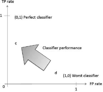
ROC-space with two classifiers c and d. The arrow indicates the direction of overall improvement of classifiers.
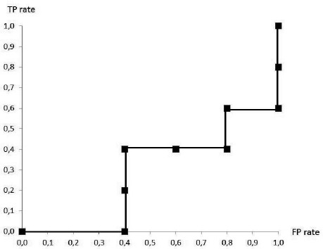
Probabilistic classifiers need a threshold to make a final decision for each class. For each possible threshold, a different discrete classifier is obtained, with a different TP rate and FP rate. By considering all possible thresholds, putting their corresponding classifiers in the ROC space, and drawing a line through them, a so-called ROC curve is obtained. In Figure 24.2, an example of such a stepwise function is given. In this simple example, the curve is constructed by considering all probabilities as thresholds, calculating the corresponding TP rate and FP rate and putting them in the plot. However, when a large dataset needs to be evaluated, more efficient algorithms are required. In that case, Algorithm 24.1 can be used, which only requires O(nlogn) operations. It makes use of the observation that instances classified positive for a certain threshold will also be classified for all lower thresholds. The algorithm sorts the instances decreasing with reference to the outputs p(x) of the classifier, and processes each instance at the time to calculate the corresponding TP rate and FP rate.
Algorithm 24.1 Efficient generation of ROC-curve points.
INPUT: n instances X = {x1,…,xn} estimated probabilities returned by the classifier
{p(x1),…, p(xn)} , true classes {r(x1), …,r(xn }, number of positive instances nP and number of negative instances nN.
Xsorted ← X sorted decreasing by p(x) scores
FP ← 0, TP ← 0
R = 〈〉
pprev ← -221E;
i ← 1
while i ≤|Xsorted| do
if p(xi) ≠ pprev then
push (FP/nN, TP/nP) onto R
pprev ← pxi
end if
if r(Xsorted [i])= P then
TP ← TP+ 1
else
FP ← FP+ 1
end if
i ← i + 1
end while
push (1, 1) onto R
OUTPUT: R, ROC points by increasing FP rate.
ROC curves are a great tool to visualize and analyze the performance of classifiers. The most important advantage is that they are independent of the class distribution, which makes them interesting to evaluate unbalanced problems. In order to compare two probabilistic classifiers with each other, the two ROC curves can be plotted on the same ROC space, as illustrated in Figure 24.3. On the left-hand-side, it is easy to see that classifier A outperforms B , as its ROC-curve is north-west of the ROC-curve of B. This means that for each threshold, the TP rate of A is higher than the TP rate of B, and that the FP rate of B is higher for each threshold. On the right-hand-side, the situation is less obvious and it is hard to say if C is better than D or the other way around. However, some interesting information can be extracted from the graph, that is, we can conclude that C is more precise than D for high thresholds, which means that it is the best choice if not many false positives are allowed. D on the other hand is more appropriate when a high sensitivity is required.
Although this visualization is a handy tool that is frequently used, many researchers prefer a single value to assess the performance of a classifier. The Area-Under the Curve (AUC) is a measure that is often used to that goal. It is the surface between the ROC curve and the horizontal axis, and is a good measure to reflect the quality, as ROC curves that are more to the north west are better and have a bigger surface. AUC values are often used as a single evaluation metric in imbalanced classification problems. In real-world problems, however, one should keep in mind that ROC curves reveal much more information than the single AUC value.
An important point when evaluating classifiers using ROC curves is that they do not measure the absolute performance of the classifier but the relative ranking of the probabilities. For instance, when the probabilities of a classifier are all higher than 0.5 and the threshold is also 0.5, no instance will be classified as negative. However, when all probabilities of the positive instances are higher than the probabilities of the negative instances, the classifier will have a perfect ROC curve and the AUC will be 1. This example shows that determining an appropriate threshold for the final classifier should be done appropriately.
When evaluating probabilistic classifiers for multi-class problems [38], a straightforward option is to decompose the multi-class problems to multiple two-class problems and to carry out the ROC analysis for each two-class problem. Understanding and interpreting these multiple visualizations is challenging, therefore specific techniques for multi-class ROC analysis were developed.
The first approach is discussed in [41], where ROC analysis is extended for three-class classification problems. Instead of an ROC curve, an ROC surface is plotted, and the Volume Under the Surface (VUS) is calculated analogously to the AUC. ROC surfaces can be used to compare classifiers on three-class classification problems by analyzing the maximum information gain on each of them.
ROC analysis for multi-class problems gains more and more attention. In [10], the multi-class problem is decomposed in partial two-class problems, where each problem retains labels of the instances in one specific class, and the instances in the remaining classes get another label. The AUC’s are calculated for each partial problem and the final AUC is obtained by computing the weighted average of the AUC’s, where the weight is determined based on the frequency of the corresponding class in the data. Another generalization is given in [19], where the AUC’s of all combinations of two different classes are computed, and the sum of these intermediate AUCs is divided by the number of all possible misclassifications. The advantage of this approach over the previous one is that this approach is less sensitive to class distributions. In [14], the extension from ROC curve to ROC surface is further extended to ROC hyperpolyhedrons, which are multi-dimensional geometric objects. The volume of these geometric objects is the analogue of the VUS or AUC. A more recent approach can be found in [20], where a graphical visualization of the performance is developed.
To conclude, we note that computational cost is an important issue for multi-class ROC analysis; mostly all pairs of classes need to be considered. Many researchers [31–34] are working on faster approaches to circumvent this problem.
24.3.2 Additional Measures
When evaluating a classifier, one should not only take into account accuracy related measures but also look into other aspects of the classifier. One very important feature of classifiers is time complexity. There are two time measurements. The first one is the time needed to build the model on the training data, the second measures the time needed to classify the test instances based on this model. For some applications it is very important that the time to classify an instance is negligible and meanwhile building the model can be done offline and can take longer. Running time is extremely important when working with big data.
Time complexity can be measured theoretically, but it is good to have an additional practical evaluation of time complexity, where the time is measured during the training and testing phases.
Another important measure is storage requirements of the model. Of course, the initial model is built on the entire data, but after this training phase, the model can be stored elsewhere and the data points are no longer needed. For instance, when using a classification tree, only the tree itself needs to be stored. On the other hand, when using K Nearest Neighbors, the entire dataset needs to be stored and storage requirements are high.
When using active learning algorithms, an additional metric that measures the number of required labels in the train data is needed. This measure is correlated with the time needed to build the model.
24.4 Comparing Classifiers
When evaluating a new classifier, it is important to compare it to the state of the art. Deciding if your new algorithm is better than existing ones is not a trivial task. On average, your algorithm might be better than others. However, it may also happen that your new algorithm is only better for some examples. In general, there is no algorithm that is the best in all situations, as suggested by the no free lunch theorem [53].
For these and other reasons, it is crucial to use appropriate statistical tests to verify that your new classifier is indeed outperforming the state of the art. In this section, we give an overview of the most important statistical tests that can be used and summarize existing guidelines to help researchers to compare classifiers correctly.
A major distinction between different statistical tests is whether they are parametric [48] or non-parametric [5, 18, 37, 48]. All considered statistical tests, both parametric and non-parametric, assume independent instances. Parametric tests, in contrast to non-parametric tests, are based on an underlying parametric distribution of the (transformed) results of the considered evaluation measure. In order to use parametric statistical tests meaningfully, these distributional assumptions on the observations must be fulfilled. In most comparisons, not all these assumptions for parametric statistical tests are fulfilled or too few instances are available to check the validity of these assumptions. In those cases, it is recommended to use non-parametric statistical tests, which only require independent observations. Non-parametric statistical tests can also be used for data that do fulfill the conditions for parametric statistical tests, but it is important to note that in that case, the non-parametric tests have in general lower power than the parametric tests. Therefore, it is worthwhile to first check if the assumptions for parametric statistical tests are reasonable before carrying out any statistical test.
Depending on the setting, pairwise or multiple comparison tests should be performed. A pair-wise test aims to detect a significant difference between two classifiers, while a multiple comparison test aims to detect significant differences between multiple classifiers. We consider two types of multiple comparison tests; in situations where one classifier needs to be compared against all other classifiers, we speak about a multiple comparison test with a control method. In the other case, we want to compare all classifiers with all others and hence we want to detect all pairwise differences between classifiers.
All statistical tests, both parametric and non-parametric, follow the same pattern. They assume a null hypothesis, stating that there is no difference between the classifiers’ performance, e.g., expressed by the mean or median difference in performance. Before the test is carried out, a significance level is fixed, which is an upper bound for the probability of falsely rejecting the null hypothesis. The statistical test can reject the null-hypothesis at this significance level, which means that with high confidence at least one of the classifiers significantly outperforms the others, or not reject it at this significance level, which means that there is no strong or sufficient evidence to believe that one classifier is better than the others. In the latter case, it is not guarenteed that there are no differences between the classifiers; the only conclusion then is that the test cannot find significant differences at this significance level. This might be because there are indeed no differences in performance, or because the power (the probability of correctly rejecting the null hypothesis) of the test is too low, caused by an insufficient amount of datasets. The decision to reject the null hypothesis is based on whether the observed test statistic is bigger than some critical value, or equivalently, whether the corresponding p-value is smaller than the prespecified significance level. Recall that the p-value returned by a statistical test is the probability that a more extreme observation than the observed one, given the null hypothesis, is true.
In the remainder of this section, the number of classifiers is denoted by k, the number of cases (also referred to as instances, datasets, or examples) by n, and the significance level by α. The calculated evaluation measure of case i based on classifier j is denoted Yij.
24.4.1 Parametric Statistical Comparisons
In this section, we first consider a parametric test for a pairwise comparison and next consider a multiple comparison procedure with a discussion on different appropriate post-hoc procedures, taking into account the multiple testing issue.
24.4.1.1 Pairwise Comparisons
In parametric statistical testing, the paired t-test is used to compare the performance of two classifiers (k = 2). The null hypothesis is that the mean performance of both classifiers is the same and one aims to detect a difference in means. The null hypothesis will be rejected if the mean performances are sufficiently different from one another. To be more specific, the sample mean of the differences in performance ˉD=Σni=1(Yi2−Yi2)/n
To check whether the normality assumption is plausible, visual tools like histograms and preferably QQ-plots can be used. Alternatively, one can use a normality test. Three popular normality tests, which all aim to detect certain deviations from normality, are (i) the Kolmogorov-Smirnov test, (ii) the Shapiro-Wilk test, and (iii) the D’Agostino-Pearson test [4].
24.4.1.2 Multiple Comparisons
When comparing more than two classifiers (k > 2), the paired t-test can be generalized to the within-subjects ANalysis Of VAriance (ANOVA, [48]) statistical test. The null hypothesis is that the mean performance of all k classifiers is the same and one aims to detect a deviation from this. The null hypothesis will be rejected if the mean performances of at least two classifiers are sufficiently different from one another in the sense that the mean between-classifier variability (sytematic variability) sufficiently exceeds the mean residual variability (error variability). For this purpose, define ˉY..=Σkj=1Σni=1Yij/nk,ˉYi.=Σkj=1Yij/k
F=M SBCM SBC.
If this quantity is sufficiently large, it is likely that there are significant differences between the different classifiers. Assuming the results for the different instances are normally distributed and assuming sphericity (discussed below), the F-ratio follows an F-distribution with k –1 and (n – 1)(k – 1) degrees of freedom. The null hypothesis is rejected if F > Fk−1(n−1)(k−1)– where Fk−1)(n−1)(k−1)α is the 1 - α percentile of an Fk−1(n−1)(k−1)-distribution. The normality assumption can be checked using the same techniques as for the paired t-test. The sphericity condition boils down to equality of variance of all k(k − 1)/2 pairwise differences, which can be inspected using visual plots such as boxplots. A discussion of tests that are employed to evaluate sphericity is beyond the scope of this chapter and we refer to [29].
If the null hypothesis is rejected, the only information provided by the within-subjects ANOVA is that there are significant differences between the classifiers’ performances, but not information is provided about which classifier outperforms another. It is tempting to use multiple pairwise comparisons to get more information. However, this will lead to an accumulation of the Type I error coming from the combination of pairwise comparisons, also referred to as the Family Wise Error Rate (FWER, [42]), which is the probability of making at least one false discovery among the different hypotheses.
In order to make more detailed conclusions after an ANOVA test rejects the null hypothesis, i.e., significant differences are found, post-hoc procedures are needed that correct for multiple testing to avoid inflation of Type I errors. Most of the post-hoc procedures we discuss here are explained for multiple comparisons with a control method and thus we perform k - 1 post-hoc tests. However, the extension to an arbitrary number of post-hoc tests is straightforward.
The most simple procedure is the Bonferroni procedure [11], which uses paired t-tests for the pairwise comparisons but controls the FWER by dividing the significance level by the number of comparisons made, which here corresponds to an adjusted significane level of α/(k - 1). Equiva-lently, one can multiply the obtained p-values by the number of comparisons and compare to the original significance level α. However, the Bonferonni correction is too conservative when many comparisons are performed. Another approach is the Dunn-Sidak [50] correction, which alters the p-values to 1 - (1 - p)1/(k−1).
A more reliable test when interested in all paired comparisons is Tukey’s Honest Significant Difference (HSD) test [2]. This test controls the FWER so it will not exceed α. To be more specific, suppose we are comparing classifier j with l. The Tukey’s HSD test is based on the studentized range statistic
qjl=|ˉY.j−ˉY.l|√M Sres/n.
It corrects for multiple testing by changing the critical value to reject the null hypothesis. Under the assumptions of the within-subjects ANOVA, qjl follows a studentized range distribution with k and (n - 1)(k - 1) degrees of freedom and the null hypothesis that the mean performance of classifier j is the same of classifier l is rejected if qjl > qk((n−1)(k−1)α where qk((n−1)(k−1)α is the 1 - α percentile of a qk(n−1)(k−1)-distribution.
A similar post-hoc procedure is the Newman-Keuls [28] procedure, which is more powerful than Tuckey’s HSD test but does not guarentee the FWER will not exceed the prespecified significance level α. The Newman-Keuls procedure uses a systematic stepwise approach to carry out many comparisons. It first orders the sample means . For notational convenience, suppose the index j labels these ordered sample means in ascending order: 1 < … < k .In the first step, the test verifies if the largest and smallest sample means significantly differ from each other using the test statistic qn1 and uses the critical value qk,(n−1)(k−1)¡α, if these sample means are k steps away from each other. If the null hypothesis is retained, it means that the null hypotheses of all comparisons will be retained. If the null hypothesis is rejected, all comparisons of sample means that are k - 1 steps from one another are performed, and qn2 and qn−1, 1 are compared to the critical value qk−1,(n−1)(k−1),α.In a stepwise manner, the range between the means is lowered, until no null hypotheses are rejected anymore.
A last important post-hoc test is Scheffe’s test [46]. This test also controls the FWER, but now regardless, the number of post-hoc comparisons. It is considered to be very conservative and hence Tuckey’s HSD test may be preferred. The procedure calculates for each comparison of interest the difference between the means of the corresponding classifiers and compares them to the critical value
√(k−1)Fk−1,(n−1)(k−1),α√2MSresn
where Fk−1(n−1)(k−1),α is the 1 - α percentile of an Fk−1(n−1)(k−1)-disttibution. If the difference in sample means exceeds this critical value, the means of the considered classifiers are significantly different.
24.4.2 Non-Parametric Statistical Comparisons
In the previous section, we discussed that the validity of parametric statistical tests heavily depends on the underlying distributional assumptions of the performance of the classifiers on the different datasets. In practice, not all these assumptions are necessarily fulfilled or too few instances are available to check the validity of these assumptions. In those cases, it is recommended to use non-parametric statistical tests, which only require independent observations. Strictly speaking, the null hypothesis of the non-parametric tests presented here state that the distribution of the performance of all classifiers is the same. Different tests then differ in what alternatives they aim to detect.
Analogous to the previous section about parametric statistical tests, we make a distinction between pairwise and multiple comparisons.
24.4.2.1 Pairwise Comparisons
When comparing two classifiers (k = 2), the most commonly used tests are the sign test and the Wilcoxon signed-ranks test.
Since under the null hypothesis the two classifiers’ scores are equivalent, they each win in approximately half of the cases. The sign test [48] will reject the null hypothesis if for instance the proportion that classifier 1 wins is sufficiently different from 0.5. Let n1 denote the number of times classifier 1 beats classifier 2. Under the null hypothesis, n1 follows a binomial distribution with parameters n and 0.5. The null hypothesis will then be rejected if n1 < kl or n1 > ku where kl is the biggest integer satisfying Σkl−1l=0(nl)0.5n≤α/2
An alternative paired test is Wilcoxon signed-ranks test [52]. The Wilcoxon signed-ranks test uses the differences Yi1 - Yi2. Under the null hypothesis, the distribution of these differences is symmetric around the median and hence we must have that the distribution of the positive differences is the same as the distribution of the negative differences. The Wilcoxon signed rank test then aims to detect a deviation from this to reject the null hypothesis. The procedure assigns a rank to each difference according to the absolute value of these differences, where the mean of ranks is assigned to cases with ties. For instance, when the differences are 0.03, 0.06, -0.03, 0.01, -0.04, and 0.2, the respective ranks are 3.5, 6, 3.5, 1, 5, and 2. Next, the ranks of the positive and negative differences are summed separately, in our case R+ = 12.5and R− = 8.5. When few instances are available, to reject the null hypothesis, min(R+,R−) should be less than or equal to a critical value depending on the significance level and the number of instances; see [48] for tables. Example, when α = 0.1, the critical value is 2, meaning that in our case the null hypothesis is not rejected at the 0.1 significance level. When a sufficient number of instances are available, one can rely on the asymptotic approximation of the distribution of R+ or R−. Let T denote either R+ or R−. Under the null hypothesis, they both have the same approximate normal distribution with mean n(n + 1)/4 and variance n(n + 1)(2n + 1) /24. The Wilcoxon signed rank test then rejects the null hypothesis when
|T−n(n+1)/4|√n(n+1)(2n+1)/24>zα/2
where zα/2 is the 1 − α/2 percentile of the standard normal distribution. An important practical aspect that should be kept in mind is that the Wilcoxon test uses the continuous evaluation measures, so one should not round the values to one or two decimals, as this would decrease the power of the test in case of a high number of ties.
24.4.2.2 Multiple Comparisons
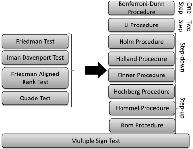
The non-parametric statistical tests that perform multiple comparisons we will discuss in this section are depicted in Figure 24.4. The lower test can be used as a stand-alone method, while the four upper-left tests need a post-hoc procedure to finish the comparison.
Friedman’s test [16, 17] and the Iman Davenport’s test [27] are similar. For each instance, the classifiers are ranked according to the evaluation measure (let rji
χ2=12nk(k+1)(k∑j=1R2j−k(k+1)24).
For a sufficient number of instances and classifiers (as a rule of thumb n > 10 and к > 5), χ2 approximately follows a chi-square distribution with k — 1 degrees of freedom. If χ2 exceeds the critical value χ2k−1,α,
F=(n−1)χ2n(k−1)−χ2
and (assuming a sufficient number of instances and classifiers) follows approximately an F -distribution with k - l and (n- 1)(k - 1) degrees of freedom. If F > Fk-1{n−1)(k−1),α with F(k−1)(n−1)(k−1),α the 1 − α percentile of an Fk−1(n−1)(k−1)-distribution, the null hypothesis is rejected. In both cases, if the test statistic exceeds the corresponding critical value, it means that there are significant differences between the methods, but no other conclusion whatsoever can be made. Next we discuss two more advanced non-parametric tests that in certain circumstances may improve upon the Friedman test, especially when the number of classifiers is low. The Friedman Aligned Rank [22] test calculates the ranks differently. For each data set, the average or median performance of all classifiers on this data set is calculated and this value is substracted from each performance value of the different classifiers to obtain the aligned observations. Next, all kn aligned observations are assigned a rank, the aligned rank Rij with i referring to the data set and j referring to the classifier. The Friedman Aligned Ranks test statistic is given by
T=(k−1)[Σkj=1ˆR2.j−(kn2/4)(kn+1)2][kn(kn+1)(2kn+1)/6]−Σni=1ˆR2i./k
where ˆR⋅j=Σni=1Rij
The Quade test [43] is an improvement upon the Friedman Aligned Ranks test by incorporating the fact that not all data sets are equally important. That is, some data sets are more difficult to classify than others and methods that are able to classify these difficult data sets correctly should be favored. The Quade test computes weighted ranks based on the range of the performances of different classifiers on each data set. To be specific, first calculate the ranks rji
T3=(n−1)Σkj=1S2.j/nn(n+1)(2n+1)k(k+1)(k−1)/72−Σkj=1S2j=1/n
where Sj=Σni=1Sij
When the null hypothesis (stating that all classifiers perform equivalently) is rejected, the average ranks calculated by these four methods themselves can be used to get a meaningful ranking of which methods perform best. However, as was the case for parametric multiple comparisons, post-hoc procedures are still needed to evaluate which pairwise differences are significant. The test statistic to compare algorithm j with algorithm l for the Friedman test and the Iman Davenport’s test is given by
Zjl=Rj−Rl√k(k+1)/6n
with Rj and Rl the average ranks computed in the Friedman and Imand Davenport procedures. For the Friedman Aligned Ranks procedure, the test statistic to compare algorithm j with algorithm l is given by
Zjl=ˆRj−ˆRl√k(k+1)/6
with ˆRj=ˆR⋅j/n
Zjl=Tj−Tl√[k(k+1)(2n+1)(k−1)]/[18n(n+1)]
with Tj=Σni=1Qirji/[n(n+1)/2]
A post-hoc procedure involves multiple pairwise comparisons based on the test statistics Zjl, and as already mentioned for parametric multiple comparisons, these post-hoc tests cannot be used without caution as the FWER is not controlled, leading to inflated Type I errors. Therefore we consider post-hoc procedures based on adjusted p-values of the pairwise comparisons to control the FWER. Recall that the p-value returned by a statistical test is the probability that a more extreme observation than the current one is observed, assuming the null hypothesis holds. This simple p-value reflects this probability of one comparison, but does not take into account the remaining comparisons. Adjusted p-values (APV) deal with this problem and after the adjustment, these APVs can be compared with the nominal significance level α. The post-hoc procedures that we discuss first are all designed for multiple comparisons with a control method, that is, we compare one algorithm against the k - 1 remaining ones. In the following, pj denotes the p-value obtained for the jth null hypothesis, stating that the control method and the jth method are performing equally well. The p-values are ordered from smallest to largest: p1 ≤ … ≤ pk−1, and the corresponding null hypotheses are rewritten accordingly as H1, … ,Hk−1. Below we discuss several procedures to obtain adjusted p-values: one-step, two-step, step-down, and step-up.
1: One-step. The Bonferroni-Dunn [11] procedure is a simple one-step procedure that divides the nominal significance level α by the number of comparisons (k - 1) and the usual p-values can be compared with this level of significance. Equivalently, the adjusted value in this case is min{(k -1)pi, 1}. Although simple, this procedure may be too conservative for practical use when k is not small.
2: Two-step. The two-step Li [36] procedure rejects all null hypotheses if the biggest p-value pk−1 ≤ α. Otherwise, the null hypothesis related to pk−1 is accepted and the remaining null hypotheses Hi with pi ≤ (1 - pk−1)/(1 — α)α are rejected. The adjusted p-values are pi/(pi + 1 - pk−1).
3: Step-down. We discuss three more advanced step-down methods. The Holm [24] procedure is the most popular one and starts with the lowest p-value. If p1 ≤ α/k - 1), the first null hypothesis is rejected and the next comparison is made. If p2 ≤ α/k - 2), the second null hypothesis H2 is also rejected and the next null hypothesis is verified. This process continues until a null hypothesis cannot be rejected anymore. In that case, all remaining null hypotheses are retained as well. The adjusted p-values for the Holm procedure are min [max{(k - j)pj :1 ≤ j ≤ i}, 1]. Next, the Holland [23] procedure is similar to the Holm procedure. It rejects all null hypotheses H1 tot Hi-1 if i is the smallest integer such that pi > 1 - (1 - α)k-i, the adjusted p-values are min[max{1 - (1 -pj)k-j :1 ≤ j ≤ i}, 1]. Finally, the Finner [15] procedure, also similar, rejects all null hypotheses H1 to Hi-1 if i is the smallest integer such that pi > 1 - (1 - α)(k−1/i. The adjusted p-values are min [max{1 - (1 -pj)(k−1)/i :1 ≤ j ≤ i}, 1.]
4: Step-up. Step-up procedures include the Hochberg [21] procedure, which starts off with comparing the largest p-value pk−1 with α, then the second largest p-value pk-2 is compared to α/2 and so on, until a null hypothesis that can be rejected is found. The adjusted p-values are max{(k - j)pj : (k - 1 ) > j > i}. Another more involved procedure is the Hommel [25] procedure. First, it finds the largest j for which pn-j+l > lα/ j for all I = 1,… j. If no such j exists, all null hypotheses are rejected. Otherwise, the null hypotheses for which pi ≤ α/ j are rejected. In contrast to the other procedures, calculating the adjusted p-values cannot be done using a simple formula. Instead the procedure listed in Algorithm 24.2 should be used. Finally, Rom’s [45] procedure was developed to increase Hochberg’s power. It is completely equivalent, except that the α values are now calculated as
αk−i=∑i−1j=1αj∑i−2j=1(ik)αi−jk−1−ji
with αk−1 = α and αk-2 = α/2. Adjusted p-values could also be obtained using the formula for αk-i but no closed form formula is available [18].
Algorithm 24.2 Calculation of the adjusted p-values using Hommels post-hoc procedure.
INPUT: p-values p1 ≤ p2 ≤ pk−1
for all i = 1… k - 1: APVi ←; pi do
for all j = k - 1,k - 2, …, 2 do
B ← ϴ
for all i = k - 1 ,…,k - jdo
ci ← jpi/(j + i - k + 1)
B ← B ⋃ ci
end for
cmin ← min{B}
if APVi < cmin then
APVi ← cmin
end if
for alli = 2,…k- 1 - jdo
ci ← min{cmin, jpi}
if APVi < ci then
APVi ← ci
end if
end for
end for
end for
OUTPUT: Adjusted p-values APV1, …,APVk−1
In some cases, researchers are interested in all pairwisedifferences ina multiple comparison and do not simply want to find significant differences with one control method. Some of the procedures above can be easily extended to this case.
The Nemenyi procedure, which can be seen as a Bonferonni correction, adjusts a in one single step by dividing it by the number of comparisons performed (k( k- 1)/2).
A more involved method is Shaffer’s procedure [47], which is based on the observation that the hypotheses are interrelated. For instance, if method 1 is significantly better than method 2 and method 2 is significantly better than method 3, method 1 will be significantly better than method 3. Shaffer’s method follows a step-down method, and at step j, it rejects Hj if pj ≤ α/tj,where tj is the maximum number of hypotheses that can be true given that hypotheses H1, …Hj-1 are false. This value ti can be found in the table in [47].
Finally, the Bergmann-Hommel [26] procedure says that an index set I ⊆{1,…M}, with M the number of hypotheses, is exhaustive if and only if it is possible that all null hypotheses Hj, j ∈ I could be true and all hypotheses Hj, j φ I are not. Next, the set A is defined as ⋃{I : I exhaustive, min(pi : i ∈ I) > α/|I|, and the procedure rejects all the Hj with j ∈ A.
We now discuss one test that can be used for multiple comparisons with a control algorithm without a further post-hoc analysis needed, the multiple sign test [44], which is an extension of the standard sign test. The multiple sign test proceeds as follows: it counts for each classifier the number of times it outperforms the control classifier and the number of times it is outperformed by the control classifier. Let Rj be the minimum of those two values for the jth classifier. The null hypothesis is now different from the previous ones since it involves median performances. The null hypothesis states that the median performances are the same and is rejected if Rj exceeds a critical value depending on the the nominal significance level α, the number of instances n, and the number k - 1 of alternative classifiers. These critical values can be found in the tables in [44].
All previous methods are based on hypotheses and the only information that can be obtained is if algorithms are significantly better or worse than others. Contrast estimation based on medians [9] is a method that can quantify these differences and reflects the magnitudes of the differences between the classifiers for each data set. It can be used after significant differences are found. For each pair of classifiers, the differences between them are calculated for all problems. For each pair, the median of these differences over all data sets are taken. These medians can now be used to make comparisons between the different methods, but if one wants to know how a control method performs compared to all other methods, the mean of all medians can be taken.
24.4.2.3 Permutation Tests
Most of the previous tests assume that there are sufficient data sets to posit that the test statistics approximately follow a certain distribution. For example, when sufficient data sets are available, the Wilcoxon signed rank test statistic approximately follows a normal distribution. If only a few data sets are available for testing certain algorithms, permutation tests [12], also known as exact tests, are a good alternative to detect differences between classifiers. The idea is quite simple. Under the null hypothesis it is assumed that the distribution of the performance of all algorithms is the same. Hence, the results of a certain classifier j could equally likely be produced by classifier l. Thus, under the null hypothesis, it is equally likely that these results are interchanged. Therefore, one may construct the exact distribution of the considered test statistic by calculating the test statistic under each permutation of the classifier labels within each data set. One can then calculate a p-value as the number of permuted test statistic values that are more extreme than the observed test statistic value devided by the number of random permutations performed. The null hypothesis is rejected when the p-value is smaller than the significance level α. A major drawback of this method is that it is computationally expensive, so it can only be used in experimental settings with few datasets.
In the case where we want to perform multiple comparisons, however, permutation tests give a very elegant way to control the FWER at the prespecified α. Suppose for simplicity we want to perform all pairwise comparisons. For this purpose, we can use the test statistics Zjl defined above in the following manner. Recall that the FWER equals the probabilty of falsely rejecting at least one null hypothesis. Thus, if we find a constant c such that
P(maxj,l|Zjl|>c|H0)=α
and use this constant c as the critical value to reject a certain null hypothesis, we automatically control for the FWER at the α level. To be more specific, we reject those null hypotheses stating that classifier j performs equally well as classifier l if the corresponding observed value for Zjl| exceeds c. This constant can be easily found by taking the 1 - α percentile of the permutation null distribution of maxj,l |Zjl.|
24.5 Concluding Remarks
To conclude, we summarize the considerations and recommendations as listed in [5] for non-parametric statistical tests. First of all, non-parametric statistical tests should only be used given that the conditions for parametric tests are not true. For pairwise comparisons, Wilcoxon’s test is preferred over the sign test. For multiple comparisons, first it should be checked if there are significant differences between the methods, using either Friedman’s (aligned rank) test, Quade’s test or Iman Davenport’s test. The difference in power among these methods is unknown, although it is recommended to use Friedman’s algigned rank test or Quade’s test when the number of algorithms to be compared is rather high. Holm’s post hoc procedure is considered to be one of the best tests. Hochberg’s test has more power and can be used in combination with Holm’s procedure. The multiple sign test is recommended when the differences between the control method and the others are very clear. We add that if only a few datasets are available, permutation tests might be a good alternative.
Bibliography
[1] A. Ben-David. Comparison of classification accuracy using Cohen’s weighted kappa. Expert Systems with Applications, 34(2):825–832, 2008.
[2] A. M. Brown. A new software for carrying out one-way ANOVA post hoc tests. Computer Methods and Programs in Biomedicine, 79(1):89–95, 2005.
[3] A. Celisse and S. Robin. Nonparametric density estimation by exact leave-out cross-validation. Computational Statistics and Data Analysis, 52(5):2350–2368, 2008.
[4] W. W. Daniel. Applied nonparametric statistics, 2nd ed. Boston: PWS-Kent Publishing Company, 1990.
[5] J. Derrac, S. García, D. Molina, and F. Herrera. A practical tutorial on the use of nonpara-metric statistical tests as a methodology for comparing evolutionary and swarm intelligence algorithms. Swarm and Evolutionary Computation, 1(1):3–18, 2011.
[6] L. Devroye and T. Wagner. Distribution-free performance bounds for potention function rules. IEEE Transactions in Information Theory, 25(5):601–604, 1979.
[7] N. A. Diamantidis, D. Karlis, and E. A. Giakoumakis. Unsupervised stratification of cross-validation for accuracy estimation. Artificial Intelligence, 116(1–2): 1–16, 2000.
[8] T. Dietterich. Approximate statistical tests for comparing supervised classification learning algorithms. Neural Computation, 10:1895–1923, 1998.
[9] K. Doksum. Robust procedures for some linear models with one observation per cell. Annals of Mathematical Statistics, 38:878–883, 1967.
[10] P. Domingos and F. Provost. Well-trained PETs: Improving probability estimation trees, 2000. CDER Working Paper, Stern School of Business, New York University, NY, 2000.
[11] O. Dunn. Multiple comparisons among means. Journal of the American Statistical Association, 56:52–64, 1961.
[12] E. S. Edgington. Randomization tests, 3rd ed. New York: Marcel-Dekker, 1995.
[13] B. Efron and R. Tibshirani. Improvements on cross-validation: The .632+ bootstrap method. Journal of the American Statistical Association, 92(438):548–560, 1997.
[14] C. Ferri, J. Hernández-Orallo, and M.A. Salido. Volume under the ROC surface for multi-class problems. In Proc. of 14th European Conference on Machine Learning, pages 108–120, 2003.
[15] H. Finner. On a monotonicity problem in step-down multiple test procedures. Journal of the American Statistical Association, 88:920–923, 1993.
[16] M. Friedman. The use of ranks to avoid the assumption of normality implicit in the analysis of variance. Journal of the American Statistical Association, 32:674–701, 1937.
[17] M. Friedman. A comparison of alternative tests of significance for the problem of m rankings. Annals of Mathematical Statistics, 11:86–92, 1940.
[18] S. García, A. Fernández, J. Luengo, and F. Herrera. Advanced nonparametric tests for multiple comparisons in the design of experiments in computational intelligence and data mining: Experimental analysis of power. Information Sciences, 180:2044–2064, 2010.
[19] D. J. Hand and R. J. Till. A simple generalisation of the area under the ROC curve for multiple class classification problems. Machine Learning, 45(2):171–186, 2001.
[20] M. R. Hassan, K. Ramamohanarao, C. Karmakar, M. M. Hossain, and J. Bailey. A novel scalable multi-class roc for effective visualization and computation. In Advances in Knowledge Discovery and Data Mining, volume 6118, pages 107–120. Springer Berlin Heidelberg, 2010.
[21] Y. Hochberg. A sharper Bonferroni procedure for multiple tests of significance. Biometrika, 75:800–803, 1988.
[22] J. Hodges and E. Lehmann. Ranks methods for combination of independent experiments in analysis of variance. Annals of Mathematical Statistics, 3:482–497, 1962.
[23] M. C. B. S. Holland. An improved sequentially rejective Bonferroni test procedure. Biometrics, 43:417–423, 1987.
[24] S. Holm. A simple sequentially rejective multiple test procedure. Scandinavian Journal of Statistics, 6:65–70, 1979.
[25] G. Hommel. A stagewise rejective multiple test procedure based on a modified Bonferroni test. Biometrika, 75:383–386, 1988.
[26] G. Hommel and G. Bernhard. A rapid algorithm and a computer program for multiple test procedures using logical structures of hypotheses. Computer Methods and Programs in Biomedicine, 43(3–4):213–216, 1994.
[27] R. Iman and J. Davenport. Approximations of the critical region of the Friedman statistic. Communications in Statistics, 9:571–595, 1980.
[28] M. Keuls. The use of the studentized range in connection with an analysis of variance. Euphytica, 1:112–122, 1952.
[29] R. E. Kirk. Experimental design: Procedures for the Behavioral Sciences, 3rd ed. Pacific Grove, CA: Brooks/Cole Publishing Company, 1995.
[30] R. Kohavi. A study of cross-validation and bootstrap for accuracy estimation and model selection. In Proceedings of the 14th International Joint Conference on Artificial Intelligence— Volume 2, IJCAI’95, pages 1137–1143, 1995.
[31] T. C. W. Landgrebe and R. P. W. Duin. A simplified extension of the area under the ROC to the multiclass domain. In 17th Annual Symposium of the Pattern Recognition Association of South Africa, 2006.
[32] T. C. W. Landgrebe and R. P. W. Duin. Approximating the multiclass ROC by pairwise analysis. Pattern Recognition Letters, 28(13):1747–1758, 2007.
[33] T. C. W. Landgrebe and R. P. W. Duin. Efficient multiclass ROC approximation by decomposition via confusion matrix perturbation analysis. IEEE Transactions on Pattern Analysis and Machine Intelligence, 30(5):810–822, 2008.
[34] T. C. W. Landgrebe and P. Paclik. The ROC skeleton for multiclass ROC estimation. Pattern Recognition Letters, 31(9):949–958, 2010.
[35] S. C. Larson. The shrinkage of the coefficient of multiple correlation. Journal of Educational Psychology, 22(1):45–55, 1931.
[36] J. Li. A two-step rejection procedure for testing multiple hypotheses. Journal of Statistical Planning and Inference, 138:1521–1527, 2008.
[37] J. Luengo, S. García, and F. Herrera. A study on the use of statistical tests for experimentation with neural networks: Analysis of parametric test conditions and non-parametric tests. Expert Systems with Applications, 36:7798–7808, 2009.
[38] M. Majnik and Z. Bosnić. ROC analysis of classifiers in machine learning: A survey. Intelligent Data Analysis, 17(3):531–558, 2011.
[39] J. G. Moreno-Torres, T. Raeder, R. A. Rodriguez, N. V. Chawla, and F. Herrera. A unifying view on dataset shift in classification. Pattern Recognition, 45(1):521–530, 2012.
[40] J. G. Moreno-Torres, J. A. Sáez, and F. Herrera. Study on the impact of partition-induced dataset shift on k -fold cross-validation. IEEE Transactions on Neural Networks and Learning Systems, 23(8):1304–1312, 2012.
[41] D. Mossman. Three-way ROCS. Medical Decision Making, 19:78–89, 1999.
[42] T. Nichols and S. Hayasaka. Controlling the familywise error rate in functional neuroimaging: A comparative review. Statistical Methods in Medical Research, 12:419–446, 2003.
[43] D. Quade. Using weighted rankings in the analysis of complete blocks with additive block effects. Journal of the American Statistical Association, 74:680–683, 1979.
[44] A. Rhyne and R. Steel. Tables for a treatments versus control multiple comparisons sign test. Technometrics, 7:293–306, 1965.
[45] D. Rom. A sequentially rejective test procedure based on a modified Bonferroni inequality. Biometrika, 77:663–665, 1990.
[46] H. Scheffé. A method for judging all contrasts in the analysis of variance. Biometrika, 40:87–104, 1953.
[47] J. Shaffer. Modified sequentially rejective multiple test procedures. Journal of American Statistical Association, 81:826–831, 1986.
[48] D. J. Sheskin. Handbook of Parametric and Nonparametric Statistical Procedures, 4th ed., Boca Raton, FL: Chapman and Hall/CRC, 2006.
[49] H. Shimodaira. Improving predictive inference under covariate shift by weighting the log-likelihood function. Journal of Statistical Planning and Inference, 90(2):227–244, 2000.
[50] Z. Sidak. Rectangular confidence regions for the means of multivariate normal distributions. Journal of the American Statistical Association, 62(318):626–633, 1967.
[51] M. Stone. Cross-validatory choice and assessment of statistical predictions. Journal of the Royal Statistics Society, 36:111–147, 1974.
[52] F. Wilcoxon. Individual comparisons by ranking methods. Biometrics Bulletin, 6:80–83, 1945.
[53] D. H. Wolpert. The supervised learning no-free-lunch theorems. In Proceedings of the Sixth Online World Conference on Soft Computing in Industrial Applications, 2001.
[54] Q. S. Xu and Y. Z. Liang. Monte Carlo cross validation. Chemometrics and Intelligent Laboratory Systems, 56(1):1–11, 2001.
[55] J. H. Zar. Biostatistical Analysis. Prentice Hall, 1999.
[56] X. Zeng and T. R. Martinez. Distribution-balanced stratified cross-validation for accuracy estimation. Journal of Experimental and Theoretical Artificial Intelligence, 12(1): 1–12, 2000.