
Collective Classification of Network Data
Ben London
University of Maryland
College Park, MD 20742
[email protected]
Lise Getoor
University of Maryland
College Park, MD 20742
getoor@;cs.umd.edu
15.1 Introduction
Network data has become ubiquitous. Communication networks, social networks, and the World Wide Web are becoming increasingly important to our day-to-day life. Moreover, networks can be defined implicitly by certain structured data sources, such as images and text. We are often interested in inferring hidden attributes (i.e., labels) about network data, such as whether a Facebook user will adopt a product, or whether a pixel in an image is part of the foreground, background, or some specific object. Intuitively, the network should help guide this process. For instance, observations and inference about someone’s Facebook friends should play a role in determining their adoption probability. This type of joint reasoning about label correlations in network data is often referred to as collective classification.
Classic machine learning literature tends to study the supervised setting, in which a classifier is learned from a fully-labeled training set; classification performance is measured by some form of statistical accuracy, which is typically estimated from a held-out test set. It is commonly assumed that data points (i.e., feature-label pairs) are generated independently and identically from an underlying distribution over the domain, as illustrated in Figure 15.1(a). As a result, classification is performed independently on each object, without taking into account any underlying network between the objects. Classification of network data does not fit well into this setting. Domains such as Webpages, citation networks, and social networks have naturally occurring relationships between objects. Because of these connections (illustrated in Figure 15.1(b)), their features and labels are likely to be correlated. Neighboring points may be more likely to share the same label (a phenomenon sometimes referred to as social influence or contagion), or links may be more likely between instances of the same class (referred to as homophily or assortativity). Models that classify each object independently are ignoring a wealth of information, and may not perform well.
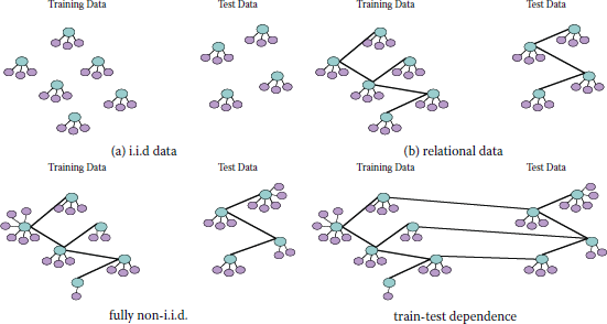
(a) An illustration of the common i.i.d. supervised learning setting. Here each instance is represented by a subgraph consisting of a label node (blue) and several local feature nodes (purple). (b) The same problem, cast in the relational setting, with links connecting instances in the training and testing sets, respectively. The instances are no longer independent. (c) A relational learning problem in which each node has a varying number of local features and relationships, implying that the nodes are neither independent nor identically distributed. (d) The same problem, with relationships (links) between the training and test set.
Classifying real network data is further complicated by heterogenous networks, in which nodes may not have uniform local features and degrees (as illustrated in Figure 15.1(c)). Because of this, we cannot assume that nodes are identically distributed. Also, it is likely that there is not a clean split between the training and test sets (as shown in Figure 15.1(d)), which is common in relational datasets. Without independence between training and testing, it may be difficult to isolate training accuracy from testing accuracy, so the statistical properties of the estimated model are not straightforward.
In this article, we provide an overview of existing approaches to collective classification. We begin by formally defining the problem. We then examine several approaches to collective classification: iterative wrappers for local predictors, graph-based regularization and probabilistic graphical models. To help ground these concepts in practice, we review some common feature engineering techniques for real-world problems. Finally, we conclude with some interesting applications of collective classification.
15.2 Collective Classification Problem Definition
Fix a graph G ≜ (V, E) on n nodes V ≜ {1, … , n}, with edges E ⊆ V × V . For the purposes of this chapter, assume that the structure of the graph is given or implied by an observed network topology. For each node i, we associate two random variables: a set of local features Xi and a label Yi, whose (possibly heterogeneous) domains are Xi and Yi respectively. Assume that the local features of the entire network, X ≜ {X1, … , Xn}, are observed. In some cases, a subset of the labels, Y ≜ {Y1, … , Yn}, are observed as well; we denote the labeled and unlabeled subsets by Yl ⊆ Y and Yu ⊆ Y, respectively, where Yl ⋂ Yu = ∅ and Yl ⋃ Yu = Y. Given X and Yl, the collective classification task is to infer Yu.
In general, collective classification is a combinatorial optimization problem. The objective function varies, depending on the choice of model; generally, one minimizes an energy function that depends on parametric assumptions about the generating distribution. Here we describe several common approaches: iterative classification, label propagation, and graphical models.
Throughout this document, we employ the following notation. Random variables will be denoted by uppercase letters, e.g., X, while realizations of variables will be indicated by lowercase, e.g., x. Sets or vectors of random variables (or realizations) will be denoted by bold, e.g., X (or x). For a node i, let Ni denote the set of indices corresponding to its (open) neighborhood; that is, the set of nodes adjacent to i (but not including it).
15.2.1 Inductive vs. Transductive Learning
Learning scenarios for collective classification broadly fall into two main categories: inductive and transductive. In inductive learning, data is assumed to be drawn from a distribution over the domain; that is, a sentence, image, social network, or some other data structure is generated according to a distribution over instances of said structure. Given a number of labeled structures drawn from this distribution, the objective is to learn to predict on new draws. In the transductive setting, the problem domain is fixed, meaning the data simply exists. The distribution from which the data was drawn is therefore irrelevant, since there is no randomness over what values could occur. Instead, randomness comes from which nodes are labeled, which happens via some stochastic sampling process. Given a labeled subset of the data, the goal is to learn to correctly predict the remaining instances.
In the inductive setting, one commonly assumes that draws of test examples are independent of the training examples. However, this may not hold with relational data, since the data-generating process may inject some dependence between draws from the distribution. There may be dependencies between nodes in the train and test data, as illustrated in Figure 15.1. The same is true of the transductive setting, since the training data may just be a labeled portion of one large network. The dependencies between training and testing must be considered when computing certain metrics, such as train and test accuracy [21].
Since collective methods leverage the correlations between adjacent nodes, researchers typically assume that a small subset of labels are given during prediction. In the transductive setting, these nodes are simply the training set; in the inductive setting, this assumes that draws from the distribution over network structures are partially labeled. However, inductive collective classification is still possible even if no labels are given.
15.2.2 Active Collective Classification
An interesting subproblem in collective classification is how one acquires labels for training (or prediction). In supervised and semi-supervised learning, it is commonly assumed that annotations are given a priori—either adversarially, as in the online model, or agnostically, as in the probably approximately correct (PAC) model. In these settings, the learner has no control over which data points are labeled.
This motivates the study of active learning. In active learning, the learner is given access to an oracle, which it can query for the labels of certain examples. In active collective classification, the learning algorithm is allowed to ask for the labels of certain nodes, so as to maximize its performance using the minimal number of labels. How it decides which labels to query for is an open problem that is generally NP-hard; nonetheless, researchers have proposed many heuristics that work well in practice [4, 21, 27]. These typically involve some trade-off between propagation of information from an acquired label and coverage of the network.
The label acquisition problem is also relevant during inference, since the predictor might have access to a label oracle at test time. This form of active inference has been very successful in collective classification [3, 35]. Queries can sometimes be very sophisticated: a query might return not only a node’s label, but also the labels of its neighbors; if the data graph is uncertain, a query might also return information about a node’s local relationships (e.g., friends, citations, influencers, etc.). This has been referred to as active surveying [30, 38].
Note that an optimal label acquisition strategy for active learning may not be optimal for active inference, so separate strategies may be beneficial. However, the relative performance improvements of active learning and inference are easily conflated, making it difficult to optimize the acquisition strategies. [21] proposes a relational active learning framework to combat this problem.
15.3 Iterative Methods
Collective classification can in some sense be seen as achieving agreement amongst a set of interdependent, local predictions. Viewed as such, some approaches have sought ways to iteratively combine and revise individual node predictions so as to reach an equilibrium. The collective inference algorithm is essentially just a wrapper (or meta-algorithm) for a local prediction subroutine. One of the benefits of this technique is that local predictions can be made efficiently, so the compexity of collective inference is effectively the number of iterations needed for convergence. Though neither convergence nor optimality is guaranteed, in practice, this approach typically converges quickly to a good solution, depending on the graph structure and problem complexity. The methods presented in this section are representative of this iterative approach.
15.3.1 Label Propagation
A natural assumption in network classification is that adjacent nodes are likely to have the same label, (i.e., contagion). If the graph is weighted, then the edge weights {wi,j}(i,j)∈E can be interpreted as the strength of the associativity. Weights can sometimes be derived from observed features X via a similarity function. For example, a radial basis function can be computed between adjacent nodes (i, j) as
wi,j≜exp(||Xi−Xj||22σ2),(15.1)
where σ is a parameter that determines the width of the Gaussian.
Suppose the labels are binary, with Yi ∈ {±1} for all i = 1, …, n. If node i is unlabeled, we could predict a score for Yi = 1(or Yi = −1) as the weighted average of its neighbors’ labels, i.e.,
Yi←(1∑j∈Niwi,j)∑j∈Niwi,jYj.
One could then clamp Yi to {±1} using its sign, sgn(Yi). While we probably will not know all of the labels of Ni, if we already had predictions for them, we could use these, then iterate until the predictions converge. This is precisely the idea behind a method known as label propagation. Though the algorithm was originally proposed by [48] for general transductive learning, it can easily be applied to network data by constraining the similarities according to a graph. An example of this is the modified adsorption algorithm [39].
Algorithm 15.1 provides pseudocode for a simple implementation of label propagation. The algorithm assumes that all labels are k-valued, meaning |Yi| = k for all i = 1, … , n. It begins by constructing a n × k label matrix Y ∈ ℝn×k, where entry i, j corresponds to the probability that Yi = j. The label matrix is initialized as
Yi,j={1if Yi∈Yl and Yi=j,0if Yi∈Yl and Yi≠j,1/kif Yi∈Yu.(15.2)
It also requires an n×n transition matrix T∈ ℝn×n; semantically, this captures the probability that a label propagates from node i to node j, but it is effectively just the normalized edge weight, defined as
Ti,j={wi,j∑j∈Niwi,jif j∈Ni,0if j∉Ni.(15.3)
The algorithm iteratively multiplies Y by T, thereby propagating label probabilities via a weighted average. After the multiply step, the unknown rows of Y, corresponding to the unknown labels, must be normalized, and the known rows must be clamped to their known values. This continues until the values of Y have stabilized (i.e., converged to within some sufficiently small ɛ of change), or until a maximum number of iterations has been reached.
Algorithm 15.1 Label propagation
1: Initialize Y per Equation (15.2)
2: Initialize T per Equation (15.3)
3: repeat
4: Y←TY
5: Normalize unknown rows of Y
6: Clamp known rows of Y using known labels
7: until convergence or maximum iterations reached
8: Assign to Yi the jth label, where j is the highest value in row i of Y.
One interesting property of this formulation of label propagation is that it is guaranteed to converge to a unique solution. In fact, there is a closed-form solution, which we will describe in Section 15.4.
15.3.2 Iterative Classification Algorithms
While label propagation is surprisingly effective, its predictor is essentially just a weighted average of neighboring labels, which may sometimes fail to capture complex relational dynamics. A more sophisticated approach would be to use a richer predictor. Suppose we have a classifier h that has been trained to classify a node i, given its features Xi and the features XNi and labels YNi of its neighbors. Iterative classification does just that, applying local classification to each node, conditioned on the current predictions (or ground truth) on its neighbors, and iterating until the local predictions converge to a global solution. Iterative classification is an “algorithmic framework,” in that it is it is agnostic to the choice of predictor; this makes it a very versatile tool for collective classification.
[6] introduced this approach and reported impressive gains in classification accuracy. [31] further developed the technique, naming it “iterative classification,” and studied the conditions under which it improved classification performance [14]. Researchers [24, 25, 28] have since proposed various improvements and extensions to the basic algorithm we present.
Algorithm 15.2 Iterative classification
1: for Yi ∈ Yu do [Bootstrapping]
2: Yi←h(Xi,XNi,YlNi)Yi←h(Xi,XNi,YlNi)
3: end for
4: repeat [update predicted labels]
5: π ← GENPERM(n) # generate permutation π over 1, … , n
6: for i = 1, … , n do
7: if Yπ(i) ∈ Yu then
8: Yπ(i)←h(Xπ(i), XNπ(i), YNπ(i)))
9: end if
10: end for
11: until convergence or maximum iterations reached
Algorithm 15.2 depicts pseudo-code for a simple iterative classification algorithm. The algorithm begins by initializing all unknown labels Yu using only the features (Xi, XNi). and observed neighbor labels YlNi⊆YNi
Clearly, the order in which nodes are updated affects the predictive accuracy and convergence rate, though there is some evidence to suggest that iterative classification is fairly robust to a number of simple ordering strategies—such as random ordering, ascending order of neighborhood diversity and descending order of prediction confidences [11]. Another practical issue is when to incorporate the predicted labels from the previous round into the the current round of prediction. Some researchers [28, 31] have proposed a “cautious” approach, in which only predicted labels are introduced gradually. More specifically, at each iteration, only the top k most confident predicted labels are used, thus ignoring less confident, potentially noisy predictions. At the start of the algorithm, k is initialized to some small number; then, in subsequent iterations, the value of k is increased, so that in the last iteration all predicted labels are used.
One benefit of iterative classification is that it can be used with any local classifier, making it extremely flexible. Nonetheless, there are some practical challenges to incorporating certain classifiers. For instance, many classifiers are defined on a predetermined number of features, making it difficult to accommodate arbitrarily-sized neighborhoods. A common workaround is to aggregate the neighboring features and labels, such as using the proportion of neighbors with a given label, or the most frequently occurring label. For classifiers that return a vector of scores (or conditional probabilities) instead of a label, one typically uses the label that corresponds to the maximum score. Some of the classifiers used included: naïve Bayes [6, 31], logistic regression [24], decision trees, [14] and weighted-majority [25].
Iterative classification prescribes a method of inference, but it does not instruct how to train the local classifiers. Typically, this is performed using traditional, non-collective training.
15.4 Graph-Based Regularization
When viewed as a transductive learning problem, the goal of collective classification is to complete the labeling of a partially-labeled graph. Since the problem domain is fixed (that is, the data to be classified is known), there is no need to learn an inductive model;1 simply the predictions for the unknown labels will suffice. A broad category of learning algorithms, known as graph-based regularization techniques, are designed for this type of model-free prediction. In this section, we review these methods.
For the remainder of this section, we will employ the following notation. Let y ∈ ℝn denote a vector of labels corresponding to the nodes of the graph. For the methods considered in this section, we assume that the labels are binary; thus, if the ith label is known, then yi ∈ {±1}, and otherwise, yi = 0. The learning objective is to produce a vector h ∈ ℝn of predictions that minimizes the L2 distance to y for the known labels. We can formulate this as a weighted inner product using a diagonal matrix C ∈ ℝn×n, where the (i, i) entry is set to 1 if the ith label is observed and 0 otherwise.2 The error can thus be expressed as
(h−y)⊤C(h−y).
Unconstrained graph-based regularization methods can be generalized using the following abstraction (due to [8]). Let Q ∈ ℝn×n denote a symmetric matrix, whose entries are determined based on the structure of the graph G, the local attributes X (if available), and the observed labels Yl. We will give several explicit definitions for Q shortly; for the time being, it will suffice to think of Q as a regularizer on h. Formulated as an unconstrained optimization, the learning objective is
argminh⊤Qh+h(h−y)⊤C(h−y).
One can interpret the first term as penalizing certain label assignments, based on observed information; the second term is simply the prediction error with respect to the training labels. Using vector calculus, we obtain a closed-form solution to this optimization as
h*=(C−1Q+I)−1y=(Q+C)−1Cy,(15.4)
where I is the n × n identity matrix. This is fairly efficient to compute for moderate-sized networks; the time complexity is dominated by O(n3) operations for the matrix inversion and multiplication. For prediction, the “soft” values of h can be clamped to {±1} using the sign operator.
The effectiveness of this generic approach comes down to how one defines the regularizer, Q. One of the first instances is due to [49]. In this formulation, Q is a graph Laplacian, constructed as follows: for each edge (i, j) ∈ E, define a weight matrix W ∈ ∝n×n, where each element wi,j is defined using the radial basis function in (15.1); define a diagonal matrix D ∈ ℝn×n as
di,i≜n∑j=1wi,j;
one then computes the regularizer as
Q≜D−W.
One could alternately define the regularizer as a normalized Laplacian,
Q≜I−D−12WD−12,
per [47]. [15] extended this method for heterogeneous networks—that is, graphs with multiple types of nodes and edges. Another variant, due to [43], sets
Q≜(I−A)⊤(I−A),
where A ∈ ℝn×n is a row-normalized matrix capturing the local pairwise similarities. All of these formulations impose a smoothness constraint on the predictions, that “similar” nodes—where similarity can be defined by the Gaussian in (15.1) or some other kernel—should be assigned the same label.
There is an interesting connection between graph-based regularization and label propagation. Under the various parameterizations of Q, one can show that (15.4) provides a closed-form solution to the label propagation algorithm in Section 15.3.1 [48]. This means that one can compute certain formulations of label propagation without directly computing the iterative algorithm. Heavily optimized linear algebra solvers can be used to compute (15.4) quickly. Another appealing aspect of these methods is their strong theoretical guarantees [8].
15.5 Probabilistic Graphical Models
Graphical models are powerful tools for joint, probabilistic inference, making them ideal for collective classification. They are characterized by a graphical representation of a probability distribution P, in which random variables are nodes in a graph G. Graphical models can be broadly categorized by whether the underlying graph is directed (e.g., Bayesian networks or collections of local classifiers) or undirected (e.g., Markov random fields). In this section, we discuss both kinds.
Collective classification in graphical models involves finding the assignment yu that maximized the conditional likelihood of Yu, given evidence (X = x, Yl = yl); i.e.,
argmaxyP(Yu=yu|X=x,Yl=yl),(15.5)
where y =(yl, yu). This type of inference—known alternately as maximum a posteriori (MAP) or most likely explanation (MPE)—is known to be NP-hard in general graphical models, though there are certain exceptions in which it can be computed efficiently, and many approximation algorithms that perform well in most settings. We will review selected inference algorithms where applicable.
15.5.1 Directed Models
The fundamental directed graphical model is a Bayesian network (also called Bayes net, or BN).
Definition 15.5.1 (Bayesian Network) A Bayesian network consists of a set of random variables Z ≜ {Z1, … , Zn}, a directed, acyclic graph (DAG) G ≜ (V ,E), and a set of conditional probability distributions (CPDs), {P(Zi|Zpi)}ni=1, where Pi denotes the indices corresponding to the causal parents of Zi. When multiplied, the CPDs describe the joint distribution of Z; i.e., P(Z) = Πi P(Zi |ZPi).
BNs model causal relationships, which are captured by the directionalities of the edges; an edge (i, j) ∈ E indicates that Zi influences Zj. For a more thorough review of BNs, see [18] or Chapter X of this book.
Though BNs are very popular in machine learning and data mining, they can only be used for models with fixed structure, making them inadequate for problems with arbitrary relational structure. Since collective classification is often applied to arbitrary data graphs—such as those found in social and citation networks—some notion of templating is required. In short, templating defines subgraph patterns that are instantiated (or, grounded) by the data graph; model parameters (CPDs) are thus tied across different instantiations. This allows directed graphical models to be used on complex relational structures.
One example of a templated model is probabilistic relational models (PRMs) [9, 12]. A PRM is a directed graphical model defined by a relational database schema. Given an input database, the schema is instantiated by the database records, thus creating a BN. This has been shown to work for some collective classification problems [12, 13], and has the advantage that a full joint distribution is defined.
To satisfy the requirement of acyclicity when the underlying data graph is undirected, one constructs a (templated) BN or PRM as follows. For each potential edge {i, j} in data graph, define a binary random variable Ei,j. Assume that a node’s features are determined by its label. If we further assume that its label is determined by its neighbors’ labels (i.e., contagion), then we draw a directed edge from each Ei, j to the corresponding Yi and Yj, as illustrated in Figure 15.2a. On the other hand, if we believe that a node’s label determines who it connects to (i.e., homophily), then we draw an edge from each Yi to all Ei., as shown in Figure 15.2b. The direction of causality is a modeling decision, which depends on one’s prior belief about the problem. Note that, in both cases, the resulting graphical model is acyclic.
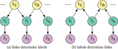
Example BN for collective classification. Label nodes (green) determine features (purple), which are represented by a single vector-valued variable. An edge variable (yellow) is defined for all potential edges in the data graph. In (a), labels are determined by link structure, representing contagion. In (b), links are functions of labels, representing homophily. Both structures are acyclic.
Another class of templated, directed graphical models is relational dependency networks (RDNs) [32]. RDNs have the advantage of supporting graph cycles, though this comes at the cost of consistency; that is, the product of an RDN’s CPDs does not necessarily define a valid probability distribution. RDN inference is therefore only approximate, but can be very fast. Learning RDNs is also fast, because it reduces to independently learning a set of CPDs.
15.5.2 Undirected Models
While directed graphical models are useful for their representation of causality, sometimes we do not need (or want) to explicitly define causality; sometimes we only know the interactions between random variables. This is where undirected graphical models are useful. Moreover, undirected models are strictly more general than directed models; any directed model can be represented by an undirected model, but there are distributions induced by undirected models that cannot be reproduced in directed models. Specifically, graph structures involving cycles are representable in undirected models, but not in directed models.
Most undirected graphical models fall under the umbrella of Markov random fields (MRFs), sometimes called Markov networks [40].
Definition 15.5.2 (Markov random field) A Markov random field (MRF) is defined by a set of random variables Z ≜ {Z1, …, Zn}, a graph G ≜ (V , E), and a set of clique potentials {φc : dom(c)→ℝ}c∈C, where C is a set of predefined cliques and dom(c) is the domain of clique c. (To simplify notation, assume that potential φ;c only operates on the set of variables contained in clique c.) The potentials are often defined as a log-linear combination of features fc and weights wc, such that φc(z) ≜ exp(wc ⋅ fc(z)). An MRF defines a probability distribution P that factorizes as
P(Z=z)=1Φ∏c∈Cϕc(z)=1Φexp(∑c∈Cwc⋅fc(z)),
where Φ≜∑z′∏c∈Cϕc(z′) is a normalizing constant. This model is said to be Markovian because any variable Zi is independent of any non-adjacent variables, conditioned its neighborhood ZNi(sometimes referred to as its Markov blanket).
For collective classification, one can define a conditional MRF (sometimes called a CRF), whose conditional distribution is
P(Yu=yu|X=x,Yl=yl)=1Φ∏c∈Cϕc(x,y)=1Φexp(∑c∈Cwc⋅fc(x,y)).
For relational tasks, such as collective classification, one typically defines the cliques via templating. Similar to a PRM (see Section 15.5.1), a clique template is just a subgraph pattern—although in this case it is a fully-connected, undirected subgraph. The types of templates used directly affects model complexity, in that smaller templates correspond to a simpler model, which usually generalizes better to unseen data. Thus, MRFs are commonly defined using low-order templates, such as singletons, pairs, and sometimes triangles. Examples of templated MRFs include relational MRFs [40], Markov logic networks [36], and hinge-loss Markov random fields [2].
To make this concrete, we consider the class of pairwise MRFs. A pairwise MRF has features and weights for all singleton and pairwise cliques in the graph; thus, its distribution factorizes as
P(Z=z)=1Φ(∏{i,j} ∈ Eϕi,j(z))(∏{i,j} ∈ Eϕi,j(z))=1Φexp[(∑i ∈ Vwi⋅fi(z))+(∑{i,j} ∈ Ewi,j⋅fi,j(z))].
(Since it is straightforward to derive the posterior distribution for collective classification, we omit it here.) If we assume that the domains of the variables are discrete, then it is common to define the features as basis vectors indicating the state of the assignment. For example, if |Zi| = k for all i, then fi(z) is a length-k binary vector, whose jth entry is equal to one if zi is in the jth state and zero otherwise; similarly, fi,j (z) has length k2 and the only nonzero entry corresponds to the joint state of (zi, zj). To make this MRF templated, we simply replace all wi with a single wsingle, and all wi,j with a single wpair.
It is important to note that the data graph does not necessarily correspond to the graph of the MRF; there is some freedom in how one defines the relational features {fi, j}{i, j}∈E. However, when using a pairwise MRF for collective classification, it is natural to define a relational feature for each edge in the data graph. Defining fi,j as a function of (Yi,Yj) models the dependence between labels. One may alternately model (Xi,Yi,Xj,Yj) to capture the pairwise interactions of both features and labels.
15.5.3 Approximate Inference in Graphical Models
Exact inference in general graphical models is intractable, depending primarily on the structure of the underlying graph. Specifically, inference is exponential in the graph’s treewidth. For structures with low treewidth—such as chains and trees—exact inference can be relatively fast. Unfortunately, these tractable settings are rare in collective classification, so inference is usually computed approximately. In this section, we review some commonly used approximate inference algorithms for directed and undirected graphical models.
15.5.3.1 Gibbs Sampling
Gibbs sampling is a general framework for approximating a distribution, when the distribution is presumed to come from a specified family, such as Gaussian, Poisson, etc. It is a Markov chain Monte Carlo (MCMC) algorithm, in that it iteratively samples from the current estimate of the distribution, constructing a Markov chain that converges to the target (stationary) distribution. Gibbs sampling is efficient because it samples from the conditional distributions of the individual variables, instead of the joint distribution over all variables. To make this more concrete, we examine Gibbs sampling for inference in directed graphical models, in the context of collective classification.
Pseudocode for a Gibbs sampling algorithm (based on [10, 25]) is given in Algorithm 15.3. At a high level, the algorithm works by iteratively sampling from the posterior distribution of each Yi, i.e., random draws from P(Yi|X,YNi). Like iterative classification, it initializes the posteriors using some function of the local and neighboring features, as well as any observed neighboring labels; this could be the (normalized) output of a local predictor. It then iteratively samples from each of the current posteriors and uses the sampled values to update the probabilities. This process is repeated until the posteriors converge, or until a maximum number of iterations is reached. Upon terminating, the samples for each node are averaged to obtain the approximate marginal label probabilities, P(Yi = y) (which can be used for prediction by choosing the label with the highest marginal probability). In practice, one typically sets aside a specified number of initial iterations as “burn-in” and averages over the remaining samples. In the limit of infinite data, the estimates should asymptotically converge to the true distribution.
Gibbs sampling is a popular method of approximate (marginal) inference in directed graphical models, such as BNs and PRMs. While each iteration of Gibbs sampling is relatively efficient, many iterations are required to obtain an accurate estimate of the distribution, which may be impractical. Thus, there is a trade-off between the running time and the accuracy of the approximate marginals.
1: for i = 1, … , n do [bootstrapping]
2: Initialize P(Yi|X, YNi) using local features Xi and the features XNi and observed labels YlNi⊆YNi of its neighbors
3: end for
4: for i = 1 , … , n do [initialize samples]
5: Si ← 0
6: end for
7: repeat[sampling]
8: π ← GENPERM (n) # generate permutation π over 1, … , n
9: for i = 1, …, n do
10: Sample s ~ P(Yi |X, YNi)
11: Si ← Si ⋃ s
12: Update P(Yi |X, YNi) using Si
13: end for
14: until convergence or maximum iterations reached
15: for i = 1, … , n do [compute marginals]
16: Remove first T samples (i.e., burn-in) from Si
17: for y ∈ Yi do
18: P(Yi=y)←1|Si|∑s∈Si1[y=s]
19: end for
20: end for
15.5.3.2 Loopy Belief Propagation (LBP)
For certain undirected graphical models, exact inference can be computed efficiently via message passing, or belief propagation (BP), algorithms. These algorithms follow a simple iterative pattern: each variable passes its “beliefs” about its neighbors’ marginal distributions, then uses the incoming messages about its own value to updates its beliefs. Convergence to the true marginals is guaranteed for tree-structured MRFs, but is not guaranteed for MRFs with cycles. That said, BP can still be used for approximate inference in general, so-called “loopy” graphs, with a minor modification: messages are discounted by a constant factor (sometimes referred to as damping). This algorithm is known as loopy belief propagation (LBP).
The LBP algorithm shown in Algorithm 15.4 [45, 46] assumes that the model is a pairwise MRF with singleton potentials defined on each (Xi,Yi) and pairwise potentials on each adjacent (Yi,Yj). We denote by mi→j(y) the message sent by Yi to Yj regarding the belief that Yj = y; ϕi(y) denotes the ith local potential function evaluated for Yi = y, and similarly for the pairwise potentials; α ∈ (0,1] denotes a constant discount factor. The algorithm begins by initializing all messages to one. It then iterates over the message passing pattern, wherein Yi passes its beliefs mi→j(y) to all j ∈ Ni, using the incoming messages mk→j(y) for all j ∈ Ni, from the previous iteration. Similar to Gibbs sampling, the algorithm iterates until the messages stabilize, or until a maximum number of iterations is reached, after which we compute the approximate marginal probabilities.
15.6 Feature Construction
Thus far, we have used rather abstract problem representations, using an arbitrary data graph G ≜ (V ,E), feature variables X, and label variables Y. In practice, how one maps a real-world problem to these representations can have a greater impact than the choice of model or inference algorithm. This process, sometimes referred to as feature construction (or feature engineering), is perhaps the most challenging aspect of data mining. In this section, we explore various techniques, motivated by concrete examples.
Algorithm 15.4 Loopy Belief Propagation
1: for {i, j} ∈ E do [initialize messages]
2: for y ∈ Yj do
3: mi→j (y) ←1
4: end for
5: end for
6: repeat [message passing]
7: for {i, j} ∈ E do
8: for y ∈ Yj do
9: mi→j(y)←α∑y′ϕi,j(y′,y)ϕi(y′)Πk∈Nijmk→i(y′)
10: end for
11: end for
12: until convergence or maximum iterations reached
13: for i = 1, … , n do [compute marginals]
14: for y ∈ Yi do
15: P(Yi=y)←αϕi(y)Πj∈Nimj→i(y)
16: end for
17: end for
15.6.1 Data Graph
Network structure is explicit in certain collective classification problems, such as categorizing users in a social network or pages in a Web site. However, there are other problems that exhibit implicit network structure.
An example of this is image segmentation, a common computer vision problem. Given an observed image—i.e., an m × n matrix of pixel intensities—the goal is to label each pixel as being part of a certain object, from a predetermined set of objects. The structure of the image naturally suggests a grid graph, in which each pixel (i, j) is a node, adjacent to (up to) four neighboring pixels. However, one could also define the neighborhood using the diagonally adjacent pixels, or use wider concentric rings. This decision reflects on one’s prior belief of how many pixels directly interact with (i, j); that is, its Markov blanket.
A related setting is part-of-speech (POS) tagging in natural language processing. This task involves tagging each word in a sentence with a POS label. The linear structure of a sentence is naturally represented by a path graph; i.e., a tree in which each vertex has either one or two neighbors. One could also draw edges between words separated by two hops, or, more generally, n hops, depending on one’s belief about sentence construction.
The data graph can also be inferred from distances. Suppose the task is to predict which individuals in a given population will contract the flu. Infection is obviously related to proximity, so it is natural to construct a network based on geographic location. Distances can be thresholded to create unweighted edges (e.g., “close” or “not close”), or they can be incorporated as weights (if the model supports it).
Structure can sometimes be inferred from other structure. An example of this is found in document classification in citation networks. In a citation network, there are explicit links from papers citing other papers. There are also implicit links between two papers that cite the same paper. These “co-citation” edges complete a triangle between three connected nodes.
Links can also be discovered as part of the inference problem [5, 26]. Indeed, collective classification and link prediction are complimentary tasks, and it has been shown that coupling these predictions can improve overall accuracy [29].
It is important to note that not all data graphs are unimodal—that is, they may involve multiple types of nodes and edges. In citation networks, authors write papers; authors are affiliated with institutions; papers cite other papers; and so on.
15.6.2 Relational Features
Methods based on local classifiers, such as ICA, present a unique challenge to relational feature engineering: while most local classifiers require fixed-length feature vectors, neighborhood sizes are rarely uniform in real relational data. For example, a paper can have any number of authors. If the number of neighbors is bounded by a reasonably small constant (a condition often referred to as bounded degree), then it is possible to represent neighborhood information using a fixed-length vector. However, in naturally occurring graphs, such as social networks, this condition is unlikely.
One solution is to aggregate neighborhood information into a fixed number of statistics. For instance, one could count the number of neighbors exhibiting a certain attribute; for a set of attributes, this amounts to a histogram. For numerical or ordinal attributes, one could also use the mean, mode, minimum or maximum. Another useful statistic is the number of triangles, which reflects the connectivity of the neighborhood. More complex, domain-specific aggregates are also possible. Within the inductive logic programming community, aggregation has been studied as a means for propositionalizing a relational classification problem [17, 19, 20]. In the machine learning community, [33, 34] have studied aggregation extensively.
Aggregation is also useful for defining relational features in graphical models. Suppose one uses a pairwise MRF for social network classification. For each pair of nodes, one could obviously consider the similarities of their local features; yet one could also consider the similarities of their neighborhood structures. A simple metric is the number of common neighbors. To compensate for varying neighborhood sizes, one could normalize the intersection by the union, which is known as Jaccard similarity,
J(Ni,Nj,)≜Ni∩NjNi∪Nj.
This can be generalized to the number (or proportion) of common neighbors who exhibit a certain attribute.
15.7 Applications of Collective Classification
Collective classification is a generic problem formulation that has been successfully applied to many application domains. Over the course of this chapter, we have already discussed a few popular applications, such as document classification [41, 44], image segmentation [1] and POS tagging [22]. In this section, we briefly review some other uses.
One such problem, which is related to POS tagging, is optical character recognition (OCR). The goal of OCR is to automatically convert a digitized stream of handwritten characters into a text file. In this context, each node represents a scanned character; its observed features Xi are a vectorized pixel grid, and the label Yi is chosen from the set of ASCII (or ISO) characters. While this can be predicted fairly well using a local classifier, it has been shown that considering intra-character relationships can be beneficial [42], since certain characters are more (or less) likely to occur before (or after) other characters.
Another interesting application is activity detection in video data. Given a recorded video sequence (say, from a security camera) containing multiple actors, the goal is to label each actor as performing a certain action (from a predefined set of actions). Assuming that bounding boxes and tracking (i.e., identity maintenance) are given, one can bolster local reasoning with spatiotemporal relational reasoning. For instance, it is often the case that certain actions associate with others: if an actor is crossing the street, then other actors in the proximity are likely crossing the street; similarly, if one actor is believed to be talking, then other actors in the proximity are likely either talking or listening. One could also reason about action transitions: if an actor is walking at time t, then it is very likely that they will be walking at time t +1; however, there is a small probability that they may transition to a related action, such as crossing the street or waiting. Incorporating this high-level relational reasoning can be considered a form of collective classification. This approach has been used in a number of publications [7, 16] to achieve current state-of-the-art performance on benchmark datasets.
Collective classification is also used in computational biology. For example, researchers studying protein-protein interaction networks often need to annotate proteins with their biological function. Discovering protein function experimentally is expensive. Yet, protein function is sometimes correlated with interacting proteins; so, given a set of labeled proteins, one can reason about the remaining labels using collective methods [23].
The final application we consider is viral marketing, which is interesting for its relationship to active collective classification. Suppose a company is introducing a new product to a population. Given the social network and the individuals’ (i.e., local) demographic features, the goal is to determine which customers will be interested in the product. The mapping to collective classification is straightforward. The interesting subproblem is in how one acquires labeled training data. Customer surveys can be expensive to conduct, so companies want to acquire the smallest set of user opinions that will enable them to accurately predict the remaining user opinions. This can be viewed as an active learning problem for collective classification [3].
15.8 Conclusion
Given the recent explosion of relational and network data, collective classification is quickly becoming a mainstay of machine learning and data mining. Collective techniques leverage the idea that connected (related) data objects are in some way correlated, performing joint reasoning over a high-dimensional, structured output space. Models and inference algorithms range from simple iterative frameworks to probabilistic graphical models. In this chapter, we have only discussed a few; for greater detail on these methods, and others we did not cover, we refer the reader to [25] and [37]. Many of the algorithms discussed herein have been implemented in NetKit-SRL,3 an open-source toolkit for mining relational data.
Acknowledgements
This material is based on work supported by the National Science Foundation under Grant No. 0746930 and Grant No. IIS1218488.
Bibliography
[1] D. Anguelov, B. Taskar, V. Chatalbashev, D. Koller, D. Gupta, G. Heitz, and A. Ng. Discriminative learning of Markov random fields for segmentation of 3D scan data. In International Conference on Computer Vision and Pattern Recognition, pages 169–176, 2005.
[2] Stephen H. Bach, Bert Huang, Ben London, and Lise Getoor. Hinge-loss Markov random fields: Convex inference for structured prediction. In Uncertainty in Artificial Intelligence, 2013.
[3] Mustafa Bilgic and Lise Getoor. Effective label acquisition for collective classification. In ACM SIGKDD International Conference on Knowledge Discovery and Data Mining, pages 43–51, 2008. Winner of the KDD’08 Best Student Paper Award.
[4] Mustafa Bilgic, Lilyana Mihalkova, and Lise Getoor. Active learning for networked data. In Proceedings of the 27th International Conference on Machine Learning (ICML-10), 2010.
[5] Mustafa Bilgic, Galileo Mark Namata, and Lise Getoor. Combining collective classification and link prediction. In Workshop on Mining Graphs and Complex Structures in International Conference of Data Mining, 2007.
[6] Soumen Chakrabarti, Byron Dom, and Piotr Indyk. Enhanced hypertext categorization using hyperlinks. In International Conference on Management of Data, pages 307–318, 1998.
[7] W. Choi, K. Shahid and S. Savarese. What are they doing?: Collective activity classification using spatio-temporal relationship among people. In VS, 2009.
[8] Corinna Cortes, Mehryar Mohri, Dmitry Pechyony, and Ashish Rastogi. Stability analysis and learning bounds for transductive regression algorithms. CoRR, abs/0904.0814, 2009.
[9] N. Friedman, L. Getoor, D. Koller, and A. Pfeffer. Learning probabilistic relational models. In International Joint Conference on Artificial Intelligence, 1999.
[10] S. Geman and D. Geman. Stochastic relaxation, Gibbs distributions, and the Bayesian restoration of images. Morgan Kaufmann Publishers Inc., San Francisco, CA, 1990.
[11] L. Getoor. Link-based classification. In Advanced Methods for Knowledge Discovery from Complex Data, Springer, 2005.
[12] Lise Getoor, Nir Friedman, Daphne Koller, and Ben Taskar. Learning probabilistic models of link structure. Journal of Machine Learning Research, 3:679–707, 2002.
[13] Lise Getoor, Eran Segal, Benjamin Taskar, and Daphne Koller. Probabilistic models of text and link structure for hypertext classification. In IJCAI Workshop on Text Learning: Beyond Supervision, 2001.
[14] D. Jensen, J. Neville, and B. Gallagher. Why collective inference improves relational classification. In Proceedings of the 10th ACM SIGKDD International Conference on Knowledge Discovery and Data Mining, pages 593–598, 2004.
[15] Ming Ji, Yizhou Sun, Marina Danilevsky, Jiawei Han, and Jing Gao. Graph regularized transductive classification on heterogeneous information networks. In Proceedings of the 2010 European Conference on Machine Learning and Knowledge Discovery in Databases: Part I, ECML PKDD’10, pages 570–586, Berlin, Heidelberg, 2010. Springer-Verlag.
[16] Sameh Khamis, Vlad I. Morariu, and Larry S. Davis. Combining per-frame and per-track cues for multi-person action recognition. In European Conference on Computer Vision, pages 116–129, 2012.
[17] A. Knobbe, M. deHaas, and A. Siebes. Propositionalisation and aggregates. In Proceedings of the Fifth European Conference on Principles of Data Mining and Knowledge Discovery, pages 277–288, 2001.
[18] D. Koller and N. Friedman. Probabilistic Graphical Models: Principles and Techniques. MIT Press, 2009.
[19] S. Kramer, N. Lavrac, and P. Flach. Propositionalization approaches to relational data mining. In S. Dzeroski and N. Lavrac, editors, Relational Data Mining. Springer-Verlag, New York, 2001.
[20] M. Krogel, S. Rawles, F. Zeezny, P. Flach, N. Lavrac, and S. Wrobel. Comparative evaluation of approaches to propositionalization. In International Conference on Inductive Logic Programming, pages 197–214, 2003.
[21] Ankit Kuwadekar and Jennifer Neville. Relational active learning for joint collective classification models. In Proceedings of the 28th International Conference on Machine Learning, 2011.
[22] John D. Lafferty, Andrew McCallum, and Fernando C. N. Pereira. Conditional random fields: Probabilistic models for segmenting and labeling sequence data. In Proceedings of the International Conference on Machine Learning, pages 282–289, 2001.
[23] Stanley Letovsky and Simon Kasif. Predicting protein function from protein/protein interaction data: a probabilistic approach. Bioinformatics, 19:197–204, 2003.
[24] Qing Lu and Lise Getoor. Link based classification. In Proceedings of the International Conference on Machine Learning, 2003.
[25] S. Macskassy and F. Provost. Classification in networked data: A toolkit and a univariate case study. Journal of Machine Learning Research, 8(May):935–983, 2007.
[26] Sofus A. Macskassy. Improving learning in networked data by combining explicit and mined links. In Proceedings of the Twenty-Second Conference on Artificial Intelligence, 2007.
[27] Sofus A. Macskassy. Using graph-based metrics with empirical risk minimization to speed up active learning on networked data. In Proceedings of the 15th ACM SIGKDD International Conference on Knowledge Discovery and Data Mining, 2009.
[28] Luke K. Mcdowell, Kalyan M. Gupta, and David W. Aha. Cautious inference in collective classification. In Proceedings of AAAI, 2007.
[29] Galileo Mark Namata, Stanley Kok, and Lise Getoor. Collective graph identification. In ACM SIGKDD International Conference on Knowledge Discovery and Data Mining, 2011.
[30] Galileo Mark Namata, Ben London, Lise Getoor, and Bert Huang. Query-driven active surveying for collective classification. In Workshop on Mining and Learning with Graphs, 2012.
[31] Jennifer Neville and David Jensen. Iterative classification in relational data. In Workshop on Statistical Relational Learning, AAAI, 2000.
[32] Jennifer Neville and David Jensen. Relational dependency networks. Journal of Machine Learning Research, 8:653–692, 2007.
[33] C. Perlich and F. Provost. Aggregation-based feature invention and relational concept classes. In ACM SIGKDD International Conference on Knowledge Discovery and Data Mining, 2003.
[34] C. Perlich and F. Provost. Distribution-based aggregation for relational learning with identifier attributes. Machine Learning Journal, 62(1–2):65–105, 2006.
[35] Matthew J. Rattigan, Marc Maier, David Jensen Bin Wu, Xin Pei, JianBin Tan, and Yi Wang. Exploiting network structure for active inference in collective classification. In Proceedings of the Seventh IEEE International Conference on Data Mining Workshops, ICDMW ’07, pages 429–434. IEEE Computer Society, 2007.
[36] Matt Richardson and Pedro Domingos. Markov logic networks. Machine Learning, 62(1–2):107–136, 2006.
[37] Prithviraj Sen, Galileo Mark Namata, Mustafa Bilgic, Lise Getoor, Brian Gallagher, and Tina Eliassi-Rad. Collective classification in network data. AI Magazine, 29(3):93–106, 2008.
[38] Hossam Sharara, Lise Getoor, and Myra Norton. Active surveying: A probabilistic approach for identifying key opinion leaders. In The 22nd International Joint Conference on Artificial Intelligence (IJCAI ’11), 2011.
[39] Partha Pratim Talukdar and Koby Crammer. New regularized algorithms for transductive learning. In ECML/PKDD (2), pages 442–457, 2009.
[40] B. Taskar, P. Abbeel, and D. Koller. Discriminative probabilistic models for relational data. In Proceedings of the Annual Conference on Uncertainty in Artificial Intelligence, 2002
[41] B. Taskar, V. Chatalbashev, and D. Koller. Learning associative Markov networks. In Proceedings of the International Conference on Machine Learning, 2004.
[42] B. Taskar, C. Guestrin, and D. Koller. Max-margin Markov networks. In Neural Information Processing Systems, 2003.
[43] Mingrui Wu and Bernhard Scholkopf. Transductive classification via local learning regularization. Journal of Machine Learning Research - Proceedings Track, 2:628–635, 2007.
[44] Yiming Yang, S. Slattery, and R. Ghani. A study of approaches to hypertext categorization. Journal of Intelligent Information Systems, 18 (2–3):219–241, 2002.
[45] J.S. Yedidia, W.T. Freeman, and Y. Weiss. Constructing free-energy approximations and generalized belief propagation algorithms. In IEEE Transactions on Information Theory, pages 2282–2312, 2005.
[46] J.S. Yedidia, W.T. Freeman, and Y. Weiss. Generalized belief propagation. In Neural Information Processing Systems, 13:689–695, 2000.
[47] Dengyong Zhou, Olivier Bousquet, Thomas Navin Lal, Jason Weston, and Bernhard Scholkopf. Learning with local and global consistency. In NIPS, pages 321–328, 2003.
[48] Xiaojin Zhu and Zoubin Ghahramani. Learning from labeled and unlabeled data with label propagation. Technical report, Carnegie Mellon University, 2002.
[49] Xiaojin Zhu, Zoubin Ghahramani, and John Lafferty. Semi-supervised learning using Gaussian fields and harmonic functions. In Proceedings of the 20th International Conference on Machine Learning (ICML-03), pages 912–919, 2003.
1This is not to say that inductive models are not useful in the transductive setting. Indeed, many practitioners apply model-based approaches to transductive problems [37].
2One could also apply different weights to certain nodes; or, if C were not diagonal, one could weight errors on certain combinations of nodes differently.