Chapter 16

Uncertain Data Classification

Reynold Cheng

The University of Hong Kong
[email protected]

Yixiang Fang

The University of Hong Kong
[email protected]

Matthias Renz

University of Munich
[email protected]

16.1 Introduction

In emerging applications such as location-based services (LBS), sensor networks, and biological databases, the values stored in the databases are often uncertain [11, 18, 19, 30]. In an LBS, for example, the location of a person or a vehicle sensed by imperfect GPS hardware may not be exact. This measurement error also occurs in the temperature values obtained by a thermometer, where 24% of measurements are off by more than 0.5°C, or about 36% of the normal temperature range [15]. Sometimes, uncertainty may be injected to the data by the application, in order to provide a better protection of privacy. In demographic applications, partially aggregated data sets, rather than personal data, are available [3]. In LBS, since the exact location of a person may be sensitive, researchers have proposed to “anonymize” a location value by representing it as a region [20]. For these applications, data uncertainty needs to be carefully handled, or else wrong decisions can be made. Recently, this important issue has attracted a lot of attention from the database and data mining communities [3, 9–11, 18, 19, 30, 31, 36].

In this chapter, we investigate the issue of classifying data whose values are not certain. Similar to other data mining solutions, most classification methods (e.g., decision trees [27, 28] and naive Bayes classifiers [17]) assume exact data values. If these algorithms are applied on uncertain data (e.g., temperature values), they simply ignore them (e.g., by only using the thermometer reading). Unfortunately, this can severely affect the accuracy of mining results [3, 29]. On the other hand, the use of uncertainty information (e.g., the derivation of the thermometer reading) may provide new insight about the mining results (e.g., the probability that a class label is correct, or the chance that an association rule is valid) [3]. It thus makes sense to consider uncertainty information during the data mining process.

How to consider uncertainty in a classification algorithm, then? For ease of discussion, let us consider a database of n objects, each of which has a d-dimensional feature vector. For each feature vector, we assume that the value of each dimension (or “attribute”) is a number (e.g., temperature). A common way to model uncertainty of an attribute is to treat it as a probability density function, or pdf in short [11]. For example, the temperature of a thermometer follows a Gaussian pdf [15]. Given a d-dimensional feature vector, a natural attempt to handle uncertainty is to replace the pdf of an attribute by its mean. Once all the n objects are processed in this way, each attribute value becomes a single number, and thus any classification algorithm can be used. We denote this method as AVG. The problem of this simple method is that it ignores the variance of the pdf. More specifically, AVG cannot distinguish between two pdfs with the same mean but a big difference in variances. As shown experimentally in [1, 23, 29, 32, 33], this problem impacts the effectiveness of AVG.

Instead of representing the pdf by its mean value, a better way could be to consider all its possible values during the classification process. For example, if an attribute’s pdf is distributed in the range [30, 35], each real value in this range has a non-zero chance to be correct. Thus, every single value in [30, 35] should be considered. For each of the n feature vectors, we then consider all the possible instances — an enumeration of d attribute values based on their pdfs. Essentially, a database is expanded to a number of possible worlds, each of which has a single value for each attribute, and has a probability to be correct [11, 18, 19, 30]. Conceptually, a classification algorithm (e.g., decision tree) can then be applied to each possible world, so that we can obtain a classification result for each possible world. This method, which we called PW, provides information that is not readily available for AVG. For example, we can compute the probability that each label is assigned to each object; moreover, the label with the highest probability can be assigned to the object. It was also pointed out in previous works (e.g., [3, 32, 33]) that compared with AVG, PW yields a better classification result.

Unfortunately, PW is computationally very expensive. This is because each attribute has an infinitely large number of possible values, which results in an infinitely large number of possible worlds. Even if we approximate a pdf with a set of points, the number of possible worlds can still be exponentially large [11, 18, 19, 30]. Moreover, the performance of PW does not scale with the database size. In this chapter, we will investigate how to incorporate data uncertainty in several well-known algorithms, namely decision tree, rule-based, associative, density-based, nearest-neighbor-based, support vector, and naive Bayes classification. These algorithms are redesigned with the goals that (1) their effectiveness mimic that of PW, and (2) they are computationally efficient.

The rest of this chapter is as follows. In Section 16.2, we will describe uncertainty models and formulate the problem of classifying uncertain data. Section 16.3 describes the details of several uncertain data classification algorithms. We conclude in Section 16.4.

16.2 Preliminaries

We now discuss some background information that is essential to the understanding of the classification algorithms. We first describe the data uncertainty models assumed by these algorithms, in Section 16.2.1. Section 16.2.2 then explains the framework that is common to all the classification algorithms we discussed here.

16.2.1 Data Uncertainty Models

Let us first explain how to model the uncertainty of a d-dimensional feature vector of object o. Suppose that this feature vector is represented by {A1,A2,⋯Ad}$\left\{A_1,A_2,\cdots A_d\right\}$, where $A_i\left(i=1,\dots ,d\right)$ is a real number or a set of values (i.e., a “categorical value”). Notice that Aj may not be exact. Specifically, we represent the feature vector of o as a d-dimensional vector $x=\left(x^1,x^2,\cdots x^d\right)$ , where each $x^j\left(j=1,\dots ,d\right)$ is a random variable. We consider two common forms of xj, namely (1) probability density function (pdf) and (2) probability mass function (pmf):

• pdf: xj is a real value in [l, r], whose pdf is denoted by $f^i\left(x\right)$, with ${\int }_l^r{f}^j\left(x\right)d_x=1$. Some common pdfs are Gaussian and uniform distribution [11]. For example, a tympanic (ear) thermometer measures the temperature of the ear drum via an infrared sensor. The reading of this thermometer can be modeled by a Gaussian pdf, with mean 37°C (i.e., the normal human body temperature) and $\mathrm{[}\mathit{l}\mathrm{,}\mathrm{}\mathit{r}\mathrm{]}\mathrm{=}\mathrm{[}\mathrm{3}\mathrm{7}\mathrm{-}\mathrm{0}\mathrm{.}\mathrm{7}\mathrm{,}\mathrm{}\mathrm{3}\mathrm{7}\mathrm{+}\mathrm{0}\mathrm{.}\mathrm{7}\mathrm{]}$ (i.e., the range of body temperature).
• pmf: The domain of xj is a set $\mathrm{\{}{\mathit{v}}_{\mathrm{1}}\mathrm{,}{\mathit{v}}_{\mathrm{2}}\mathrm{,}\mathrm{}\mathrm{\text{...}}{\mathit{v}}_{\mathit{m}}\mathrm{\}}$, where vi could be a number, or the name of some category. Here, xj is a vector $\mathit{p}\mathrm{=}\mathrm{\{}{\mathit{p}}_{\mathrm{1}}\mathrm{,}{\mathit{p}}_{\mathrm{2}}\mathrm{,}\mathrm{}\mathrm{\text{...}}{\mathit{p}}_{\mathit{m}}\mathrm{\}}$ such that the probability that ${\mathit{x}}^{\mathit{j}}\mathrm{=}{\mathit{v}}_{\mathit{k}}$ is equal to pk, and ${\displaystyle \sum _{k=1}^m{p}_k}=1\left(1\le k\le m\right)$. For instance, a medical dataset contains information of patients suffering from tumor. The type of tumor could be either benign or malignant; each type has a probability to be true. If we let Aj be an attribute that denotes the tumor type of a patient, then xj is a vector $\mathrm{\{}{\mathit{p}}_{\mathrm{1}}\mathrm{,}{\mathit{p}}_{\mathrm{2}}\mathrm{\}}$, where p1 and p2 are the probabilities that Aj = benign and Aj = malignant, respectively.

These two models about the uncertainty of an attribute are commonly used by uncertain data classification algorithms. Next, let us give an overview of these algorithms.

16.2.2 Classification Framework

Let us now describe the framework of the classification algorithms that will be discussed in this chapter. Let $\mathit{C}\mathrm{=}\mathrm{\{}{\mathit{C}}_{\mathrm{1}}\mathrm{,}{\mathit{C}}_{\mathrm{2}}\mathrm{,}\mathrm{}\mathrm{\text{...}}{\mathit{C}}_{\mathit{L}}\mathrm{\}}$ be the set of the class labels, where L is the number of classes. A training dataset, Train_D, contains n d-dimensional objects ${\mathit{x}}_{\mathrm{1}}\mathrm{,}{\mathit{x}}_{\mathrm{2}}\mathrm{,}$ $\mathrm{\text{...}}{\mathit{x}}_{\mathit{n}}$. Each object xi, with feature vector $\left(x_i^1,x_i^2,\cdots x_i^d\right)\left(1\le i\le n\right)$, is associated with a label $c_i\in C$. Each dimension $x_i^{\mathrm{j}}\left(1\le j\le d\right)$ of object xi can be uncertain, and is associated with either a pdf or a pmf. The goal of classification is to construct a model, or classifier, based on Train_D, and use it to predict the class label of a set of unseen objects (called test object) in a testing dataset (or Test_D).

Specifically, a classifier M has to be first constructed by some method (e.g., decision tree construction algorithm). This process is also known as supervised learning, because we have to provide labels for objects in Train_D. After M is generated, the relationship between the feature vectors of Train_D and labels in C is established [17]. In particular, M maps the feature vector of each object in Train_D to a probability distribution P on the labels in C.

In the second step, for each test object yj with feature vector $\left(y_j^1,y_j^2,\cdots y_j^d\right)$ in Test_D, $M\left(y_j^1,y_j^2,\cdots y_j^d\right)$ yields a probability distribution pj of class labels for yj. We then assign yi the class label, say, c0, whose probability is the highest, i.e., $c_0=\arg {\max }_{c\in C}\left\{P_j\left(c\right)\right\}$.

The two common measures of a classifier M are:

• Accuracy: M should be highly accurate in its prediction of labels for Train_D. For example, M should have a high percentage of test tuples predicted correctly on Train_D, compared with the ground truth. To achieve a high accuracy, a classifier should be designed to avoid underfit or overfit problems.
• Performance: M should be efficient, i.e., the computational cost should be low. Its performance should also scale with the database size.

As discussed before, although AVG is efficient, it has a low accuracy. On the other hand, PW has a higher accuracy, but is extremely inefficient. We next examine several algorithms that are designed to satisfy both of these requirements.

16.3 Classification Algorithms

We now describe several important classification algorithms that are designed to handle uncertain data:

• Decision trees (Section 16.3.1);
• Rule-based classification (Section 16.3.2);
• Associative classification (Section 16.3.3);
• Density-based classification (Section 16.3.4);
• Nearest-neighbor-based classification (Section 16.3.5);
• Support vector classification (Section 16.3.6); and
• Naive Bayes classification (Section 16.3.7).

The above algorithms are derived from the classical solutions that classify exact data. For each algorithm, we will discuss its framework, and how it handles uncertain data efficiently.

16.3.1 Decision Trees

Overview: Decision tree classification is a well-studied technique [27, 28]. A decision tree is a tree-like structure that consists of internal nodes, leaf nodes, and branches. Each internal node of a decision tree represents a test on an unseen test tuple's feature (attribute), while each leaf node represents a class or a probability distribution of classes. Using a decision tree, classification rules can be extracted easily. A decision tree is easy to understand and simple to use. Moreover, its construction does not require any domain knowledge or parameter values.

In traditional decision tree classification algorithms (e.g., ID3 and C4.5) [27, 28], a feature (an attribute) of a tuple is either categorical or numerical. Its values are usually assumed to be certain. Recent works [23, 24, 32, 33] have extended this technique to support uncertain data. Particularly, the authors in [32, 33] studied the problem of constructing decision trees for binary classification on data with uncertain numerical attributes. In this section, we focus on the Uncertain Decision tree (or UDT) proposed in [32].

Input: A set of labeled objects whose uncertain attributes are associated with pdf models.

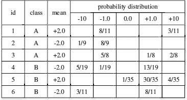
Algorithm: Let us first use an example to illustrate how decision trees can be used for classifying uncertain data. Suppose that there are six tuples with given labels A or B (Figure 16.1). Each tuple has a single uncertain attribute. After sampling its pdf for a few times, its probability distribution is approximated by five values with probabilities, as shown in the figure. Notice that the mean values of attributes tuples 1, 3 and 5 are the same, i.e., 2.0. However, their probability distributions are different.

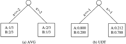
We first use these tuples as a training dataset, and consider the method AVG. Essentially, we only use these tuples’ mean values to build a decision tree based on traditional algorithms such as C4.5 [28] (Figure 16.2(a)). In this example, the split point is x = −2. Conceptually, this value determines the branch of the tree used for classifying a given tuple. Each leaf node contains the information about the probability of an object to be in each class. If we use this decision tree to classify tuple 1, we will reach the right leaf node by traversing the tree, since its mean value is 2.0. Let P(A) and P(B) be the probabilities of a test tuple for belonging to classes A and B, respectively. Since P(A) = 2/3, which is greater than P(B) = 1/3, we assign tuple 1 with label “A.” Using a similar approach, we label tuples 1, 3, and 5 as “A,” and name tuples 2, 4, 6 as “B.”. The number of tuples classified correctly, i.e., tuples 1, 3, 4 and 6, is 4, and the accuracy of AVG in this example is 2/3.

The form of the decision tree trained by UDT is in fact the same as the one constructed through AVG. In our previous example, the decision tree generated by UDT is shown in Figure 16.2(b). We can see that the only difference from (a) is that the split point is x = -1, which is different from that of AVG. Let us now explain (1) how to use UDT to train this decision tree; and (2) how to use it to classify previously unseen tuples.

1. Training Phase. This follows the framework of C4.5 [28]. It builds decision trees from the root to the leaf nodes in a top-down, recursive, and divide-and-conquer manner. Specifically, the training set is recursively split into smaller subsets according to some splitting criterion,in order to create subtrees. The splitting criterion is designed to determine the best way to partition the tuples into individual classes. The criterion not only tells us which attribute to be tested, but also how to use the selected attribute (by using the split point). We will explain this procedure in detail soon. Once the split point of a given node has been chosen, we partition the dataset into subsets according to its value. In Figure 16.2(a), for instance, we classify tuples with x > −2 to the right branch, and put tuples with x < −2 to the left branch. Then we create new sub-nodes with the subsets recursively. The commonly used splitting criteria are based on indexes such as information gain (entropy), gain ratio, and Gini index. Ideally, a good splitting criterion should make the resulting partitions at each branch as “pure”as possible (i.e., the number of distinct objects that belong to the branch is as few as possible).

   Let us now explain how to choose an attribute to split, and how to split it. First, assume that an attribute is chosen to split, and the goal is to find out how to choose the best split point for an uncertain attribute. To do this, UDT samples points from the pdf of the attribute, and considers them as candidate split points. It then selects the split point with the lowest entropy. The computation of entropy H(q,Aj) for a given split point q over an attribute Aj is done as follows: first split the dataset into different subsets according to the split point. Then for each subset, we compute its probabilities of belonging to different classes. Then its entropy H(q, Aj) can be computed based on these probabilities. The optimal split point is the one that minimizes the entropy for Aj. Notice that this process can potentially generate more candidate split points than that of AVG, which is more expensive but can be more accurate [32]. In the above example, to choose the best split point, we only have to check 2 points in AVG since the attributes concerned only have two distinct values, 2 and -2. On the other hand, we have to check five distinct values in UDT.

   How to choose the attribute for which a split point is then applied? This is done by first choosing the optimal split points for all the attributes respectively, and then select the attribute whose entropy based on its optimal split point is the minimum among those of other attributes. After an attribute and a split point have been chosen for a particular node, we split the set S of objects into two subsets, L and R. If the pdf of a tuple contains the split point x, we split it into two fractional tuples [28] tL and tR, and add them to L and R, respectively. For example, for a given tuple xi, let the interval of its j- attribute Aj be [li,j, ri,j], and the split point be li,j < p < ri,j. After splitting, we obtain two fractional tuples, whose attributes have intervals li,j, p] and (p, ri,j]. The pdf of attribute Aj of a fractional tuple xf is the same as the one defined for xi, except that the pdf value is equal to zero outside the interval of the fractional tuple’s attribute (e.g., li,j, p]). After building the tree by the above steps, some branches of a decision tree may reflect anomalies in the training data due to noise or outliers. In this case, traditional pruning techniques, such as pre-pruning and post-pruning [28], can be adopted to prune these nodes.

2. Testing Phase. For a given test tuple with uncertainty, there may be more than one path for traversing the decision tree in a top-down manner (from the root node). This is because a node may only cover part of the tuple. When we visit an internal node, we may split the tuple into two parts at its split point, and distribute each part recursively down the child nodes accordingly. When the leaf nodes are reached, the probability distribution at each leaf node contributes to the final distribution for predicting its class label.1

To illustrate this process, let us consider the decision tree in Figure 16.2(b) again, where the split point is x = − 1. If we use this decision tree to classify tuple 1 by its pdf, its value is either -1 with probability 8/11, or 10 with probability 3/11. After traversing from the root of the tree, we will reach the left leaf node with probability 8/11, and the right leaf node with probability 3/11. Since the left leaf node has a probability 0.8 of belonging to class A, and right leaf node has a probability 0.212 of belonging to class A, $\mathit{P}\mathrm{(}\mathit{A}\mathrm{)}\mathrm{=}\mathrm{(}\mathrm{8}\mathrm{/}\mathrm{1}\mathrm{1}\mathrm{)}\mathrm{\times }\mathrm{0}\mathrm{.}\mathrm{8}\mathrm{+}\mathrm{(}\mathrm{3}\mathrm{/}\mathrm{1}\mathrm{1}\mathrm{)}\mathrm{\times }\mathrm{0}\mathrm{.}\mathrm{2}\mathrm{1}\mathrm{2}\mathrm{=}\mathrm{0}\mathrm{.}\mathrm{6}\mathrm{4}$. We can similarly compute $\mathit{P}\mathrm{(}\mathit{B}\mathrm{)}\mathrm{=}\mathrm{(}\mathrm{8}\mathrm{/}\mathrm{1}\mathrm{1}\mathrm{)}\mathrm{\times }\mathrm{0}\mathrm{.}\mathrm{2}\mathrm{+}\mathrm{(}\mathrm{3}\mathrm{/}\mathrm{1}\mathrm{1}\mathrm{)}\mathrm{\times }\mathrm{0}\mathrm{.}\mathrm{7}\mathrm{8}\mathrm{8}\mathrm{=}\mathrm{0}\mathrm{.}\mathrm{3}\mathrm{6}$. Since $\mathit{P}\mathrm{(}\mathit{A}\mathrm{)}\mathrm{>}\mathit{P}\mathrm{(}\mathit{B}\mathrm{)}$ , tuple 1 is labelled as “A”.

Efficient split point computation. By considering pdf during the decision tree process, UDT promises to build a more accurate decision tree than AVG. Its main problem is that it has to consider a lot more split points than AVG, which reduces its efficiency. In order to accelerate the speed of finding the best split point, [32] proposes several strategies to prune candidate split points. To explain, suppose that for a given set S of tuples, the interval of the j-th attribute of the i-th tuple in S is represented as $\mathrm{[}{\mathit{l}}_{\mathit{i}\mathrm{,}\mathit{j}}\mathrm{,}{\mathit{r}}_{\mathit{i}\mathrm{,}\mathit{j}}\mathrm{]}$, associated with pdf ${\mathit{f}}_{\mathit{i}}^{\mathit{j}}\mathrm{(}\mathit{x}\mathrm{)}$ . The set of end-points of objects in s on attribute Aj can be defined as ${\mathit{Q}}_{\mathit{j}}\mathrm{=}\mathrm{\left\{}\mathit{q}\mathrm{\right|}\mathrm{(}\mathit{q}\mathrm{=}{\mathit{l}}_{\mathit{i}\mathrm{,}\mathit{j}}\mathrm{)}\mathrm{\vee }\mathrm{(}\mathit{q}\mathrm{=}{\mathit{r}}_{\mathit{i}\mathrm{,}\mathit{j}}\mathrm{)}\mathrm{\}}$. Points that lie in $\mathrm{(}{\mathit{l}}_{\mathit{i}\mathrm{,}\mathit{j}}\mathrm{,}\mathrm{}{\mathit{r}}_{\mathit{i}\mathrm{,}\mathit{j}}\mathrm{)}$ are called interior points. We assume that there are v end-points, ${\mathit{q}}_{\mathrm{1}}\mathrm{,}{\mathit{q}}_{\mathrm{2}}\mathrm{\text{...}}{\mathit{q}}_{\mathit{v}}$, sorted in ascending order. Our objective is to find an optimal split point in $\mathrm{[}{\mathit{q}}_{\mathrm{1}}\mathrm{,}{\mathit{q}}_{\mathit{v}}\mathrm{]}\mathrm{.}$

The end-points define v−1 disjoint intervals: $\mathrm{(}{\mathit{q}}_{\mathit{k}}\mathrm{,}{\mathit{q}}_{\mathit{k}\mathrm{+}\mathrm{1}}\mathrm{]}$, where $\mathrm{1}\mathrm{\le }\mathit{k}\mathrm{\le }\mathit{v}\mathrm{-}\mathrm{1}\mathrm{.}$ [32] defines three types of interval: empty, interval and heterogeneous. An interval $\mathrm{(}{\mathit{q}}_{\mathit{k}}\mathrm{,}{\mathit{q}}_{\mathit{k}\mathrm{+}\mathrm{1}}\mathrm{]}$ is called empty if the probability on this interval ${{\displaystyle \int }}_{{\mathit{q}}_{\mathit{k}}}^{{\mathit{q}}_{\mathit{k}\mathrm{+}\mathrm{1}}}{\mathit{f}}_{\mathit{i}}^{\mathit{j}}\mathrm{(}\mathit{x}\mathrm{)}\mathit{d}\mathit{x}\mathrm{=}\mathrm{0}$ for all ${\mathit{x}}_{\mathit{i}}\mathrm{\in }\mathit{S}$. An interval $\mathrm{(}{\mathit{q}}_{\mathit{k}}\mathrm{,}{\mathit{q}}_{\mathit{k}\mathrm{+}\mathrm{1}}\mathrm{]}$ is homogeneous if there exists a class label $\mathit{c}\mathrm{\in }\mathit{C}$ such that the probability on this interval ${\int }_{q_k}^{q_{k+1}}{f}_i^j\left(x\right)dx\ne 0\Rightarrow C_i=c$ for all ${\mathit{x}}_{\mathit{i}}\mathrm{\in }\mathit{S}$. An interval $\mathrm{(}{\mathit{q}}_{\mathit{k}}\mathrm{,}{\mathit{q}}_{\mathit{k}\mathrm{+}\mathrm{1}}\mathrm{]}$ is heterogeneous if it is neither empty nor homogeneous. We next discuss three techniques for pruning candidate split points.

1. Pruning empty and homogeneous intervals. [32] shows that empty and homogeneous in- tervals do not need to be considered. In other words, the interior points of empty and homogeneous intervals can be ignored.
2. Pruning by bounding. This strategy removes heterogeneous intervals through a bounding technique. The main idea is to compute the entropy $\mathit{H}\mathrm{(}\mathit{q}\mathrm{,}{\mathit{A}}_{\mathit{j}}\mathrm{)}$ for all end-points $\mathit{q}\mathrm{\in }{\mathit{Q}}_{\mathit{j}}$. Let ${\mathit{H}}_{\mathit{j}}^{\mathrm{*}}$ be the minimum value. For each heterogeneous interval (a,b], a lower bound, Lj, of H(z,Aj) over all candidate split points $\mathit{z}\mathrm{\in }\mathrm{(}{\mathit{q}}_{\mathit{k}}\mathrm{,}{\mathit{q}}_{\mathit{k}\mathrm{+}\mathrm{1}}\mathrm{]}$ is computed. An efficient method of finding Lj without considering all the candidate split points inside the interval is detailed in [33]. If $L_j\ge H_j^{*}$, none of the candidate split points within the interval $\mathrm{(}{\mathit{q}}_{\mathit{k}}\mathrm{,}{\mathit{q}}_{\mathit{k}\mathrm{+}\mathrm{1}}\mathrm{]}$ can give an entropy smaller than ${\mathit{H}}_{\mathit{j}}^{\mathrm{*}}$; therefore, the whole interval can be pruned. Since the number of end-points is much smaller than the total number of candidate split points, many heterogeneous intervals are pruned in this manner, which also reduces the number of entropy computations.
3. End-point sampling. Since many of the entropy calculations are due to the determination of entropy at the end-points, we can sample a portion (say, 10%) of the end-points, and use their entropy values to derive a pruning threshold. This method also reduces the number of entropy calculations, and improves the computational performance.

Discussions: From Figures 16.1 and 16.2, we can see that the accuracy of UDT is higher than that of AVG, even though its time complexity is higher than that of AVG. By considering the sampled points of the pdfs, UDT can find better split points and derive a better decision tree. In fact, the accuracy of UDT depends on the number of sampled points; the more points are sampled, the accuracy of UDT is closer to that of PW. In the testing phase, we have to track one or several paths in order to determine its final label, because an uncertain attribute may be covered by several tree nodes. Further experiments on ten real datasets taken from the UCI Machine Learning Repository [6] show that UDT builds more accurate decision trees than AVG does. These results also show that the pruning techniques discussed above are very effective. In particular, the strategy that combines the above three techniques reduces the number of entropy calculations to 0.56%-28% (i.e., a pruning effec- tiveness ranging from 72% to 99.44%). Finally, notice that UDT has also been extended to handle pmf in [33]. This is not difficult, since UDT samples a pdf into a set of points. Hence UDT can easily be used to support pmf

We conclude this section by briefly describing two other decision tree algorithms designed for uncertain data. In [23], the authors enhance the traditional decision tree algorithms and extend measures, including entropy and information gain, by considering the uncertain data’s intervals and pdf values. It can handle both numerical and categorical attributes. It also defines a “probabilistic entropy metric” and uses it to choose the best splitting point. In [24], a decision-tree based classification system for uncertain data is presented. This tool defines new measures for constructing, pruning, and optimizing a decision tree. These new measures are computed by considering pdfs. Based on the new measures, the optimal splitting attributes and splitting values can be identified.

16.3.2 Rule-Based Classification

Overview: Rule-based classification is widely used because the extracted rules are easy to understand. It has been studied for decades [12], [14]. A rule-based classification method often creates a set of IF-THEN rules, which show the relationship between the attributes of a dataset and the class labels during the training stage, and then uses it for classification. An IF-THEN rule is an expression of the form

IF condition THEN conclusion.

The former “IF”-part of a rule is the rule antecedent, which is a conjunction of the attribute test conditions. The latter “THEN"-part is the rule consequent, namely the predicted label under the condition shown in the “IF”-part. If a tuple can satisfy the condition of a rule, we say that the tuple is covered by the rule. For example, a database that can predict whether a person will buy computers or not may contain attributes age and pro f ession, and two labels yes and no of the class buy_computer. A typical rule may be (age = youth) ^ (pro f ession = student) ⇒ buy_computer = yes, which means that for a given tuple about a customer, if its values of attributes age and pro f ession are youth and student, respectively, we can predict that this customer will buy computers because the corresponding tuple about this customer is covered by the rule.

Most of the existing rule-based methods use the sequential covering algorithm to extract rules. The basic framework of this algorithm is as follows. For a given dataset consisting of a set of tuples, we extract the set of rules from one class at a time, which is called the procedure of Learn_One_Rule. Once the rules extracted from a class are learned, the tuples covered by the rules are removed from the dataset. This process repeats on the remaining tuples and stops when there is not any tuple. The classical rule-based method RIPPER [12] has been extended for uncertain data classification in [25], [26] which is called uRule. We will introduce uRule in this section.

Input: A set of labeled objects whose uncertain attributes are associated with pdf models or pmf models.

Algorithm: The algorithm uRule extracts the rules from one class at a time by following the basic framework of the sequential covering approach from the training data. That means we should first extract rules from class C1 by Learn_One_Rule, and then repeat this procedure for all the other classes C2,C3…CL in order to obtain all the rules. We denote the set of training instances with class label Ck as Dk,1 < k < L. Notice that these generated rules may perform well on the training dataset, but may not be effective on other data due to overfitting. A commonly used solution for this problem is to use a validation set to prune the generated rules and thus improve the rules’ quality. Hence, the Learn_One_Rule procedure includes two phases: growing and pruning. It splits the input dataset into two subsets: grow_Dataset and prune_Dataset before generating rules. The grow_Dataset is used to generate rules, and the prune_Dataset is used to prune some conjuncts, and boolean expressions between attributes and values, from these rules.

For a given sub-training dataset $D_k\left(1\le k\le L\right)$, the Learn_One_Rule procedure performs the following steps: (1) Split Dk into grow_Dataset and prune_Dataset; (2) Generate a rule from grow_Dataset; (3) Prune this rule based on prune_Dataset; and (4) Remove objects covered by the pruned rule from Dk and add the pruned rule to the final rule set. The above four steps will be repeated until there is not any tuple in the Dk. The output is a set of rules extracted from Dk.

1. Rules Growing Phase. uRule starts with an initial rule: $\mathrm{\left\{}\mathrm{\right\}}\mathrm{\Rightarrow }{\mathit{C}}_{\mathit{k}}$, where the left side is an empty set and the right side contains the target class label Ck. New conjuncts will subsequently be added to the left set. uRule uses the probabilistic information gain as a measure to identify the best conjunct to be added into the rule antecedent (We will next discuss this measure in more detail). It selects the conjunct that has the highest probabilistic information gain, and adds it as an antecedent of the rule to the left set. Then tuples covered by this rule will be removed from the training dataset Dk. This process will be repeated until the training data is empty or the conjuncts of the rules contain all the attributes. Before introducing probability information gain, uRule defines the probability cardinalities for attributes with pdf model as well as pmf model.

(a) pdf model. For a given attribute associated with pdf model, its values are represented by a pdf with an interval so a conjunct related to an attribute associated with pdf model covers an interval. For example, a conjunct of a rule for the attribute income may be 1000 ≤ income < 2000 The maximum and the minimum values of the interval are called end-points. Suppose that there are N end-points for an attribute after eliminating duplication; then this attribute can be divided into N+1 partitions. Since the leftmost and rightmost partitions do not contain data instances at all, we only need to consider the remaining N−1 partitions. We let each candidate conjunct involve a partition when choosing the best conjunct for an attribute, so there are N−1 candidate conjuncts for this attribute.

For a given rule R extracted from Dk, we call the instances in Dk that are covered and classified correctly by R positive instances, and call the instances in Dk that are covered, but are not classified correctly by R, negative instances. We denote the set of positive instances of R w.r.t. Dk as Pk, and denote the set of negative instances of R w.r.t. Dk as Nk.

For a given attribute Aj with pdf model, the probability cardinality of all the positive instances over one of its intervals $\mathrm{[}\mathit{a}\mathrm{,}\mathit{b}\mathrm{)}$ can be computed as ${\displaystyle \sum _{l=1}^{\left|P_k\right|}P\left(x_l^j\in [a,b)\wedge c_l=C_k\right)}$, and the probability cardinality of all the negative instances over the interval $\mathrm{[}\mathit{a}\mathrm{,}\mathit{b}\mathrm{)}$ can be computed as ${\displaystyle \sum _{l=1}^{\left|N_k\right|}P\left(x_l^j\in [a,b)\wedge c_l=C_k\right)}$. We denote the former as $\mathit{P}{\mathit{C}}^{\mathrm{+}}\mathrm{(}\mathrm{[}\mathit{a}\mathrm{,}\mathit{b}\mathrm{)}\mathrm{)}$ and the latter as $\mathit{P}{\mathit{C}}^{\mathrm{-}}\mathrm{(}\mathrm{[}\mathit{a}\mathrm{,}\mathit{b}\mathrm{)}\mathrm{)}$.

(b) pmf model. For a given attribute associated with pmf model, its values are represented by a set of discrete values with probabilities. Each value is called as a candidate split point. A conjunct related to an attribute associated with pmf model only covers one of its values. For example, a conjunct of a rule for the attribute pro f ession may be pro f ession=student. To choose the best split point for an attribute, we have to consider all its candidate split points. Similar to the case of pdf model, we have the following definitions.

For a given attribute Aj with pmf model, the probability cardinality of all the positive instances over one of its values v can be computed as ${\displaystyle \sum _{l=1}^{\left|P_k\right|}P\left(x_l^j=v\wedge c_l=C_k\right)}$, and the probability cardinality of all the negative instances over value v can be computed as ${\displaystyle \sum _{l=1}^{\left|N_k\right|}P\left(x_l^j=v\wedge c_l=C_k\right)}$. We denote the former as $\mathit{P}{\mathit{C}}^{\mathrm{+}}\mathrm{(}\mathit{v}\mathrm{)}$ and the latter as $\mathit{P}{\mathit{C}}^{\mathrm{-}}\mathrm{(}\mathit{v}\mathrm{)}$.

Now let us discuss how to choose the best conjunct for a rule R in the case of a pdf model (the method for pmf model is similar). We consider all the candidate conjuncts related to each attribute. For each candidate conjunct, we do the following two steps:

• (1) We compute the probability cardinalities of the positive and negative instances of R over the covered interval of this conjunct, using the method shown in (a). Let us denote the probability cardinalities on R’s positive and negative instances as $\mathit{P}{\mathit{C}}^{\mathrm{+}}\mathrm{(}\mathit{R}\mathrm{)}$ and $\mathit{P}{\mathit{C}}^{\mathrm{-}}\mathrm{(}\mathit{R}\mathrm{)}$.
• (2) We form a new rule R′ by adding this conjunct to R. Then we compute the probability cardinalities of R’s positive and negative instances over the covered interval of this conjunct respectively. Let us denote the former as $\mathit{P}{\mathit{C}}^{\mathrm{+}}\mathrm{(}\mathit{R}\mathrm{\prime }\mathrm{)}$ and the latter as $\mathit{P}{\mathit{C}}^{\mathrm{-}}\mathrm{(}\mathit{R}\mathrm{\prime }\mathrm{)}$. Then we use Definition 1 to compute the probabilistic information gain between R and R′.

Among all the candidate conjuncts of all the attributes, we choose the conjunct with the highest probabilistic information gain, which is defined as Definition 1, as the best conjunct of R,and then add it to R.

De f inition 1. Let R’ be a rule by adding a conjunct to R. The probabilistic information gain between R and R′ over the interval or split point related to this conjunct is

$$\begin{array}{ccc}\mathrm{Pr}obIn\left(R,R^{\prime }\right)=P{C}^{+}\left(R^{\prime }\right)\cdot \left[{\mathit{\text{log}}}_2\frac{P{C}^{+}\left(R^{\prime }\right)}{P{C}^{+}\left(R^{\prime }\right)+P{C}^{-}\left(R^{\prime }\right)}-{\mathit{\text{log}}}_2\frac{P{C}^{+}\left(R\right)}{P{C}^{+}\left(R\right)+P{C}^{-}\left(R\right)}\right].& & \left(16.1\right)\end{array}$$

From De f inition 1, we can see that the probabilistic information gain is proportional to $P{C}^{+}\left(R^{\prime }\right)$ and $\frac{P{C}^{+}\left(R^{\prime }\right)}{P{C}^{+}\left(R^{\prime }\right)+P{C}^{-}\left(R^{\prime }\right)}$ so it Prefers that have high accuracies.

2. Rule Pruning Phase. After extracting a rule from grow_Dataset, we have to conduct pruning on it because it may perform well on grow_Dataset, but it may not perform well in the test phase. So we should prune some conjuncts of it based on its performance on the validation set prune_Dataset. For a given rule R in the pruning phase, uRule starts with its most recently added conjuncts when considering pruning. For each conjunct of R’s condition, we consider a new rule R′ by removing it from R. Then we use R′ and R to classify the prune_Dataset, and get the set of positive instances and the set of negative instances of them. If the proportion of positive instances of R′ is larger than that of R, it means that the accuracy can be improved by removing this conjunct, so we remove this conjunct from R and repeat the same pruning steps on other conjuncts of R, otherwise we keep it and stop the pruning.

3. Classification Phase. Once the rules are learnt from the training dataset, we can use them to classify unlabeled instances. In traditional rule-based classifications such as RIPPER [12], they often use the first rule that covers the instance to predict the label. However, an uncertain data object may be covered by several rules, and so we have to consider the weight of an object covered by different rules (conceptually, the weight here is the probability that an instance is covered by a rule; for details, please read [25]), and then assign the class label of the rule with the highest weight to the instance.

Discussions: The algorithm uRule follows the basic framework of the traditional rule-based classification algorithm RIPPER [12]. It extracts rules from one class at a time by the Learn_One_Rule procedure. In the Learn_One_Rule procedure, it splits the training dataset into grow_Dataset, and prune_Dataset, generates rules from grow_Dataset and prunes rules based on prune_Dataset. To choose the best conjunct when generating rules, uRule proposes the concept of probability cardinality, and uses a measure called probabilistic information gain, which is based on probability cardinality, to choose the best conjunct for a rule. In the test phase, since a test object may be covered by one or several rules, uRule has considered the weight of coverage for final classification. Their experimental results show that this method can achieve relative stable accuracy even though the extent of uncertainty reaches 20%. So it is very robust in cases which contain large ranges of uncertainty.

16.3.3 Associative Classification

Overview: Associative classification is based on frequent pattern mining. The basic idea is to search for strong associations between frequent patterns (conjunctions of a set of attribute-value pairs) and class labels [17]. A strong association is generally expressed as a rule in the form $p_1\wedge p_2\wedge \cdots \wedge p_s\Rightarrow c_k$ called association rule, where the rule consequent ck ε C is a class label. Typical associative classification algorithms are, for example, CBA [21], CMAR [22], and HARMONY [35]. Strong associations are usually detected by identifying patterns covering a set of attribute-value pairs and a class label associated with this set of attribute-value pairs that frequently appear in a given database.

The basic algorithm for the detection of such rules works as follows: Given a collection of attribute-value pairs, in the first step the algorithm identifies the complete set of frequent patterns from the training dataset, given the user-specified minimum support threshold and/or discriminative measurements like the minimum confidence threshold. Then, in the second step a set of rules are selected based on several covering paradigms and discrimination heuristics. Finally, the rules for classification extracted in the first step can be used to classify novel database entries or for training other classifiers. In many studies, associative classification has been found to be more accurate than some traditional classification algorithms, such as decision tree, which only considers one attribute at a time, because it explores highly confident associations among multiple attributes.

In the case of uncertain data, specialized associative classification solutions are required. The work called HARMONY proposed in [35] has been extended for uncertain data classification in [16], which is called uHARMONY. It efficiently identifies discriminative patterns directly from uncertain data and uses the resulting classification features/rules to help train either SVM or rule- based classifiers for the classification procedure.

Input: A set of labeled objects whose uncertain attributes are associated with pmf models.

Algorithm: uHARMONY follows the basic framework of algorithm HARMONY [35]. The first step is to search for frequent patterns. Traditionally an itemset y is said to be supported by a tuple xi if $\mathit{y}\mathrm{\subseteq }{\mathit{x}}_{\mathit{i}}$. For a given certain database D consisting of n tuples $x_1,x_2,\cdots ,x_n$. The label of xi is denoted by ci. $\mathrm{\left|}\mathrm{\right\{}{\mathit{x}}_{\mathit{i}}\mathrm{|}{\mathit{x}}_{\mathit{i}}\mathrm{\subseteq }\mathit{D}\mathrm{\wedge }\mathit{y}\mathrm{\subseteq }{\mathit{x}}_{\mathit{i}}\mathrm{\}}\mathrm{|}$ is called the support of itemset y with respect to D, denoted by supy. The support value of itemset y under class c is defined as $\mathrm{\left|}\mathrm{\right\{}{\mathit{x}}_{\mathit{i}}\mathrm{|}{\mathit{c}}_{\mathit{i}}\mathrm{=}\mathit{c}\mathrm{\wedge }{\mathit{x}}_{\mathit{i}}\mathrm{\subseteq }\mathit{D}\mathrm{\wedge }\mathit{y}\mathrm{\subseteq }{\mathit{x}}_{\mathit{i}}\mathrm{\}}\mathrm{|}\mathrm{,}$ denoted by ${\mathit{\text{sup}}}_x^c\cdot y$ is said to be frequent if ${\sup }_{\mathit{x}}\mathrm{\ge }{\sup }_{\min }$, where supmin is a user specified minimum support threshold. The confidence of y under class c can be defined as $\mathit{c}\mathit{o}\mathit{n}{\mathit{f}}_{\mathit{y}}^{\mathit{c}}\mathrm{=}{\sup }_{{\mathit{y}}^{\mathbf{C}}}\mathrm{/}{\sup }_{\mathit{y}}\mathrm{.}$

However, for a given uncertain database, there exists a probability of $\mathit{y}\mathrm{\subseteq }{\mathit{x}}_{\mathit{i}}$ when y contains at least one item of uncertain attribute, and the support of y is no longer a single value but a probability distribution function instead. uHARMONY defines pattern frequentness by means of the expected support and uses the expected confidence to represent the discrimination of found patterns.

1. Expected Confidence. For a given itemset y on the training dataset, its expected support $\mathit{E}\mathrm{(}{\sup }_{\mathit{y}}\mathrm{)}$ is defined as $\mathit{E}\mathrm{(}{\sup }_{\mathit{y}}\mathrm{)}\mathrm{=}\underset{\mathit{i}\mathrm{=}\mathrm{1}}{\overset{\mathit{n}}{{\displaystyle \Sigma }}}\mathit{P}\mathrm{(}\mathit{y}\mathrm{\subseteq }{\mathit{x}}_{\mathit{i}}\mathrm{)}$. Its expected support on class c is defined as $\mathit{E}\mathrm{(}{\sup }_{{\mathit{y}}^{\mathbf{C}}}\mathrm{)}\mathrm{=}\underset{\mathit{i}\mathrm{=}\mathrm{1}}{\overset{\mathit{n}}{{\displaystyle \Sigma }}}\mathrm{(}\mathit{P}\mathrm{(}\mathit{y}\mathrm{\subseteq }{\mathit{x}}_{\mathit{i}}\mathrm{)}\mathrm{\wedge }{\mathit{c}}_{\mathit{i}}\mathrm{=}\mathit{c}\mathrm{)}$. Its expected confidence can be defined as Definition 1.

De f inition 1. Given a set of objects and the set of possible worlds W with respect to it, the expected confidence of an itemset y on class c is

$$\begin{array}{ccc}E\left({\mathit{\text{conf}}}_y{}^c\right)={\displaystyle \sum _{w_i\in W}{\mathit{\text{conf}}}_{y,w_i}{}^c\times P\left(w_i\right)=}{\displaystyle \sum _{w_i\in W}\frac{{\mathit{\text{sup}}}_{y,w_i}{}^c}{{\mathit{\text{sup}}}_{y,w_i}}\times P\left(w_i\right)}& & \left(16.2\right)\end{array}$$

where P(wi) stands for the probability of world $w_i;con{f}_{y,w_i}{}^c$ is the confidence of y on class c in world wi, while ${\sup }_{\mathit{y}\mathrm{,}{\mathit{w}}_{\mathit{i}}}\mathrm{(}{\sup }_{\mathit{y}\mathrm{,}{\mathit{w}}_{\mathit{i}}^{\mathbf{C}}}\mathrm{)}$ is the support of x (on class c) in world wi.

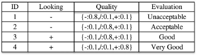
For a given possible world wi $con{f}_{y,w_i}{}^c$, ${\mathit{sup}}_{\mathit{y}\mathrm{,}{\mathit{w}}_{\mathit{i}}^{\mathbf{C}}}$, and ${\mathit{sup}}_{\mathit{y}\mathrm{,}{\mathit{w}}_{\mathit{i}}}$ can be computed using the traditional method as introduced in the previous paragraph. Although we have $\mathit{c}\mathit{o}\mathit{n}{\mathit{f}}_{\mathit{y}}^{\mathit{c}}\mathrm{=}{\mathit{sup}}_{{\mathit{y}}^{\mathbf{C}}}\mathrm{/}{\mathit{sup}}_{\mathit{y}}$ on a certain database, the expected confidence $\mathit{E}\mathrm{(}\mathit{c}\mathit{o}\mathit{n}{\mathit{f}}_{\mathit{y}}^{\mathit{c}}\mathrm{)}\mathrm{=}\mathit{E}\mathrm{(}{\mathit{sup}}_{{\mathit{y}}^{\mathbf{C}}}\mathrm{/}{\mathit{sup}}_{\mathit{y}}\mathrm{)}$ of itemset y on class c is not equal to $\mathit{E}\mathrm{(}{\mathit{sup}}_{{\mathit{y}}^{\mathbf{C}}}\mathrm{)}\mathrm{/}\mathit{E}\mathrm{(}{\mathit{sup}}_{\mathit{y}}\mathrm{)}$ on an uncertain database. For example, Figure 16.3 shows an uncertain database about computer purchase evaluation with a certain attribute on looking and an uncertain attribute on quality. The column named Evaluation represents the class labels. For the example of tuple 1, the probabilities of Bad, Medium, and Good qualities are 0.8, 0.1 and 0.1 respectively.

Let us consider the class c=Unacceptable, and the itemset y={Looking = −, Quality = −}, which means the values of the attributes Looking and Quality are Bad in the itemset y. In order to compute the expected confidence $\mathit{E}\mathrm{(}\mathit{c}\mathit{o}\mathit{n}{\mathit{f}}_{\mathit{y}}^{\mathit{c}}\mathrm{)}$, we have to consider two cases that contain y (notice that we will not consider cases that do not contain y since their expected support and expected confidence is 0.). Let casel denote the first case in which the first two tuples contain y and the other two tuples do not contain y, so the probability of case1 is $\mathit{P}\mathrm{(}\mathit{c}\mathit{a}\mathit{s}\mathit{e}\mathrm{1}\mathrm{)}\mathrm{=}\mathrm{0}\mathrm{.}\mathrm{8}\mathrm{\times }\mathrm{0}\mathrm{.}\mathrm{1}$. Since only one tuple in w1, i.e., tuple 1, has the label c = Unacceptable, ${\mathit{sup}}_{\mathit{y}\mathrm{,}\mathit{c}\mathit{a}\mathit{s}\mathit{e}{\mathrm{1}}^{\mathbf{C}}}\mathrm{=}\mathrm{1}$ and ${\mathit{sup}}_{\mathit{y}\mathrm{,}\mathit{c}\mathit{a}\mathit{s}\mathit{e}\mathrm{1}}\mathrm{=}\mathrm{2}\mathrm{.}$ Let case2 denote the second case in which only the first one tuple contains y and the other three tuples do not contain y, so the probability of case2 is $\mathit{P}\mathrm{(}\mathit{c}\mathit{a}\mathit{s}\mathit{e}\mathrm{2}\mathrm{)}\mathrm{=}\mathrm{0}\mathrm{.}\mathrm{8}\mathrm{\times }\mathrm{0}\mathrm{.}\mathrm{9}{\sup }_{\mathit{y}\mathrm{,}\mathit{c}\mathit{a}\mathit{s}\mathit{e}{\mathrm{2}}^{\mathit{c}}}\mathrm{=}\mathrm{1}$ and ${\sup }_{\mathit{y}\mathrm{,}\mathit{c}\mathit{a}\mathit{s}\mathit{e}\mathrm{2}}\mathrm{=}\mathrm{1}$. So we can calculate $\mathit{E}\mathrm{(}\mathit{c}\mathit{o}\mathit{n}{\mathit{f}}_{\mathit{y}}^{\mathit{c}}\mathrm{)}\mathrm{=}\mathrm{1}\mathrm{.}\mathrm{0}\mathrm{\times }\mathrm{(}\mathrm{0}\mathrm{.}\mathrm{8}\mathrm{\times }\mathrm{0}\mathrm{.}\mathrm{9}\mathrm{)}\mathrm{+}\mathrm{0}\mathrm{.}\mathrm{5}\mathrm{\times }\mathrm{(}\mathrm{0}\mathrm{.}\mathrm{8}\mathrm{\times }\mathrm{0}\mathrm{.}\mathrm{1}\mathrm{)}\mathrm{=}\mathrm{0}\mathrm{.}\mathrm{7}\mathrm{6}$, while $\mathit{E}\mathrm{(}{\mathit{sup}}_{{\mathit{y}}^{\mathbf{C}}}\mathrm{)}\mathrm{/}\mathit{E}\mathrm{(}{\mathit{sup}}_{\mathit{y}}\mathrm{)}\mathrm{=}\mathrm{0}\mathrm{.}\mathrm{8}\mathrm{/}\mathrm{(}\mathrm{0}\mathrm{.}\mathrm{8}\mathrm{+}\mathrm{0}\mathrm{.}\mathrm{1}\mathrm{)}\mathrm{=}\mathrm{0}\mathrm{.}\mathrm{8}\mathrm{9}$. Therefore, the calculation of expected confidence is non-trivial and requires careful computation.

Unlike probabilistic cardinalities like probabilistic information gain discussed in Section 16.3.2 which may be not precise and lack theoretical explanations and statistical meanings, the expected confidence is statistically meaningful while providing a relatively accurate measure of discrimination. However, according to the De f inition 1, if we want to calculate the expected confidence of a given itemset y, the number of possible worlds $\mathrm{\left|}\mathit{W}\mathrm{\right|}$ is extremely large and it is actually exponential. The work [16] proposes some theorems to compute the expected confidence efficiently.

Lemma 1. Since $0\le {\mathit{\text{sup}}}_y{}^c\le {\mathit{\text{sup}}}_y\le n$, we have: $E\left(con{f}_y^c\right)={\displaystyle \sum _{w_i\in W}con{f}_{y,w_i}{}^c\times P\left(w_i\right)={\displaystyle \sum _{i=0}^n{\displaystyle \sum _{j=0}^i\frac{j}{i}\times P\left({\mathit{\text{sup}}}_y=i\wedge {\mathit{\text{sup}}}_y^c=j\right)={\displaystyle \sum _{i=0}^n\frac{E_i\left({\mathit{\text{sup}}}_y^c\right)}{i}={\displaystyle \sum _{i=0}^n{E}_i\left(con{f}_y{}^c\right)}}}}}$, where $E_i\left({\mathit{\text{sup}}}_y^c\right)$ and ${\mathit{E}}_{\mathit{i}}\mathrm{(}\mathit{c}\mathit{o}\mathit{n}{\mathit{f}}_{\mathit{y}}^{\mathit{c}}\mathrm{)}$ denote the part of expected support and confidence of itemset y on class c when ${\mathit{sup}}_{\mathit{y}}\mathrm{=}\mathit{i}\mathrm{.}$

Given $\mathrm{0}\mathrm{\le }\mathit{j}\mathrm{\le }\mathit{n}$, let $E_j\left({\mathit{\text{sup}}}_y{}^c\right)={\sum }_{i=0}^n{E}_{i,j}\left({\mathit{\text{sup}}}_y{}^c\right)$ be the expected support of y on class c on the first j objects of Train_D, and ${\mathit{E}}_{\mathit{i}\mathrm{,}\mathit{j}}\mathrm{(}{\mathit{sup}}_{{\mathit{y}}^{\mathbf{C}}}\mathrm{)}$ be the part of expected support of y on class c with support of i on the first j objects of Train_D.

Theorem 1. Let pi denote $\mathit{P}\mathrm{(}\mathit{y}\mathrm{\subseteq }{\mathit{x}}_{\mathit{i}}\mathrm{)}$ for each object xi ∈ Train_D, and ${\mathit{P}}_{\mathit{i}\mathrm{,}\mathit{j}}$ be the probability of y having support of i on the first j objects of Train_D. We have $E_{i,j}\left({\mathit{\text{sup}}}_y{}^c\right)=p_j\times E_{i-1,j-1}\left({\mathit{\text{sup}}}_y{}^c\right)+\left(1-p_j\right)\times E_{i,j-1}\left({\mathit{\text{sup}}}_y{}^c\right)$ when ${\mathit{c}}_{\mathit{j}}\mathrm{\ne }\mathit{c}$, and $E_{i,j}\left({\mathit{\text{sup}}}_y{}^c\right)=p_j\times E_{i-1,j-1}\left({\mathit{\text{sup}}}_y{}^c\right)+\left(1-p_j\right)\times E_{i,j-1}\left({\mathit{\text{sup}}}_y{}^c\right)$ when ${\mathit{c}}_{\mathit{j}}\mathrm{=}\mathit{c}$, where $0\le i\le j\le n.E_{i,j}\left({\mathit{\text{sup}}}_y{}^c\right)=0$ for $\mathrm{\forall }\mathit{j}$ where $\mathit{i}\mathrm{=}\mathrm{0}$, or where $\mathit{j}\mathrm{<}\mathit{i}\mathrm{.}$ (For the details of the proof, please refer to [16].)

Notice that ${\mathit{P}}_{\mathit{i}\mathrm{,}\mathit{j}}$ can be computed in a similar way as shown in Therorem 1 (for details, please refer to [16]) . Based on the above theory, we can compute the expected confidence with $\mathit{O}\mathrm{(}{\mathit{n}}^{\mathrm{2}}\mathrm{)}$ time complexity and $\mathit{O}\mathrm{(}\mathit{n}\mathrm{)}$ space complexity. In addition, the work [16] also proposes some strategies to compute the upper bound of expected confidence, which makes the computation of expected confidence more efficient.

2. Rules Mining. The steps of mining frequent itemsets of uHARMONY are very similar with HARMONY [35]. Before running the itemset mining algorithm, it sorts the attributes to place all the certain attributes before uncertain attributes. The uncertain attributes will be handled at last when extending items by traversing the attributes. During the mining process, we start with all the candidate itemsets, each of which contains only one attribute-value pair, namely a conjunct. For each candidate itemset y, we first compute its expected confidence $\mathit{E}\mathrm{(}\mathit{c}\mathit{o}\mathit{n}{\mathit{f}}_{\mathit{y}}^{\mathit{c}}\mathrm{)}$ under different classes, and then we assign the class label c* with the maximum confidence as its class label. We denote this candidate rule as y ⇒ c* and then count the number of covered instances by this rule. If the number of covered instances by this itemset is not zero, we output a final rule y ⇒ c* and remove y from the set of candidate itemsets. Based on this mined rule, we compute a set of new candidate itemsets by adding all the possible conjuncts related to other attributes to y. For each new candidate itemset, we repeat the above process to generate all the rules.

After obtaining a set of itemsets, we can use them as rules for classification directly. For each test instance, by summing up the product of the confidence of each itemset on each class and the probability of the instance containing the itemset, we can assign the class label with the largest value to it. In addition, we can convert the mined patterns to training features of other classifiers such as SVM for classification [16].

Discussions: The algorithm uHARMONY follows the basic framework of HARMONY to mine discriminative patterns directly and effectively from uncertain data. It proposes to use expected confidence of a discovered itemset to measure the discrimination. If we compute the expected confidence according to its original definition, which considers all the simple combinations of those training objects, i.e., the possible worlds, the time complexity is exponential, which is impractical in practice. So uHARMONY proposes some theorems to compute expected confidence efficiently. The overall time complexity and space complexity of computing the expected confidence of a given itemset y are at most O(n2) and O(n), respectively. Thus, it can be practical in real applications. These mined patterns can be used as classification features/rules to classify new unlabeled objects or help to train other classifiers (i.e., SVM). Their experimental results show that uHARMONY can outperform other uncertain data classification algorithms such as decision tree classification [23] and rule-based classification [25] with 4% to 10% improvement on average in accuracy on 30 categorical datasets.

16.3.4 Density-Based Classification

Overview: The basis of density-based classification are density estimation methods that provide an effective intermediate representation of potentially erroneous data capturing the information about the noise in the underlying data, and are in general useful for uncertain data mining [1]. Data mining in consideration of density in the underlying data is usually associated with clustering [17], such as density-based clustering DBSCAN [13] or hierarchical density-based clustering OPTICS [5]. These concepts form clusters by dense regions of objects in the data space separated by region of low density (usually interpreted as noise) yielding clusters of arbitrary shapes that are robust to noise. The idea of using object density information for mutual assignment of objects can also be used for classification. In the work [1], a new method is proposed for handling error-prone and missing data with the use of density estimation.

Input: A set of labeled objects whose uncertain attributes are associated with pdf models.

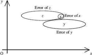
Algorithm: The presence of uncertainty or errors in the data may change the performance of classification process greatly. This can be illustrated by the two. dimensional binary classification example as shown in Figure 16.4. Suppose the two uncertain training samples y and z, whose uncertainties are illustrated by the oval regions, respectively, are used to classify the uncertain object x.A nearest-neighbor classifier would pick the class label of data point y. However, the data point z may have a much higher probability of being the nearest neighbor to x than the data point y, because x lies within the error boundary of z and outside the error boundary of y. Therefore, it is important to design a classification method that is able to incorporate potential uncertainty (errors) in the data in order to improve the accuracy of the classification process.

1. Error-Based Density Estimation. The work proposed by Aggarwal [1] introduces a general and scalable approach to uncertain data mining based on multi-variate density estimation. The kernel density estimation f(x) provides a continuous estimate of the density of the data at a given point x. An introduction of kernel density estimation is given in Section 16.3.7. Specifically, the value of the density at point x is the sum of smoothed values of kernel functions ${K^{\prime }}_h(\cdot )$ associated with each point in the data set. Each kernel function is associated with a kernel width h, which determines the level of smoothing created by the function. The kernel estimation is defined as follows:

$$\begin{array}{ccc}\overline{f}\left(x\right)=\frac{1}{n}{\displaystyle \sum _{i=1}^n{K^{\prime }}_h\left(x-x_i\right)}& & \left(16.3\right)\end{array}$$

A Gaussian kernel with width h can be defined as Equation(16.4).

$$\begin{array}{ccc}{K^{\prime }}_h\left(x-x_i\right)=\left(1/\sqrt{2\text{π}}\cdot h\right)\cdot e^{\frac{-{\left(x-x_i\right)}^2}{2h^2}}& & \left(16.4\right)\end{array}$$

The overall effect of kernel density estimation is to replace each discrete point xi by a continu- ous function ${\mathit{K}}_{\mathit{h}}\mathrm{\prime }\mathrm{(}\mathit{x}\mathrm{-}{\mathit{x}}_{\mathit{i}}\mathrm{)}$ , which peaks at $\widehat{x_i}$ and has a variance that is determined by the smoothing parameter h.

The presence of attribute-specific errors may change the density estimates. In order to take these errors into account, we need to define error-based kernels. The error-based kernel can be defined as:

$$\begin{array}{ccc}{Q^{\prime }}_h\left(x-{\stackrel{⌢}{x}}_i,\text{φ}\left(x_i\right)\right)=\left(1/\sqrt{2\text{π}}\cdot \left(h+\text{φ}\left(x_i\right)\right)\right)\cdot e^{\frac{-{\left(x-{\stackrel{⌢}{x}}_i\right)}^2}{2\left(h^2+\text{φ}{\left(x_i\right)}^2\right)}},& & \left(16.5\right)\end{array}$$

where $\mathit{\phi }\mathrm{(}{\mathit{x}}_{\mathit{i}}\mathrm{)}$ denotes the estimated error associated with data point xi.

As in the previous case, the error-based density at a given data point is defined as the sum of the error-based kernels over different data points. Consequently, the error-based density $\overline{{\mathit{f}}^{\mathit{Q}}}\mathrm{(}\mathit{x}\mathrm{,}\mathrm{}\mathit{\phi }\mathrm{(}{\mathit{x}}_{\mathit{i}}\mathrm{)}\mathrm{)}$ at point xi is defined as:

$$\begin{array}{ccc}\overline{f^Q}\left(x,\text{φ}\left(x_i\right)\right)=\left(1/N\right)\cdot {\displaystyle \sum _{i=1}^N{Q^{\prime }}_h\left(x-x_i,\text{φ}\left(x_i\right)\right)}.& & \left(16.6\right)\end{array}$$

This method can be generalized for very large data sets and data streams by condensing the data into micro-clusters; specifically, here we need to adapt the concept of micro-cluster by incorporating the error information. In the following we will define an error-based micro-cluster as follows:

De f inition 1: An error-based micro-cluster for a set of d-dimensional points $\mathit{M}\mathit{C}\mathrm{=}\mathrm{\{}{\mathit{x}}_{\mathrm{1}}\mathrm{,}{\mathit{x}}_{\mathrm{2}}\mathrm{,}\mathrm{}\cdots {\mathit{x}}_{\mathit{m}}\mathrm{\}}$ with order 1, 2, …,m is defined as a (3 . d+1) tuple $\mathrm{(}\overline{\mathit{C}\mathit{F}{\mathrm{2}}^{\mathit{x}}}\mathrm{(}\mathit{M}\mathit{C}\mathrm{)}\mathrm{,}\overline{\mathit{E}\mathit{F}{\mathrm{2}}^{\mathit{x}}}\mathrm{(}\mathit{M}\mathit{C}\mathrm{)}\mathrm{,}\overline{\mathit{C}\mathit{F}{\mathrm{1}}^{\mathit{x}}}\mathrm{(}\mathit{M}\mathit{C}\mathrm{)}\mathrm{,}\mathit{n}\mathrm{(}\mathit{M}\mathit{C}\mathrm{)}\mathrm{)}$ , wherein $\overline{\mathit{C}\mathit{F}{\mathrm{2}}^{\mathit{x}}}\mathrm{(}\mathit{M}\mathit{C}\mathrm{)}\mathrm{,}\overline{\mathit{E}\mathit{F}{\mathrm{2}}^{\mathit{x}}}\mathrm{(}\mathit{M}\mathit{C}\mathrm{)}$ , and $\overline{\mathit{C}\mathit{F}{\mathrm{1}}^{\mathit{x}}}\mathrm{(}\mathit{M}\mathit{C}\mathrm{)}$ each correspond to a vector of d entries. The definition of each of these entries is as follows.

• For each dimension, the sum of the squares of the data values is maintained in $\overline{\mathit{C}\mathit{F}{\mathrm{2}}^{\mathit{x}}}\mathrm{(}\mathit{M}\mathit{C}\mathrm{)}$ . Thus, $\overline{\mathit{C}\mathit{F}{\mathrm{2}}^{\mathit{x}}}\mathrm{(}\mathit{M}\mathit{C}\mathrm{)}$ contains d values. The p-th entry of $\overline{CF{2}^x}\left(MC\right)$ is equal to ${{\displaystyle \Sigma }}_{\mathit{i}\mathrm{=}\mathrm{1}}^{\mathit{m}}\mathrm{(}{\mathit{x}}_{\mathit{i}}^{\mathit{p}}{\mathrm{)}}^{\mathrm{2}}$.
• For each dimension, the sum of the square of the errors in data values is maintained in $\overline{\mathit{E}\mathit{F}{\mathrm{2}}^{\mathit{x}}}\mathrm{(}\mathit{M}\mathit{C}\mathrm{)}$ . Thus, $\overline{\mathit{E}\mathit{F}{\mathrm{2}}^{\mathit{x}}}\mathrm{(}\mathit{M}\mathit{C}\mathrm{)}$ contains d values. The p-th entry of $\overline{\mathit{E}\mathit{F}{\mathrm{2}}^{\mathit{x}}}\mathrm{(}\mathit{M}\mathit{C}\mathrm{)}$ is equal to ${{\displaystyle \Sigma }}_{\mathit{i}\mathrm{=}\mathrm{1}}^{\mathit{m}}\mathrm{(}{\mathit{\phi }}_{\mathit{p}}\mathrm{(}{\mathit{x}}_{\mathit{i}}\mathrm{)}{\mathrm{)}}^{\mathrm{2}}$
• For each dimension, the sum of the data values is maintained in $\overline{\mathit{C}\mathit{F}{\mathrm{1}}^{\mathit{x}}}\mathrm{(}\mathit{M}\mathit{C}\mathrm{)}$ . Thus, $\overline{\mathit{C}\mathit{F}{\mathrm{1}}^{\mathit{x}}}\mathrm{(}\mathit{M}\mathit{C}\mathrm{)}$ contains d values. The p-entry of $\overline{CF{1}^x}\left(MC\right)$ is equal to ${{\displaystyle \Sigma }}_{\mathit{i}\mathrm{=}\mathrm{1}}^{\mathit{m}}{\mathit{x}}_{\mathit{i}}^{\mathit{p}}\mathrm{.}$
• The number of points in the data is maintained in $\mathit{n}\mathrm{(}\mathit{M}\mathit{C}\mathrm{)}$ .

In order to compress large data sets into micro-clusters, we can create and maintain the clusters using a single pass of data as follows. Supposing the number of expected micro-clusters for a given dataset is q, we first randomly choose q centroids for all the micro-clusters that are empty in the initial stage. For each incoming data point, we assign it to its closest micro-cluster centroid using the nearest neighbor algorithm. Note that we never create a new micro-cluster, which is different from [2]. Similarly, these micro-clusters will never be discarded in this process, since the aim of this micro-clustering process is to compress the data points so that the resulting statistic can be held in a main memory for density estimation. Therefore, the number of micro-clusters q is defined by the amount of main memory available.

In [1] it is shown that for a given micro-cluster $MC=\left\{x_1,x_2,\cdots x_m\right\}$, its true error $\mathrm{\Delta }\left(MC\right)$ can be computed efficiently. Its value along the j-th dimension can be defined as follows:

$$\begin{array}{ccc}{\Delta }_j\left(MC\right)=\frac{\overline{CF{2}_j^x}\left(MC\right)}{m}-\frac{\overline{CF{2}_j^x}{\left(MC\right)}^2}{m}+\frac{\overline{CF{2}_j^x}\left(MC\right)}{m},& & \left(16.7\right)\end{array}$$

where $\overline{CF{2}_j^x}\left(MC\right),\overline{CF{1}_j^x}{\left(MC\right)}^2$ and $\overline{EF{2}_j^x}\left(MC\right)$ are the j-th entry of the statistics of the corresponding error-based micro-cluster MC as defined above.

The true error of a micro-cluster can be used to compute the error-based kernel function for a micro-cluster. We denote the centroid of the cluster MC by $\mathit{c}\mathrm{(}\mathit{M}\mathit{C}\mathrm{)}$. Then, we can define the kernel function for the micro-cluster MC in an analogous way to the error-based definition of a data point.

$$\begin{array}{ccc}{Q^{\prime }}_h\left(x-c\left(MC\right),\Delta \left(MC\right)\right)=\left(1/\sqrt{2\text{π}}\cdot \left(h+\Delta \left(MC\right)\right)\right)\cdot e^{\frac{-{\left(x-{\stackrel{⌢}{x}}_i\right)}^2}{2\cdot \left(h^2+\Delta {\left(MC\right)}^2\right)}}\cdot & & \left(16.8\right)\end{array}$$

If the training dataset contains the micro-clusters $M{C}_1,M{C}_2,\cdots M{C}_{m\text{'}}$ where m′ is the number of micro-clusters, then we can define the density estimate at x as follows:

$$\begin{array}{ccc}\overline{f^Q}\left(x,\Delta \left(MC\right)\right)=\left(1/N\right)\cdot {\displaystyle \sum _{i=1}^{m^{\prime }}n\left(M{C}_i\right){Q^{\prime }}_h\left(x-c{\left(M{C}_i\right)}_i,\Delta \left(x_i\right)\right).}& & \left(16.9\right)\end{array}$$

This estimate can be used for a variety of data mining purposes. In the following, it is shown how these error-based densities can be exploited for classification by introducing an error-based generalization of a multi-variate classifier.

2. Density-Based Classification. The density-based classification designs a density-based adaption of rule-based classifiers. For the classification of a test instance, we need to find relevant classification rules for it. The challenge is to use the density-based approach in order to find the particular subsets of dimensions that are most discriminatory for the test instance. So we need to find those subsets of dimensions, namely subspaces, in which the instance-specific local density of dimensions for a particular class is significantly higher than its density in the overall data. Let Di denote the objects that belong to class i. For a particular test instance x, a given subspace S, and a given training dataset D, let $\mathit{g}\mathrm{(}\mathit{x}\mathrm{,}\mathit{S}\mathrm{,}\mathit{D}\mathrm{)}$ denote the density of S and D. The process of computing the density over a given subspace S is equal to the computation of the density of the full-dimensional space while incorporating only the dimensions in S.

In the test phase, we compute the micro-clusters together with the corresponding statistic of each data set D1, … ,DL where L is the number of classes in the preprocessing step. Then, the compressed micro-clusters for different classes can be used to generate the accuracy density over different subspaces by using Equations (16.8) and (16.9). To construct the final set of rules, we can use an iterative approach to find the most relevant subspaces for classification. For the relevance of a particular subspace S we define the density-based local accuracy A(x,S,Ci) as follows:

$$\begin{array}{ccc}A\left(x,S,C_i\right)=\frac{\left|D_i\right|\cdot g\left(x,S,D_i\right)}{\left|\mathit{\text{Train}}\_D\right|\cdot \left(x,S,\mathit{\text{Train}}\_D\right)}.& & \left(16.10\right)\end{array}$$

The dominant class dom(x,S) for point x in dataset S can be defined as the class with the highest accuracy. That is,

$$\begin{array}{ccc}dom\left(x,S\right)=\text{arg }\underset{1\le i\le L}{\text{max}}A\left(x,S,C_i\right).& & \left(16.11\right)\end{array}$$

To determine all the highly relevant subspaces, we follow a bottom-up methodology to find those subspaces S that yield a high accuracy of the dominant class dom(x,S) for a given test instance x. Let Tj(1 ≤ j ≤ d) denote the set of all j-th dimensional subspaces. We will compute the relevance between x and each subspace in Tj (1 ≤ j ≤ d) in an iterative way, starting with T1 and then proceeding with $T_2,T_3,\cdots T_d$. The subspaces with high relevance can be used as rules for final classification, by assigning to a test instance x the label of the class that is the most frequent dominant class of all highly relevant subspaces of x. Notice that to make this process efficient, we can impose some constraints. In order to decide whether we should consider a subspace in the set of (j + 1)-th dimension spaces, at least one subset of it needs to satisfy the accuracy threshold requirements. Let Lj(Lj ⊆Tj) denote the subspaces that have sufficient discriminatory power for that instance, namely the accuracy is above threshold α. In order to find such subspaces, we can use Equations (16.10) and (16.11). We iterate over increasing values of j, and join the candidate set Lj with the set L1 in order to determine Tj+1. Then, we can construct Lj+1 by choosing subspaces from Tj+1 whose accuracy is above α. This process can be repeated until the set Tj+1 is empty. Finally, the sets of dimensions $L_{all}={\cup }_j{L}_j$ can be used to predict the class label of the test instance x.

To summarize the density-based classification procedure, the steps of classifying a test instance are as follows. (1) compute the micro-clusters for each data set D1,…DL only once in the preprocessing step; (2) compute the highly relevant subspaces for this test instance following the bottom-up methodology and obtain a set of subspaces Lall; (3) assign the label of the majority class in Lall to the test instance.

Discussions: Unlike other uncertain data classification algorithms [8, 29, 32], the density-based classification introduced in this section not only considers the distribution of data, but also the errors along different dimensions when estimating the kernel density. It proposes a method for error-based density estimation, and it can be generalized to large data sets cases. In the test phase, it designs a density-based adaption of the rule-based classifiers. To classify a test instance, it finds all the highly relevant subspaces and then assign the label of the majority class of these subspaces to the test instance. In addition, the error-based density estimation discussed in this algorithm can also be used to construct accurate solutions for other cases, and thus it can be applied for a variety of data management and mining applications when the data distribution is very uncertain or contains a lot of errors. In an experimental evaluation it is demonstrated that the error-based classification method not only performs fast, but also can achieve higher accuracy compared to methods that do not consider error at all, such as the nearest-neighbor-based classification method that will be introduced next.

16.3.5 Nearest Neighbor-Based Classification

Overview: The nearest neighbor-based classification method has been studied since the 1960s. Although it is a very simple algorithm, it has been applied to a variety of applications due to its high accuracy and easy implementation. The normal procedure of nearest neighbor classification method is as follows: Given a set of training instances, to classify an unlabeled instance q, we have to search for the nearest-neighbor NNTrain_D(q) of q in the training set, i.e., the training instance having the smallest distance to q, and assign the class label of NNTrain_D(q) to q. The nearest neighbor-based classification can be generalized easily to take into account the k nearest-neighbor easily, which is called k nearest neighbor classification (KNN, for short). In this case, the classification rule assigns to the unclassified instance q the class containing most of its k nearest neighbors. The KNN classification is more robust against noise compared to the simple NN classification variant. The work [4] proposes a novel nearest neighbor classification approach that is able to handle uncertain data called Uncertain Nearest Neighbor (UNN, for short) classification, which extends the traditional nearest neighbor classification to the case of data with uncertainty. It proposes a concept of nearest-neighbor class probability, which is proved to be a much more powerful uncertain object classification method than the straight-forward consideration of nearest-neighbor object probabilities.

Input: A set of labeled objects whose uncertain attributes are associated with pdf models.

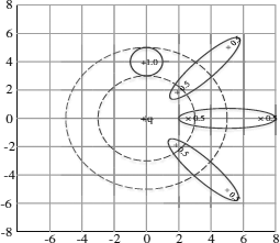
Algorithm: To extend the nearest neighbor method for uncertain data classification, it is straight-forward to follow the basic framework of the traditional nearest neighbor method and replace the distance metric method with distance between means (i.e., the expected location of the uncertain instances) or the expected distance between uncertain instances. However, there is no guarantee on the quality of the classification yielded by this naive approach. The example as shown in Figure 16.5 demonstrates that this naive approach is defective because it may misclassify. Suppose we have one certain unclassified object q, three uncertain training objects whose support is delimited by ellipsis belonging to class=“red” and another uncertain training object whose support is delimited by a circle belonging to another class=“blue”. Suppose the class=“blue” object consists of one normally distributed uncertain object whose central point is (0,4), while the class=“red” objects are bimodal uncertain objects. Following the naive approach, one can easily see that q will be assigned to the “blue” class. However, the probability that a “red”-class object is closer to q than a “blue”-class one is 1 - 0.53 = 0.875. This also indicates that the probability that the nearest neighbor of object q is a “red”-class object is 87.5%. Thus, the performance of the naive approach is quite poor as distribution information (such as the variances) of the uncertain objects is ignored.

1. Nearest Neighbor Rule for Uncertain Data. To avoid the flaws of the naive approach following the above observations, the approach in [4] proposes the concept of most probable class. It simultaneously considers the distance distributions between q and all uncertain training objects in Train_D. The probability Pr(NNTrain_D(q) = c) that the object q will be assigned to class c by means of the nearest neighbor rule can be computed as follows:

$$\begin{array}{ccc}\mathit{\text{Pr}}\left(N{N}_{Train\_D}\left(q\right)=c\right)={\displaystyle {\int }_{D^{\prime }}\mathit{\text{Pr}}\left(I_D\right)\cdot I_c\left(N{N}_{I_D}\left(q\right)\right)d{I}_D},& & \left(16.12\right)\end{array}$$

where function $I_c(\cdot )$ outputs 1 if its argument is c, and 0 otherwise, $\mathit{N}{\mathit{N}}_{{\mathit{l}}_{\mathit{D}}}\mathrm{(}\mathit{q}\mathrm{)}$ represents the label of the nearest neighbor of q in set ${\mathit{I}}_{\mathit{D}}\mathrm{,}$ $\mathit{P}\mathit{r}\mathrm{(}{\mathit{I}}_{\mathit{D}}\mathrm{)}$ represents the occurrence probability of set ${\mathit{I}}_{\mathit{D}}$, and $\mathit{D}\mathrm{\prime }$ represents all the possible combinations of training instances in Train_D. It is easy to see that the probability Pr(NNTrain_D(q) = c) is the summation of the occurrence probabilities of all the outcomes ${\mathit{I}}_{\mathit{D}}$ of the training set Train_D for which the nearest neighbor object of q in ${\mathit{I}}_{\mathit{D}}$ has class c. Note that if the domain involved in the training dataset doesn’t concide with the real number field, we can transfer the integration as summations and get Equation(16.13).

$$\begin{array}{ccc}\mathit{\text{Pr}}\left(N{N}_{Train\_D}\left(q\right)=c\right)={\displaystyle \sum _{I_D\in D^{\prime }}\mathit{\text{Pr}}\left(I_D\right)\cdot I_c\left(N{N}_{I_D}\left(q\right)\right)d{I}_D}.& & \left(16.13\right)\end{array}$$

Therefore, if we want to classify q, we should compute the probabilities Pr(NNTrain_D(q) = c) for all the classes first, and then assign it the class label ${\mathit{c}}^{\mathrm{*}}$, which is called the most probable class of q and can be computed as follows:

$$\begin{array}{ccc}{c}^{*}=\text{arg }\underset{c}{\text{max}}\mathit{\text{Pr}}\left(N{N}_{Train\_D}\left(q\right)=c\right).& & \left(16.14\right)\end{array}$$

Efficient Strategies. To classify a test object, the computational cost will be very large if we compute the probabilities using the above equations directly, so [4] introduces some efficient strategies such as the uncertain nearest neighbor (UNN) rule. Let ${\mathit{D}}_{\mathit{c}}$ denote the subset of Train_D composed of the objects having class label $\mathit{c}\mathrm{,}$ ${\mathit{D}}_{\mathit{k}}\mathrm{(}\mathit{q}\mathrm{,}\mathit{c}\mathrm{)}$ denote the distance between object q and class c (k is the number of nearest neighbors), and ${\mathit{p}}_{\mathit{i}}\mathrm{(}\mathit{R}\mathrm{)}\mathrm{=}\mathit{P}\mathit{r}\mathrm{(}\mathit{d}\mathrm{(}\mathit{q}\mathrm{,}{\mathit{x}}_{\mathit{i}}\mathrm{)}\mathrm{\le }\mathit{R}\mathrm{)}$ denote the cumulative density function representing the relative likelihood for the distance between q and training set object xi to assume value less than or equal to R. Then we have

$$\begin{array}{ccc}{p}_i\left(R\right)=\mathit{\text{Pr}}\left(d\left(q,x_i\right)\le R\right)={\displaystyle {\int }_{B_R\left(q\right)}{f}^{x_i}\left(v\right)dv}& & \left(16.15\right)\end{array}$$

where $f^{x_i}\left(v\right)$ denotes the probability for ${\mathit{x}}_{\mathit{i}}$ to assume value $\mathit{v}\mathrm{,}$ ${\mathit{B}}_{\mathit{R}}\mathrm{(}\mathit{q}\mathrm{)}$ denotes the set of values $\left\{v\in Train\_D:d\left(v,q\right)\le R\right\}.$.

Then, the cumulative density function associated with ${\mathit{D}}_{\mathit{k}}\mathrm{(}\mathit{q}\mathrm{,}\mathit{c}\mathrm{)}$ can be computed as Equation (16.16), which is one minus the probability that no object of the class c lies within distance R from q.

$$\begin{array}{ccc}\mathit{\text{Pr}}\left(D_k\left(q,c\right)\le R\right)=1-\left({\displaystyle \prod _{x_i\in D_c}\left(1-p_i\left(R\right)\right)}\right)& & \left(16.16\right)\end{array}$$

Let us consider the case of a binary classification problem for uncertain data. Suppose that there are two classes, i.e., c and $\mathit{c}\mathrm{\prime }$, and a test object q. We define the nearest neighbor class of the object q as c if

$$\begin{array}{ccc}\mathrm{Pr}\left(D_k\left(q,c\right)\le D_k\left(q,c^{\prime }\right)\right)\ge 0.5& & \left(16.17\right)\end{array}$$

holds, and $\mathit{c}\mathrm{\prime }$ otherwise. This means that class c is the nearest neighbor of q if the probability that the nearest neighbor of q comes from class c is greater than the probability that it comes from class $\mathit{c}\mathrm{\prime }\mathrm{.}$ In particular, this probability can be computed by means of the following one-dimensional integral.

$$\begin{array}{ccc}\mathit{\text{Pr}}\left(D_k\left(q,c\right)\le D_k\left(q,c^{\prime }\right)\right)={\displaystyle {\int }_0^{+\infty }\mathit{\text{Pr}}\left(D_k\left(q,c\right)=R\right)\cdot \mathit{\text{Pr}}\left(D_k\left(q,c\right)>R\right)dR.}& & \left(16.18\right)\end{array}$$

The Uncertain Nearest Neighbor Rule (UNN): Given a training dataset, it assigns the label of its nearest neighbor class to the test object q. In the UNN rule, the distribution of the closet class tends to overshadow noisy objects and so it will be more robust than traditional nearest neighbor classification. The UNN rule can be generalized for handling more complex cases such as multiclass classification problems, etc. Besides, [4] proposes a theorem that the uncertain nearest neighbor rule outputs the most probable class of the test object (for proof, please refer to [4]). This indicates that the UNN rule performs equivalent with the most probable class.

In the test phase, [4] also proposes some efficient strategies. Suppose each uncertain object x is associated with a finite region SUP(x), containing the support of x, namely the region such that $\mathrm{Pr}\left(x\notin SUP\left(x\right)\right)=0$ holds. Let the region SUP(x) be a hypersphere, then SUP(x) can be identified by means of its center c(x) and its radius r(x) where c(x) is an instance and r(x) is a positive real number. Then, the minimum distance mindist(xi, xj) and the maximum distance maxdist(xi, xj) between xi and xj can be defined as follows:

$$\begin{array}{cc}\mathit{\text{mindlist}}\left(x_i,x_j\right)=\text{min}\left\{d\left(v,w\right):v\in \mathit{\text{SUP}}\left(x_i\right)\wedge w\in \mathit{\text{SUP}}\left(x_j\right)\right\}=\text{max}\left\{0,d\left(c\left(x_i\right),c\left(x_j\right)\right)-r\left(x_i\right)-r\left(x_j\right)\right\}.& \left(16.19\right)\end{array}$$

$$\begin{array}{cc}\mathit{\text{mindlist}}\left(x_i,x_j\right)=\text{min}\left\{d\left(v,w\right):v\in \mathit{\text{SUP}}\left(x_i\right)\wedge w\in \mathit{\text{SUP}}\left(x_j\right)\right\}=d\left(c\left(x_i\right),c\left(x_j\right)\right)+r\left(x_i\right)+r\left(x_j\right).& \left(16.20\right)\end{array}$$

Let innerDc(q,R) denote the set $\left\{x\in D_c:\mathit{\text{max}}dist\left(q,x\right)\le R\right\},$ that is the subset of Dc composed of all the object x whose maximum distance from q is not greater than R. Let $R_c^q$ denote the positive real number $R_c^q=\min \left\{R\ge 0:|inne{r}_{Dc}\left(q,R\right)|\ge k\right\}$ representing the smallest radius R for which there exist at least k objects of the class c having maximum distance from q not greater than R. Moreover, we can define $R_{\max }^q$ and $R_{\min }^q$ as follows:

$$\begin{array}{ccc}{R}_{\mathit{\text{max}}}^q=\text{min}\left\{R_c^q,R_{c^{\prime }}^q\right\}{R}_{\mathit{\text{min}}}^q=\underset{x\in D}{\text{min}}\mathit{\text{mindlist}}\left(q,x\right).& & \left(16.21\right)\end{array}$$

To compute the probability reported in Equation (16.18) for binary classification, a specific finite domain can be considered instead of an infinite domain such that the probability can be computed efficiently as follows:

$$\begin{array}{ccc}\mathit{\text{Pr}}\left(D_k\left(q,c\right)<D_k\left(q,c^{\prime }\right)\right)={\displaystyle {\int }_{R_{\mathit{\text{min}}}^q}^{R_{\mathit{\text{max}}}^q}\mathit{\text{Pr}}\left(D_k\left(q,c\right)=R\right)\cdot \mathit{\text{Pr}}\left(D_k\left(q,c^{\prime }\right)>R\right)dR.}& & \left(16.22\right)\end{array}$$

In addition, some other efficient strategies for computing the above integral have also been proposed, such as the Histogram technique (for details, please refer to [4]).

Algorithm Steps. The overall steps of the uncertain nearest neighbor classification algorithm can be summarized as follows, for a given dataset TrainD, with two classes c and c′ and integer k > 0. To classify a certain test object q, we process it according to the following steps. (1) Determine the value $R_{\max }^q=\min \left\{R_c^q,R_{c\text{'}}^q\right\}:\left(2\right)$ determine the set Dq composed of the training set objects xi such that $\min dist\left(q,x_i\right)\le R_{\max }^q;$ (3) if in Dq there are less than k objects of the class c′ (c, resp.), then return c (c’, resp.) with associated probability 1 and exit; (4) determine the value $R_{\min }^q={\min }_i\left(\min dist\left(q,x_i\right)\right)$ by considering only the object xi belonging to Dq: (5) determine the nearest neighbor probability p of class c w.r.t. class c′. If p ≥ 0.5, return c with associated probability, otherwise return c′ with associated probability 1-p.

Discussions: As we noticed from the simple example shown in Figure 16.5, the naive approach that follows the basic framework of traditional nearest neighbor classification and is easy to implement can not guarantee the quality of classification in the uncertain data cases. The approach proposed in [4] extends the nearest neighbor-based classification for uncertain data. The main contribution of this algorithm is to introduce a novel classification rule for the uncertain setting, i.e., the Uncertain Nearest Neighbor (UNN) rule. UNN relies on the concept of nearest neighbor class, rather than on that of neatest neighbor object. For a given test object, UNN will assign the label of its nearest neighbor class to it. This probabilistic class assignment approach is much more robust and achieves better results than the straight-forward approach assigning to q the class of the most probable nearest neighbor of a test object q. To classify a test object efficiently, some novel strategies are proposed. Further experiments on real datasets demonstrate that the accuracy of nearest neighbor-based methods can outperform some other methods such as density-based method [1] and decision tree [32], among others.

16.3.6 Support Vector Classification

Overview: Support vector machine (SVM) has been proved to be very effective for the classification of linear and nonlinear data [17]. Compared with other classification methods, the SVM classification method often has higher accuracy due to its ability to model complex nonlinear decision boundaries, enabling it to cope with linear and non-linear separable data. The problem is that the training process is quite slow compared to the other classification methods. However, it can perform well even if the number of training samples is small, due to its anti-overfitting characteristic. The SVM classification method has been widely applied for many real applications such as text classification, speaker identification, etc.

In a nutshell, the binary classification procedure based on SVM works as follows [17]: Given a collection of training data points, if these data points are linearly separable, we can search for the maximum marginal hyperplane (MMH), which is a hyperplane that gives the largest separation between classes from the training datasets. Once we have found the MMH, we can use it for the classification of unlabeled instances. If the training data points are non-linearly separable, we can use a nonlinear mapping to transform these data points into a higher dimensional space where the data is linearly separable and then searches for the MHH in this higher dimensional space. This method has also been generalized for multi-class classification. In addition, SVM classification has been extended to handle data with uncertainty in [8].

Input: A set of labeled objects whose uncertain attributes are associated with pdf models.

Algorithm: Before giving the details of support vector classification for uncertain data, we need the following statistical model for prediction problems as introduced in [8].

1. A Statistical Model. Let xi be a data point with noise information whose label is ci, and let its original uncorrupted data be $x_i^{\text{'}}$. By examining the process of generating uncertainty, we can assume that the data $x_i^{\text{'}}$ is generated according to a particular distribution $p\left(x_i^{\text{'}},c_i|\text{θ}\right)$ where θ is an unknown parameter. Given $x_i^{\text{'}}$, we can assume that xi is generated from $x_i^{\text{'}}$, but independent of ci according to a distribution $p\left(x_i^{\text{'}},c_i|\text{θ},{\sigma }_i,x_i^{\text{'}}\right)$ where θ′ is another possibly unknown parameter and σi is a known parameter, which is our estimate of the uncertainty for xi. So the joint probability of $\left(x_i^{\text{'}},x_i,c_i\right)$ can be obtained easily and then the joint probability of (xi,ci) can be computed by integrating out the unobserved quantity $x_i^{\text{'}}$:

$$\begin{array}{ccc}p\left(x_i,c_i\right)={\displaystyle \int p\left({x^{\prime }}_i,c_i|\mathbf{\text{θ}}\right)p\left(x_i|{\mathbf{\text{θ,σ}}}_i,{x^{\prime }}_i\right)d{x^{\prime }}_i:}& & \left(16.23\right)\end{array}$$

Let us assume that we model uncertain data by means of the above equation. Then, if we have observed some data points, we can estimate the two parameters θ and θ’ by using maximum-likelihood estimates as follows:

$$\begin{array}{ccc}\underset{\text{θ,}{\theta }^{\prime }}{\text{max}}{\displaystyle \sum _{i}1\text{n }}p\left(x_i,c_i|\mathit{\text{θ,}}{\theta }^{\prime }\right)=\underset{\text{θ,}{\theta }^{\prime }}{\text{max}}{\displaystyle \int p\left({x^{\prime }}_i,c_i|\mathbf{\text{θ}}\right)p\left(x_i|{\mathbf{\text{θ,σ}}}_i,{x^{\prime }}_i\right)d{x^{\prime }}_i:}& & \left(16.24\right)\end{array}$$

The integration over the unknown true input $x_i^{\text{'}}$ might become quite difficult. But we can use a more tractable and easier approach to solve the maximum-likelihood estimate. Equation (16.25) is an approximation that is often used in practical applications.

$$\begin{array}{ccc}\underset{\text{θ,}{\theta }^{\prime }}{\text{max}}{\displaystyle \sum _{i}1\text{n }}\underset{{x^{\prime }}_i}{\text{sup}}\left[p\left({x^{\prime }}_i,c_i|\mathbf{\text{θ}}\right)p\left(x_i|{\mathbf{\text{θ,σ}}}_i,{x^{\prime }}_i\right)\right]& & \left(16.25\right)\end{array}$$

For the prediction problem, there are two types of statistical models, generative models and discriminative models (conditional models). In [8] the discriminative model is used assuming that $p\left(x_i^{\text{'}},c_i|\text{θ}\right)=p\left(x_i^{\text{'}}\right)p\left(c_i|\text{θ},x_i^{\text{'}}\right).$ Now, let us consider regression problems with Gaussian noise as an example:

$$\begin{array}{ccc}p\left({x^{\prime }}_i,c_i|\mathbf{\text{θ}}\right)~p\left({x^{\prime }}_i\right)\text{exp}\left(-\frac{{\left({\mathbf{\text{θ}}}^T{x^{\prime }}_i-c_i\right)}^2}{2{\mathbf{\text{σ}}}^2}\right),p\left(x_i|{{\mathbf{\text{θ}}}^{\prime }\mathbf{\text{,σ}}}_i,{x^{\prime }}_i\right)~\text{exp}\left(-\frac{{||x_i-{x^{\prime }}_i||}^2}{2{\text{σ}}_i^2}\right)& & \left(16.26\right)\end{array}$$

so that the method in 16.25 becomes:

$$\text{θ=arg }\underset{\mathbf{\text{θ}}}{\text{min}}{\displaystyle \sum _i\underset{{x^{\prime }}_i}{\text{inf}}}\left[\frac{{\left({\mathbf{\text{θ}}}^T{x^{\prime }}_i-c_i\right)}^2}{2{\mathbf{\text{σ}}}^2}+\frac{{||x_i-{x^{\prime }}_i||}^2}{2{\mathbf{\text{σ}}}_i^2}\right]\begin{array}{ccc}.& & \left(16.27\right)\end{array}$$

For binary classification, where $c_i\in \left\{\pm 1\right\},$, we consider the logistic conditional probability model for ci, while still assuming Gaussian noise in the input data. Then we can obtain the joint probabilities and the estimate of θ.

$$\begin{array}{l}p\left({x^{\prime }}_i,c_i|\mathbf{\text{θ}}\right)~p({x^{\prime }}_i)\text{exp}\left(\frac{1}{1+\text{exp}\left(-{\text{θ}}^T{x^{\prime }}_i{c}_i\right)}\right),p\left(x_i|{{\theta }^{\prime }\mathbf{\text{,σ}}}_i,{x^{\prime }}_i\right)~\text{exp}\left(-\frac{{||x_i-{x^{\prime }}_i||}^2}{2{\text{σ}}_i^2}\right)\hfill \\ \mathbf{\text{θ}}=\text{arg }\underset{\text{θ}}{\text{min}}{\displaystyle \sum _i\underset{{x^{\prime }}_i}{\text{inf}}\left[1\text{n}\left(1+e^{-{\text{θ}}^T{x^{\prime }}_i{c}_i}\right)+-\frac{{||x_i-{x^{\prime }}_i||}^2}{2{\text{σ}}_i^2}\right]}:\hfill \end{array}\begin{array}{cc}& \left(16.28\right)\end{array}$$

2. Support Vector Classification. Based on the above statistic model, [8] proposes a total support vector classification (TSVC) algorithm for classifying input data with uncertainty, which follows the basic framework of traditional SVM algorithms. It assumes that data points are affected by an additive noise, i.e., $x_i^{\text{'}}=x_i+△x_i$ where noise Δxi satisfies a simple bounded uncertainty model $||△x_i||\le {\delta }_i$ with uniform priors.

The traditional SVM classifier construction is based on computing a separating hyperplane ${\mathrm{w}}^{\mathit{T}}\mathit{x}\mathrm{+}\mathit{b}\mathrm{=}\mathrm{0}$, where $\mathbf{\text{w}}=\left(w_1,w_2,\cdots w_n\right)$ is a weight vector and b is a scalar, often referred to as a bias. Like in the traditional case, when the input data is uncertain data, we also have to distinguish between linearly separable and non-linearly separable input data. Consequently, TSVC will address the following two problems separately.

(1) Separable case: To search for the maximum marginal hyperplane (MMH) we have to replace the parameter θ in Equation (16.26) and (16.28) with a weight vector w and a bias b. Then, the problem of searching for MMH can be formulated as follows.

$$\begin{array}{l}\underset{w,b,\Delta x_i,i=1,\cdots ,n^{\frac{1}{2}{||\mathbf{\text{w}}||}^2}}{\text{min}}\hfill \\ {\text{subject to c}}_i\left({\mathbf{\text{w}}}^T\left(x_i+\Delta x_i\right)+b\right)\ge 1,||\Delta x_i||\le {\text{δ}}_i,i=1,\cdots ,n.\hfill \end{array}\begin{array}{ll}\hfill & \left(16.29\right)\hfill \end{array}$$

(2) Non-separable case: We replace the square loss in Equation (16.26) or the logistic loss in Equation (16.28) with the margin-based hinge-loss ${\xi }_i=\max \left\{0,1-c_i\left({\mathbf{\text{w}}}^T{x}_i+b\right)\right\},$ which is often used in the standard SVM algorithm, and we get

$$\begin{array}{l}\underset{w,b,\Delta x_i,i=1,\cdots ,n}{\text{min}}C{\sum }_{i=1}^n{\text{ξ}}_i+\frac{1}{2}{||\mathbf{\text{w}}||}^2\hfill \\ {\text{subject to c}}_i\left({\mathbf{\text{w}}}^T\left(x_i+\Delta x_i\right)+b\right)\ge 1-{\text{ξ}}_{i,}{\text{ξ}}_i\ge 0,||\Delta x_i||\le {\text{δ}}_i,i=1,\cdots ,n.\hfill \end{array}\begin{array}{ll}\hfill & \left(16.30\right)\hfill \end{array}$$

To solve the above problems, TSVC proposes an iterative approach based on an alternating optimization method [7] and its steps are as follows.

Initialize Δxi = 0, repeat the following two steps until a termination criterion is met:

1. Fix $△x_i,i=1,\cdots ,n$ to the current value, solve problem in Equation (16.30) for w, b, and ξ, where $\mathbf{\text{ξ}}=\left({\xi }_{1,}{\xi }_2,\cdots ,{\xi }_n\right).$
2. Fix w, b to the current value, solve problem in Equation (16.30) for $△x_i,i=1,\cdots ,n$ and ξ.

The first step is very similar to standard SVM, except for the adjustments to account for input data uncertainty. Similar to how traditional SVMs are usually optimized, we can compute w and b [34]. The second step is to compute the Δxi. When there are only linear functions or kernel functions needed to be considered, TSVC proposes some more efficient algorithms to handle them, respectively (for details, please refer to [8]).

Discussions: The authors developed a new algorithm (TSVC), which extends the traditional support vector classification to the input data, which is assumed to be corrupted with noise. They devise a statistical formulation where unobserved data is modelled as a hidden mixture component, so the data uncertainty can be well incorporated in this model. TSVC attempts to recover the original classifier from the corrupted training data. Their experimental results on synthetic and real datasets show that TSVC can always achieve lower error rates than the standard SVC algorithm. This demonstrates that the new proposed approach TSVC, which allows us to incorporate uncertainty of the input data, in fact obtains more accurate predictors than the standard SVM for problems where the input data is affected by noise.

16.3.7 Naive Bayes Classification

Overview: Naive Bayes classifier is a widely used classification method based on Bayes theory. It assumes that the effect of an attribute value on a given class is independent of the values of the other attributes, which is also called the assumption of conditional independence. Based on class conditional density estimation and class prior probability, the posterior class probability of a test data point can be derived and the test data will be assigned to the class with maximum posterior class probability. It has been extended for uncertain data classification in [29].

Input:2 A training dataset Train_D, a set of labels $C=\left\{C_1,C_2,\cdots C_L,\right\}.x_{n_k}=\left(x_{n_k}^1,x_{n_k}^2,\cdots x_{n_k}^d\right),n_k=1,2,\cdots N_k$ represent the d-dimensional training objects (tuples) of class $C_k\left(1\le k\le L\right)$ where Nk is the number of objects in class Ck, and each dimension is associated with a pdf model. The total number of training objects is $n={\displaystyle {\sum }_{k=1}^L{N}_k}.$

Algorithm: Before introducing the naive Bayes classification for uncertain data, let us go though the naive Bayes classification for certain data.

1. Certain Data Case. Suppose each dimension of an object is a certain value. Let P(Ck) be the prior probability of the class Ck, and $P\left(x|C_k\right)$ be the conditional probability of seeing the evidence x if the hypothesis Ck is true. For a a d-dimensional unlabeled instance $x=\left(x^1,x^2,\cdots x^d\right),$ to build a classifier to predict its unknown class label based on naive Bayes theorem, we can build a classifier shown in (16.31).

$$\begin{array}{ccc}P\left(C_k|x\right)=\frac{P\left(x|C_k\right)P\left(C_k\right)}{{\sum }_{k^{\prime }}P\left(x|C_{k^{\prime }}\right)P\left(C_{k^{\prime }}\right)}.& & \left(16.31\right)\end{array}$$

Since the assumption of conditional independence is assumed in naive Bayes classifiers, we have:

$$\begin{array}{ccc}P\left(x|C_k\right)={\displaystyle \prod _{j=1}^{d}P\left(x^j|C_k\right)}.& & \left(16.32\right)\end{array}$$

The kernel density estimation, a non-parametric way of estimating the probability density function of a random variable, is often used to estimate the class conditional density. For the set of instances with class label Ck, we can estimate the probability density function of their j-th dimension by using kernel density estimation as follows:

$$\begin{array}{ccc}{\stackrel{⌢}{f}}_{h_k^j}\left(x^j|C_k\right)=\frac{1}{N_k{h}_k^j}{\displaystyle \sum _{n_{k=1}}^{N_k}K\left(\frac{x^j-x_{n_k}^j}{h_k^j}\right)}& & \left(16.33\right)\end{array}$$

where the function K is some kernel with the bandwidth $h_k^j$. A common choice of K is the standard Gaussian function with zero mean and unit variance, i.e., $K\left(x\right)=\frac{1}{\sqrt{2\text{π}}}{e}^{-\frac{1}{2}{x}^2}$.

To classify $x=\left(x^1,x^2,\cdots x^d\right)$ using a naive Bayes model with Equation (16.32), we need to estimate the class condition density $P\left(x^j|C_k\right)$. We use ${\widehat{f}}_{h_k^j}\left(x^j\right)$ as the estimation. From Equations (16.32) and (16.33), we get:

$$\begin{array}{ccc}P\left(x|C_k\right)=\prod _{j=1}^d\left\{\frac{1}{N_k{h}_k^j}{\displaystyle \sum _{n_{k=1}}^{N_k}K\left(\frac{x^j-x_{n_k}^j}{h_k^j}\right)}\right\}.& & \left(16.34\right)\end{array}$$

We can compute $P\left(C_k|x\right)$ using Equation (16.31) and (16.34) and predict the label of x as $y=\underset{C_k\in C}{\arg \max }P\left(C_k|x\right)$.

2. Uncertain Data Case. In this case, each dimension $x_{n_k}^j\left(1\le j\le d\right)$ of a tuple in the training dataset is uncertain, i.e., represented by a probability density function $p_{n_k}^j$. To classify an unlabeled uncertain data $x=\left(x^1,x^2,\cdots x^d\right)$, where each attribute is modeled by a pdf $p^j\left(j=1,2\cdots d\right)$, [29] proposes a Distribution-based naive Bayes classification for uncertain data classification. It follows the basic framework of the above algorithm and extends some parts of it for handling uncertain data.

The key step of the Distribution-based method is the estimation of class conditional density on uncertain data. It learns the class conditional density from uncertain data objects represented by probability distributions. They also use kernel density estimation to estimate the class conditional density. However, we may not be able to estimate $P\left(x^j|C_k\right)$ using ${\widehat{f}}_{h_k^j}\left(x^j|C_k\right)$ without any redesign, because the value of xj is modeled by a pdf pj and the kernel function K is defined for scalar-valued parameters only. So, we need to extend Equation (16.33) to create a kernel-density estimation for xj. Since xj is a probability distribution, it is natural to replace K in Equation (16.33) using its expected value, and we can get:

$$\begin{array}{l}{\stackrel{⌢}{f}}_{h_k^j}\left(x^j\right)=\frac{1}{N_k{h}_k^j}{\displaystyle \sum _{n_{k=1}}^{N_k}E\left[K\left(\frac{x^j-x_{n_h}^j}{h_k^j}\right)\right]}\hfill \\ =\frac{1}{N_k{h}_k^j}{\displaystyle \sum _{n_{k=1}}^{N_k}\int \int K\left(\frac{x^j-x_{n_h}^j}{h_k^j}\right)p^j\left(x^j\right)p_{nk}^j\left(x_{nk}^j\right)d{x}^{j}d{x}_{nk}^j.}\hfill \end{array}\begin{array}{cc}& \left(16.35\right)\end{array}$$

Using the above equation to estimate $P\left(x^j|C_k\right)$ in Equation (16.32) gives:

$$\begin{array}{ccc}P\left(x|C_k\right)=\prod _{j=1}^d\left\{\frac{1}{N_k{h}_k^j}{\displaystyle \sum _{n_{k=1}}^{N_k}\int \int K\left(\frac{x^j-x_{n_h}^j}{h_k^j}\right)p^j\left(x^j\right)p_{nk}^j\left(x_{nk}^j\right)d{x}^{j}d{x}_{nk}^j}\right\}.& & \left(16.36\right)\end{array}$$

The Distribution-based method presents two possible methods, i.e., formula-based method and sample-based method, to compute the double integral in Equation (16.36).

(1). Formula-Based Method. In this method, we first derive the formula for kernel estimation for uncertain data objects. With this formula, we can then compute the kernel density and run the naive Bayes method to perform the classification. Suppose x and xnk are uncertain data objects with multivariate Gaussian distributions, i.e., $x~N\left(\mu ,\Sigma \right)$ and $X_{n_k}~N\left({\mu }_k,{\Sigma }_{n_k}\right)$. Here, $\mu =\left({\mu }^1,{\mu }^2,\cdots {\mu }^d\right)$ and ${\mu }_{n_k}=\left({\mu }_{n_k}^1,{\mu }_{n_k}^2,\cdots {\mu }_{n_k}^d\right)$ are the means of x and xnk, while Σ and Σnk are their covariance matrixes, respectively. Because of the independence assumption, Σ and Σnk are diagonal matrixes. Let σj and ${\sigma }_{n_k}^j$ be the standard deviations of the j-th dimension for x and ${\mathit{x}}_{{\mathit{n}}_{\mathit{k}}}$, respectively. Then, $x^j~N\left({\mu }^j,{\sigma }^j.{\sigma }^j\right)$ and $x^j~N\left({\mu }^j,{\sigma }^j.{\sigma }^j\right)$. To classify x using naive Bayes model, we compute all the class condition densities $\mathit{P}\mathrm{(}\mathit{x}\mathrm{|}{\mathit{C}}_{\mathit{k}}\mathrm{)}$ based on Equation (16.36). Since ${\mathit{x}}_{{\mathit{n}}_{\mathit{k}}}^{\mathit{j}}$ follows Gaussian distribution, we have:

$$\begin{array}{ccc}{p}_{n_k}^j\left(x_{n_k}^j\right)=\frac{1}{{\text{σ}}_{n_k}^j\sqrt{2\text{π}}}\text{exp}\left(-\frac{1}{2}\left(\frac{x_{n_k}^j-{\mu }_{n_k}^j}{{\text{σ}}_{n_k}^j}\right)\right)& & \left(16.37\right)\end{array}$$

and similarly for ${\mathit{x}}^{\mathit{j}}$ (by omitting all subscripts in Equation (16.37)).

Based on formulae (16.36) and (16.37), we have:

$$\begin{array}{ccc}P\left(x|C_k\right)={\displaystyle \prod _{j=1}^d\left\{{\displaystyle \sum _{n_k=1}^{N_k}\frac{\text{exp}\left(-\frac{1}{2}{\left(\frac{{\mu }^j-{\mu }_{n_k}^j}{v_k^j,n_k}\right)}^2\right)}{N_k{v}_{k,n_k}^j\sqrt{2\text{π}}}}\right\}}& & \left(16.38\right)\end{array}$$

where $v_{k,n_k}^j=\sqrt{h_k^j\cdot h_k^j+{\sigma }^j\cdot {\sigma }^j+{\sigma }_{n_k}^j\cdot {\sigma }_{n_k}^j}$. It is easy to see the time complexity of computing $\mathit{P}\mathrm{(}\mathit{x}\mathrm{|}{\mathit{C}}_{\mathit{k}}\mathrm{)}$ is $\mathit{O}\mathrm{(}{\mathit{N}}_{\mathit{k}}\mathit{d}\mathrm{)}$ , so the time complexity of the formula-based method is ${{\displaystyle \Sigma }}_{\mathit{k}\mathrm{=}\mathrm{1}}^{\mathit{K}}\mathit{O}\mathrm{(}{\mathit{N}}_{\mathit{k}}\mathit{d}\mathrm{)}\mathrm{=}\mathit{O}\mathrm{(}\mathit{n}\mathit{d}\mathrm{)}$ .

(2). Sample-based method. In this method, every training and testing uncertain data object is represented by sample points based on their own distributions. When using kernel density estimation for a data object, every sample point contributes to the density estimation. The integral of density can be transformed into the summation of the data points' contribution with their probability as weights. Equation (16.36) is thus replaced by:

$$\begin{array}{ccc}P\left(x|C_k\right)={\displaystyle \prod _{j=1}^d\frac{1}{N_k{h}_k^j}{\displaystyle \sum _{n_k=1}^{N_k}{\displaystyle \sum _{c=1}^s{\displaystyle \sum _{d=1}^{s}K\left(\frac{x_c^j-x_{nk,d}^j}{h_k^j}\right)P\left(x_c^j\right)P\left(x_{n_k,d}^j\right)}}}}& & \left(16.39\right)\end{array}$$

where ${\mathit{x}}_{\mathit{c}}^{\mathit{j}}$ represents the c-th sample point of uncertain test data object x along the j-th dimension. ${\mathit{x}}_{{\mathit{n}}_{\mathit{k}}\mathrm{,}\mathit{d}}^{\mathit{j}}$ represents the d-th sample point of uncertain training data object ${\mathit{x}}_{{\mathit{n}}_{\mathit{k}}}$ along the j-th dimension. $\mathit{P}\mathrm{(}{\mathit{x}}_{\mathit{c}}^{\mathit{j}}\mathrm{)}$ and $\mathit{P}\mathrm{(}{\mathit{x}}_{{\mathit{n}}_{\mathit{k}}\mathrm{,}\mathit{d}}^{\mathit{j}}\mathrm{)}$ are probabilities according to x and ${\mathit{x}}_{{\mathit{n}}_{\mathit{k}}}$'s distribution, respectively. s is the number of samples used for each of ${\mathit{x}}^{\mathit{j}}$ and ${\mathit{x}}_{{\mathit{k}}_{\mathit{n}}}^{\mathit{j}}$ along the j-th dimension, and gets the corresponding probability of each sample point. After computing the $\mathit{P}\mathrm{(}\mathit{x}\mathrm{|}{\mathit{C}}_{\mathit{k}}\mathrm{)}$ for x with each class ${\mathit{C}}_{\mathit{k}}$, we can compute the posterior probability $\mathit{P}\mathrm{(}{\mathit{C}}_{\mathit{k}}\mathrm{|}\mathit{x}\mathrm{)}$ based on Equation (16.31) and x can be assigned to the class with maximum $\mathit{P}\mathrm{(}{\mathit{C}}_{\mathit{k}}\mathrm{|}\mathit{x}\mathrm{)}$ . It is easy to see the time complexity of computing $\mathit{P}\mathrm{(}\mathit{x}\mathrm{|}{\mathit{C}}_{\mathit{k}}\mathrm{)}$ is $\mathit{O}\mathrm{(}{\mathit{N}}_{\mathit{k}}\mathit{d}{\mathit{s}}^{\mathrm{2}}\mathrm{)}$, so the time complexity of the formula-based method is ${{\displaystyle \Sigma }}_{\mathit{k}\mathrm{=}\mathrm{1}}^{\mathit{K}}\mathit{O}\mathrm{(}{\mathit{N}}_{\mathit{k}}\mathit{d}{\mathit{s}}^{\mathrm{2}}\mathrm{)}\mathrm{=}\mathit{O}\mathrm{(}\mathit{n}\mathit{d}{\mathit{s}}^{\mathrm{2}}\mathrm{)}$ .

Discussions: In this section, we have discussed a naive Bayes method, i.e., distribution-based naive Bayes classification, for uncertain data classification. The critical step of naive Bayes classification is to estimate the class conditional density, and kernel density estimation is a common way for that. The distribution-based method extends the kernel density estimation method to handle uncertain data by replacing the kernel function using its expectation value. Compared with AVG the distribution-based method has considered the whole distributions, rather than mean values of instances, so more accurate classifiers can be learnt, which means we can achieve better accuracies. Besides, it reduces the extended kernel density estimation to the evaluation of double-integrals. Then, two methods, i.e. formula-based method and sample-based method, are proposed to solve it. Although the distribution-based naive Bayes classification may achieve better accuracy, it performs slowly because it has to compute two summations over s sample points each, while AVG uses a single value in the place of this double summation. The further experiments on real data datasets in [29] show that distribution-based method can always achieve higher accuracy than AVG. Besides, the formula-based method generally gives higher accuracy than the sample-based method.

16.4 Conclusions

As one of the most essential tasks in data mining and machine learning, classification has been studied for decades. However, the solutions developed for classification often assume that data values are exact. This may not be adequate for emerging applications (e.g., LBS and biological databases), where the uncertainty of their databases cannot be ignored. In this chapter, we survey several recently-developed classification algorithms that consider uncertain data as a “first-class citizen.” In particular, they consider the entire uncertainty information that is available, i.e., every single possible value in the pdf or pmf of the attributes involved, in order to achieve a higher effectiveness than AVG. They are also more efficient than PW, since they do not have to consider all the possible worlds.

We believe that there are plenty of interesting issues to consider in this area, including:

• A systematic comparison among the algorithms that we have studied here is lacking. It would be interesting to derive and compare their computational complexities. More experiments should also be conducted on these solutions, so that we know which algorithm performs better under which situations. Also, most of the datasets used in the experiments are synthetic (e.g., the pdf is assumed to be uniform). It would be important to test these solutions on data obtained from real applications or systems.
• Some classification algorithms apply to pmf only, while others (e.g., naive Bayes classifier) can be used for pdf with particular distributions (e.g., Gaussian). It would be interesting to examine a general and systematic method to modify a classification algorithm, so that it can use both pdf and pmf models.
• Most of the classification algorithms consider the uncertainty of attributes, represented by pdf or pmf. As a matter of fact, in the uncertain database literature, there are a few other well-studied uncertainty models, including tuple uncertainty [19], logical model [30], c-tables [18], and Bayesian models. These models differ in the complexity of representing uncertainty; e.g., some models assume entities (e.g., pdf and pmf) are independent, while others (e.g., Bayesian) handle correlation among entities. It would be interesting to consider how classification algorithms should be designed to handle these uncertainty models.
• All the algorithms studied here only work on one database snapshot. However, if these data changes (e.g., in LBS, an object is often moving, and the price of a stock in a stock market system fluctuates), it would be important to develop efficient algorithms that can incrementally update the classification results for a database whose values keep changing.
• It would be interesting to examine how the uncertainty handling techniques developed for classification can also be applied to other mining tasks, e.g., clustering, frequent pattern discovery, and association rule mining.

Bibliography

[1] C. C. Aggarwal. On density based transforms for uncertain data mining. In ICDE Conference Proceedings. IEEE, pages 866–875, 2007.

[2] C. C. Aggarwal, J. Han, J. Wang, and P Yu. A framework for clustering evolving data streams. In VLDB Conference Proceedings, 2003.

[3] C. C. Aggarwal and Philip S. Yu. A survey of uncertain data algorithms and applications. In IEEE Transactions on Knowledge and Data Engineering, 21(5):609–623, 2009.

[4] F. Angiulli and F. Fassetti. Nearest neighbor-based classification of uncertain data. In ACM Transactions on Knowledge Discovery from Data, 7(1):1, 2013.

[5] M. Ankerst, M. M. Breuning, H. P. Kriegel, and J. Sander. OPTICS: Ordering Points To Identify the Clustering Structure. In ACM SIGMOD International Conference on Management of Data. pages 49–60, 1999.

[6] A. Asuncion and D. Newman. UCI machine learning repository. [Online]. Available: http://www.ics.uci.edu/>~mlearn/MLRepository, html, 2007.

[7] J. Bezdek and R. Hathaway. Convergence of alternating optimation. In Neural, Parallel Science Computation, 11:351–368, 2003.

[8] J. Bi and T. Zhang. Support vector classification with input data uncertainty. In NIPS, 2004.

[9] J. Chen and R. Cheng. Efficient evaluation of imprecise location-dependent queries. In International Conference on Data Engineering, pages 586–595, Istanbul, Turkey, April 2007.

[10] R. Cheng, J. Chen, and X. Xie. Cleaning uncertain data with quality guarantees. In Proceedings of the VLDB Endowment, 1(1):722–735, August 2008.

[11] R. Cheng, D. Kalashnikov, and S. Prabhakar. Evaluating probabilistic queries over imprecise data. In Proceedings of the ACM Special Interest Group on Management of Data, pages 551–562, June 2003.

[12] W. W. Cohen. Fast effective rule induction. In Proceedings of 12th International Conference on Machine Learning, pages 115–125, 1995.

[13] M. Ester, H. P. Kriegel, J. Sander, and X. Xu. A density-based algorithm for discovering clusters in large spatial databases with noise. In Proceedings of the Second International Conference on Knowledge Discovery and Data Mining (KDD-96), pages 226–231, 1996.

[14] J. Furnkranze and G. Widmer. Incremental reduced error pruning. In Machine Learning: Proceedings of 12th Annual Conference, 1994.

[15] Gray L. Freed and J. Kennard Fraley. 25% “error rate” in ear temperature sensing device. Pediatrics, 87(3):414–415, March 2009.

[16] C. Gao and J. Wang. Direct mining of discriminative patterns for classifying uncertain data. In Proceedings of the 16th ACM SIGKDD International Conference on Knowledge Discovery and Data Mining, pages 861–870, 2010.

[17] J. Han and K. Micheline. Data Mining: Concepts and Techniques. Morgan Kaufman Publishers Inc., San Francisco, CA, 2005.

[18] T. Imielinski and W. Lipski Jr. Incomplete information in relational databases. In ICDE, 2008.

[19] B. Kanagal and A. Deshpande. Lineage processing over correlated probabilistic database. In SIGMOD, 2010.

[20] D. Lin. E. Bertino, R. Cheng, and S. Prabhakar. Position transformation: A location privacy protection method for moving objects. In Transactions on Data Privacy: Foundations and Technologies (TDP), 2(1): 21–46, April 2009.

[21] B. Liu, W. Hsu, and Y. Ma. Integrating classification and association rule mining. In Proceedings of the 4th ACM SIGKDD International Conference on Knowledge Discovery and Data Mining, pages 80–86, 1998.

[22] W. Li, J. Han and J. Pei. CMAR: Accurate and efficient classification based on multiple class-association rules. In Proceedings of the 2001 IEEE International Conference on Data Mining, pages 369–376, 2001.

[23] B. Qin, Y. Xia, and F. Li. DTU: A decision tree for uncertain data. In Proceedings of the 13th Pacific-Asia Conference on Knowledge Discovery and Data Mining, pages 4–15, 2009.

[24] B. Qin, Y. Xia, R. Sathyesh, J. Ge, and S. Prabhakar. Classifying uncertain data with decision tree. In DASFAA, pages 454–457, 2011.

[25] B. Qin, Y. Xia, S. Prabhakar and Y. Tu. A rule-based classification algorithm for uncertain data. In The Workshp on Management and Mining of Uncertain Data in ICDE, pages 1633–1640, 2009.

[26] B. Qin, Y. Xia, and S. Prabhakar. Rule induction for uncertain data. In Knowledge and Information Systems. 29(1): 103–130, 2011.

[27] J. Ross Quinlan. Induction of decision trees. Machine Learning,1(1):81–106, 1986.

[28] J. Ross Quinlan. C4.5: Programs for Machine Learning. Morgan Kaufmann, 1993.

[29] J. Ren, S. D. Lee, X. Chen, B. Kao, R. Cheng, and D. Chueng Naive Bayes classification of uncertain data. In ICDM Conference Proceedings, pages 944–949, 2009.

[30] A. D. Sarma, O. Benjelloun, A. Halevy, and J. Widom. Working models for uncertain data. In ICDE, 2008.

[31] L. Sun, R. Cheng, D. W. Cheung, and J. Cheng. Mining uncertain data with probabilistic guarantees. In the 16th ACM SIGKDD Conference on Knowledge Discovery and Data Mining, pages 273–282, Washington D.C., USA, July 2010.

[32] S. Tsang, B. Kao, K. Y. Yip, W. S. Ho, and S. D. Lee. Decision trees for uncertain data. In ICDE, IEEE, pages 441–444, 2009.

[33] S. Tsang, B. Kao, K. Y. Yip, W. S. Ho, and S. D. Lee. Decision trees for uncertain data. In IEEE Transactions on Knowledge and Data Engineering, 23(1):64–78, 2011.

[34] V. N. Vapnik. Statistical Learning Theory. John Wiley & Sons, Inc., New York, 1988.

[35] J. Wang and G. Karypis On mining instance-centric classification rules. In IEEE Transactions on Knowledge and Data Engineering, 18(11):1497–1511,2006.

[36] L. Wang, D. W. Cheung, R. Cheng, and S. D. Lee. Efficient mining of frequent itemsets on large uncertain databases. In the IEEE Transactions on Knowledge and Data Engineering, 24(12):2170–2183, Dec 2012.

1In AVG, there is only one path tracked from root to leaf node.

2The input format of naive Bayes classification is a little different from other algorithms. This is because we have to estimate the prior and conditional probabilities of different classes separately.