
Feature Selection for Classification: A Review
Jiliang Tang
Arizona State University
Tempe, AZ
[email protected]
Salem Alelyani
Arizona State University
Tempe, AZ
[email protected]
Huan Liu
Arizona State University
Tempe, AZ
[email protected]
2.1 Introduction
Nowadays, the growth of the high-throughput technologies has resulted in exponential growth in the harvested data with respect to both dimensionality and sample size. The trend of this growth of the UCI machine learning repository is shown in Figure 2.1. Efficient and effective management of these data becomes increasing challenging. Traditionally, manual management of these datasets has been impractical. Therefore, data mining and machine learning techniques were developed to automatically discover knowledge and recognize patterns from these data.
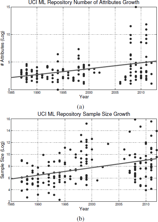
Plot (a) shows the dimensionality growth trend in the UCI Machine Learning Repository from the mid 1980s to 2012 while (b) shows the growth in the sample size for the same period.
However, these collected data are usually associated with a high level of noise. There are many reasons causing noise in these data, among which imperfection in the technologies that collected the data and the source of the data itself are two major reasons. For example, in the medical images domain, any deficiency in the imaging device will be reflected as noise for the later process. This kind of noise is caused by the device itself. The development of social media changes the role of online users from traditional content consumers to both content creators and consumers. The quality of social media data varies from excellent data to spam or abuse content by nature. Meanwhile, social media data are usually informally written and suffers from grammatical mistakes, misspelling, and improper punctuation. Undoubtedly, extracting useful knowledge and patterns from such huge and noisy data is a challenging task.
Dimensionality reduction is one of the most popular techniques to remove noisy (i.e., irrelevant) and redundant features. Dimensionality reduction techniques can be categorized mainly into feature extraction and feature selection. Feature extraction methods project features into a new feature space with lower dimensionality and the new constructed features are usually combinations of original features. Examples of feature extraction techniques include Principle Component Analysis (PCA), Linear Discriminant Analysis (LDA), and Canonical Correlation Analysis (CCA). On the other hand, the feature selection approaches aim to select a small subset of features that minimize redundancy and maximize relevance to the target such as the class labels in classification. Representative feature selection techniques include Information Gain, Relief, Fisher Score, and Lasso.
Both feature extraction and feature selection are capable of improving learning performance, lowering computational complexity, building better generalizable models, and decreasing required storage. Feature extraction maps the original feature space to a new feature space with lower dimensions by combining the original feature space. It is difficult to link the features from original feature space to new features. Therefore further analysis of new features is problematic since there is no physical meaning for the transformed features obtained from feature extraction techniques. Meanwhile, feature selection selects a subset of features from the original feature set without any transformation, and maintains the physical meanings of the original features. In this sense, feature selection is superior in terms of better readability and interpretability. This property has its significance in many practical applications such as finding relevant genes to a specific disease and building a sentiment lexicon for sentiment analysis. Typically feature selection and feature extraction are presented separately. Via sparse learning such as l1 regularization, feature extraction (transformation) methods can be converted into feature selection methods [48].
For the classification problem, feature selection aims to select subset of highly discriminant features. In other words, it selects features that are capable of discriminating samples that belong to different classes. For the problem of feature selection for classification, due to the availability of label information, the relevance of features is assessed as the capability of distinguishing different classes. For example, a feature fi is said to be relevant to a class cj if fi and cj are highly correlated.
In the following subsections, we will review the literature of data classification in Section (2.1.1), followed by general discussions about feature selection models in Section (2.1.2) and feature selection for classification in Section (2.1.3).
2.1.1 Data Classification
Classification is the problem of identifying to which of a set of categories (sub-populations) a new observation belongs, on the basis of a training set of data containing observations (or instances) whose category membership is known. Many real-world problems can be modeled as classification problems, such as assigning a given email into “spam” or “non-spam” classes, automatically assigning the categories (e.g., “Sports” and “Entertainment”) of coming news, and assigning a diagnosis to a given patient as described by observed characteristics of the patient (gender, blood pressure, presence or absence of certain symptoms, etc.). A general process of data classification is demonstrated in Figure 2.2, which usually consists of two phases — the training phase and the prediction phase.
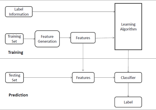
In the training phase, data is analyzed into a set of features based on the feature generation models such as the vector space model for text data. These features may either be categorical (e.g., “A”, “B”, “AB” or “O”, for blood type), ordinal (e.g., “large”, “medium”, or “small”), integer-valued (e.g., the number of occurrences of a part word in an email) or real-valued (e.g., a measurement of blood pressure). Some algorithms work only in terms of discrete data such as ID3 and require that real-valued or integer-valued data be discretized into groups (e.g., less than 5, between 5 and 10, or greater than 10). After representing data through these extracted features, the learning algorithm will utilize the label information as well as the data itself to learn a map function f (or a classifier) from features to labels, such as,
In the prediction phase, data is represented by the feature set extracted in the training process, and then the map function (or the classifier) learned from the training phase will perform on the feature represented data to predict the labels. Note that the feature set used in the training phase should be the same as that in the prediction phase.
There are many classification methods in the literature. These methods can be categorized broadly into linear classifiers, support vector machines, decision trees, and Neural networks. A linear classifier makes a classification decision based on the value of a linear combination of the features. Examples of linear classifiers include Fisher’s linear discriminant, logistic regression, the naive bayes classifier, and so on. Intuitively, a good separation is achieved by the hyperplane that has the largest distance to the nearest training data point of any class (so-called functional margin), since in general the larger the margin the lower the generalization error of the classifier. Therefore, the support vector machine constructs a hyperplane or set of hyperplanes by maximizing the margin. In decision trees, a tree can be learned by splitting the source set into subsets based on a feature value test. This process is repeated on each derived subset in a recursive manner called recursive partitioning. The recursion is completed when the subset at a node has all the same values of the target feature, or when splitting no longer adds value to the predictions.
2.1.2 Feature Selection
In the past thirty years, the dimensionality of the data involved in machine learning and data mining tasks has increased explosively. Data with extremely high dimensionality has presented serious challenges to existing learning methods [39], i.e., the curse of dimensionality [21]. With the presence of a large number of features, a learning model tends to overfit, resulting in the degeneration of performance. To address the problem of the curse of dimensionality, dimensionality reduction techniques have been studied, which is an important branch in the machine learning and data mining research area. Feature selection is a widely employed technique for reducing dimensionality among practitioners. It aims to choose a small subset of the relevant features from the original ones according to certain relevance evaluation criterion, which usually leads to better learning performance (e.g., higher learning accuracy for classification), lower computational cost, and better model interpretability.
According to whether the training set is labeled or not, feature selection algorithms can be categorized into supervised [61, 68], unsupervised [13, 51], and semi-supervised feature selection [11, 11]. Supervised feature selection methods can further be broadly categorized into filter models, wrapper models, and embedded models. The filter model separates feature selection from classifier learning so that the bias of a learning algorithm does not interact with the bias of a feature selection algorithm. It relies on measures of the general characteristics of the training data such as distance, consistency, dependency, information, and correlation. Relief [60], Fisher score [11], and Information Gain based methods [52] are among the most representative algorithms of the filter model. The wrapper model uses the predictive accuracy of a predetermined learning algorithm to determine the quality of selected features. These methods are prohibitively expensive to run for data with a large number of features. Due to these shortcomings in each model, the embedded model was proposed to bridge the gap between the filter and wrapper models. First, it incorporates the statistical criteria, as the filter model does, to select several candidate features subsets with a given cardinality. Second, it chooses the subset with the highest classification accuracy [40]. Thus, the embedded model usually achieves both comparable accuracy to the wrapper and comparable efficiency to the filter model. The embedded model performs feature selection in the learning time. In other words, it achieves model fitting and feature selection simultaneously [15, 54]. Many researchers also paid attention to developing unsupervised feature selection. Unsupervised feature selection is a less constrained search problem without class labels, depending on clustering quality measures [12], and can eventuate many equally valid feature subsets. With high-dimensional data, it is unlikely to recover the relevant features without considering additional constraints. Another key difficulty is how to objectively measure the results of feature selection [12]. A comprehensive review about unsupervised feature selection can be found in [1]. Supervised feature selection assesses the relevance of features guided by the label information but a good selector needs enough labeled data, which is time consuming. While unsupervised feature selection works with unlabeled data, it is difficult to evaluate the relevance of features. It is common to have a data set with huge dimensionality but small labeled-sample size. High-dimensional data with small labeled samples permits too large a hypothesis space yet with too few constraints (labeled instances). The combination of the two data characteristics manifests a new research challenge. Under the assumption that labeled and unlabeled data are sampled from the same population generated by target concept, semi-supervised feature selection makes use of both labeled and unlabeled data to estimate feature relevance [11].
Feature weighting is thought of as a generalization of feature selection [69]. In feature selection, a feature is assigned a binary weight, where 1 means the feature is selected and 0 otherwise. However, feature weighting assigns a value, usually in the interval [0,1] or [-1,1], to each feature. The greater this value is, the more salient the feature will be. Most of the feature weight algorithms assign a unified (global) weight to each feature over all instances. However, the relative importance, relevance, and noise in the different dimensions may vary significantly with data locality. There are local feature selection algorithms where the local selection of features is done specific to a test instance, which is is common in lazy leaning algorithms such as kNN [9, 22]. The idea is that feature selection or weighting is done at classification time (rather than at training time), because knowledge of the test instance sharpens the ability to select features.
Typically, a feature selection method consists of four basic steps [40], namely, subset generation, subset evaluation, stopping criterion, and result validation. In the first step, a candidate feature subset will be chosen based on a given search strategy, which is sent, in the second step, to be evaluated according to a certain evaluation criterion. The subset that best fits the evaluation criterion will be chosen from all the candidates that have been evaluated after the stopping criterion are met. In the final step, the chosen subset will be validated using domain knowledge or a validation set.
2.1.3 Feature Selection for Classification
The majority of real-world classification problems require supervised learning where the underlying class probabilities and class-conditional probabilities are unknown, and each instance is associated with a class label [8]. In real-world situations, we often have little knowledge about relevant features. Therefore, to better represent the domain, many candidate features are introduced, resulting in the existence of irrelevant/redundant features to the target concept. A relevant feature is neither irrelevant nor redundant to the target concept; an irrelevant feature is not directly associated with the target concept but affects the learning process, and a redundant feature does not add anything new to the target concept [8]. In many classification problems, it is difficult to learn good classifiers before removing these unwanted features due to the huge size of the data. Reducing the number of irrelevant/redundant features can drastically reduce the running time of the learning algorithms and yields a more general classifier. This helps in getting a better insight into the underlying concept of a real-world classification problem.
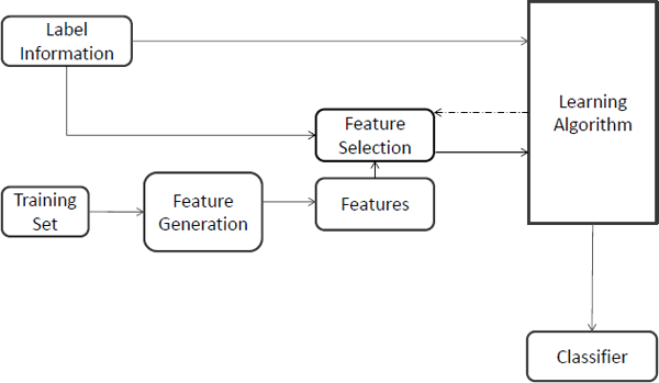
A general feature selection for classification framework is demonstrated in Figure 2.3. Feature selection mainly affects the training phase of classification. After generating features, instead of processing data with the whole features to the learning algorithm directly, feature selection for classification will first perform feature selection to select a subset of features and then process the data with the selected features to the learning algorithm. The feature selection phase might be independent of the learning algorithm, as in filter models, or it may iteratively utilize the performance of the learning algorithms to evaluate the quality of the selected features, as in wrapper models. With the finally selected features, a classifier is induced for the prediction phase.
Usually feature selection for classification attempts to select the minimally sized subset of features according to the following criteria:
- the classification accuracy does not significantly decrease; and
- the resulting class distribution, given only the values for the selected features, is as close as possible to the original class distribution, given all features.
Ideally, feature selection methods search through the subsets of features and try to find the best one among the competing 2m candidate subsets according to some evaluation functions [8]. However, this procedure is exhaustive as it tries to find only the best one. It may be too costly and practically prohibitive, even for a medium-sized feature set size (m). Other methods based on heuristic or random search methods attempt to reduce computational complexity by compromising performance. These methods need a stopping criterion to prevent an exhaustive search of subsets.
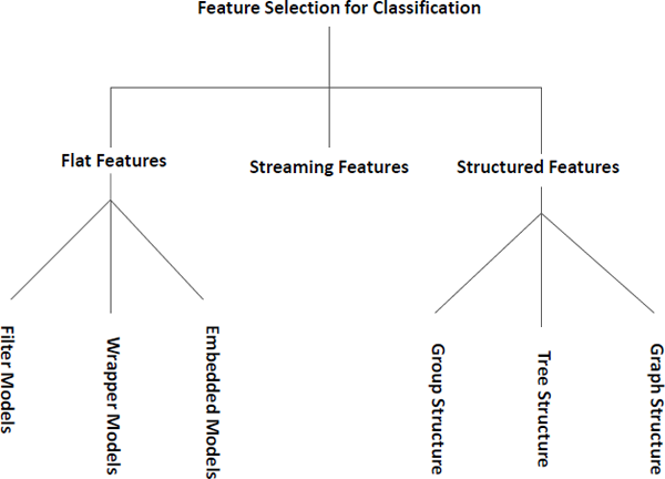
In this chapter, we divide feature selection for classification into three families according to the feature structure — methods for flat features, methods for structured features, and methods for streaming features as demonstrated in Figure 2.4. In the following sections, we will review these three groups with representative algorithms in detail.
Before going to the next sections, we introduce notations we adopt in this book chapter. Assume that F={f1,f2,…,fm}andC={c1,c2,…,cK} denote the feature set and the class label set where m and K are the numbers of features and labels, respectively. X={x1,x2,…,x3}∈ℝm×n is the data where n is the number of instances and the label information of the i-th instance xi is denoted as yi.
2.2 Algorithms for Flat Features
In this section, we will review algorithms for flat features, where features are assumed to be independent. Algorithms in this category are usually further divided into three groups — filter models, wrapper models, and embedded models.
2.2.1 Filter Models
Relying on the characteristics of data, filter models evaluate features without utilizing any classification algorithms [39]. A typical filter algorithm consists of two steps. In the first step, it ranks features based on certain criteria. Feature evaluation could be either univariate or multivariate. In the univariate scheme, each feature is ranked independently of the feature space, while the multivariate scheme evaluates features in an batch way. Therefore, the multivariate scheme is naturally capable of handling redundant features. In the second step, the features with highest rankings are chosen to induce classification models. In the past decade, a number of performance criteria have been proposed for filter-based feature selection, such as Fisher score [10], methods based on mutual information [37, 52, 74], and ReliefF and its variants [34, 56].
Fisher Score [10]: Features with high quality should assign similar values to instances in the same class and different values to instances from different classes. With this intuition, the score for the i-th feature Si will be calculated by Fisher Score as,
Si=ΣKk=1nj(μij−μi)2ΣKk=1njρ2ij,(2.2)
where μij and ρij are the mean and the variance of the i-th feature in the j-th class, respectively, nj is the number of instances in the j-th class, and μi is the mean of the i-th feature.
Fisher Score evaluates features individually; therefore, it cannot handle feature redundancy. Recently, Gu et al. [17] proposed a generalized Fisher score to jointly select features, which aims to find a subset of features that maximize the lower bound of traditional Fisher score and solve the following problem:
||W⊤diag(p)X−G||2F+γ||W||2F,s.t.,p∈{0,1}m,p⊤1=d,(2.3)
where p is the feature selection vector, d is the number of features to select, and G is a special label indicator matrix, as follows:
G(i,j)={√nnj−√njn if xi∈cj,−√njn otherwise.(2.4)
Mutual Information based on Methods [37, 52, 74]: Due to its computational efficiency and simple interpretation, information gain is one of the most popular feature selection methods. It is used to measure the dependence between features and labels and calculates the information gain between the i-th feature fi and the class labels C as
IG(fi,C)=H(fi)−H(fi|C),(2.5)
where H(fi) is the entropy of fi and H(fi|C) is the entropy of fi after observing C:
H(fi)=−∑jp(xj)log2(p(xj)),H(fi|C)=−∑kp(ck)∑jp(xj|ck)log2(p(xj|ck)).(2.6)
In information gain, a feature is relevant if it has a high information gain. Features are selected in a univariate way, therefore, information gain cannot handle redundant features. In [74], a fast filter method FCBF based on mutual information was proposed to identify relevant features as well as redundancy among relevant features and measure feature-class and feature-feature correlation. Given a threshold ρ, FCBC first selects a set of features S that is highly correlated to the class with SU ≥ ρ, where SU is symmetrical uncertainty defined as
SU(fi,C)=2IG(fi,C)H(fi)+H(C).(2.7)
A feature fi is called predominant iff SU (fi,ck)≥ρ and there is no fj(fj∈S,j≠i) such as SU(j,i)≥SU(i,ck). fj is a redundant feature to fi if SU(j,i)≥SU(i,ck). Then the set of redundant features is denoted as S(Pi), which is further split into S+pi and S−pi. S+pi and S−pi contain redundant features to fi with SU(j,ck)>SU(i,ck) and SU(j,ck)≤SU(i,ck), respectively. Finally FCBC applied three heuristics on S(Pi),S+pi and S−pi to remove the redundant features and keep the features that are most relevant to the class. FCBC provides an effective way to handle feature redundancy in feature selection.
Minimum-Redundancy-Maximum-Relevance (mRmR) is also a mutual information based method and it selects features according to the maximal statistical dependency criterion [52]. Due to the difficulty in directly implementing the maximal dependency condition, mRmR is an approximation to maximizing the dependency between the joint distribution of the selected features and the classification variable. Minimize Redundancy for discrete features and continuous features is defined as:
for Discrete Features: minWI, WI=1|S|2∑i,j∈SI(i,j),for Continuous Features: minWC, WC=1|S|2∑i,j∈S|C(i,j)|(2.8)
where I(i, j) and C(i, j) are mutual information and the correlation between fi and fj, respectively. Meanwhile, Maximize Relevance for discrete features and continuous features is defined as:
for Discrete Features: maxVI, VI=1|S|2∑i∈SI(h,i),for Continuous Features: maxVC, VC=1|S|2∑iF(i,h)(2.9)
where h is the target class and F(i, h) is the F-statistic.
ReliefF [34, 56]: Relief and its multi-class extension ReliefF select features to separate instances from different classes. Assume that l instances are randomly sampled from the data and then the score of the i-th feature Si is defined by Relief as,
Si=12l∑k=1d(Xik−XiMk)−d(Xik−XiHk),(2.10)
where Mk denotes the values on the i-th feature of the nearest instances to xk with the same class label, while Hk denotes the values on the i-th feature of the nearest instances to xk with different class labels. d(⋅) is a distance measure. To handle multi-class problem, Equation (2.10) is extended as,
Si=1Kl∑k=1(−1mk∑xj∈Mkd(Xik−Xij)+∑y≠yk1hkyp(y)1−p(y)∑xj∈Hkd(Xik−Xij))(2.11)
where Mk and Hky denotes the sets of nearest points to xk with the same class and the class y with sizes of mk and hky respectively, and p(y) is the probability of an instance from the class y. In [56], the authors related the relevance evaluation criterion of ReliefF to the hypothesis of margin maximization, which explains why the algorithm provides superior performance in many applications.
2.2.2 Wrapper Models
Filter models select features independent of any specific classifiers. However the major disadvantage of the filter approach is that it totally ignores the effects of the selected feature subset on the performance of the induction algorithm [20, 36]. The optimal feature subset should depend on the specific biases and heuristics of the induction algorithm. Based on this assumption, wrapper models utilize a specific classifier to evaluate the quality of selected features, and offer a simple and powerful way to address the problem of feature selection, regardless of the chosen learning machine [26, 36]. Given a predefined classifier, a typical wrapper model will perform the following steps:
- Step 1: searching a subset of features,
- Step 2: evaluating the selected subset of features by the performance of the classifier,
- Step 3: repeating Step 1 and Step 2 until the desired quality is reached.
A general framework for wrapper methods of feature selection for classification [36] is shown in Figure 2.5, and it contains three major components:
- feature selection search — how to search the subset of features from all possible feature subsets,
- feature evaluation — how to evaluate the performance of the chosen classifier, and
- induction algorithm.
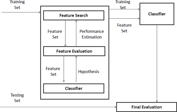
In wrapper models, the predefined classifier works as a black box. The feature search component will produce a set of features and the feature evaluation component will use the classifier to estimate the performance, which will be returned back to the feature search component for the next iteration of feature subset selection. The feature set with the highest estimated value will be chosen as the final set to learn the classifier. The resulting classifier is then evaluated on an independent testing set that is not used during the training process [36].
The size of search space for m features is O(2m), thus an exhaustive search is impractical unless m is small. Actually the problem is known to be NP-hard [18]. A wide range of search strategies can be used, including hill-climbing, best-first, branch-and-bound, and genetic algorithms [18]. The hill-climbing strategy expands the current set and moves to the subset with the highest accuracy, terminating when no subset improves over the current set. The best-first strategy is to select the most promising set that has not already been expanded and is a more robust method than hill- climbing [36]. Greedy search strategies seem to be particularly computationally advantageous and robust against overfitting. They come in two flavors — forward selection and backward elimination. Forward selection refers to a search that begins at the empty set of features and features are progressively incorporated into larger and larger subsets, whereas backward elimination begins with the full set of features and progressively eliminates the least promising ones. The search component aims to find a subset of features with the highest evaluation, using a heuristic function to guide it. Since we do not know the actual accuracy of the classifier, we use accuracy estimation as both the heuristic function and the valuation function in the feature evaluation phase. Performance assessments are usually done using a validation set or by cross-validation.
Wrapper models obtain better predictive accuracy estimates than filter models [36, 38]. However, wrapper models are very computationally expensive compared to filter models. It produces better performance for the predefined classifier since we aim to select features that maximize the quality; therefore the selected subset of features is inevitably biased to the predefined classifier.
2.2.3 Embedded Models
Filter models select features that are independent of the classifier and avoid the cross-validation step in a typical wrapper model; therefore they are computationally efficient. However, they do not take into account the biases of the classifiers. For example, the relevance measure of Relief would not be appropriate as feature subset selectors for Naive-Bayes because in many cases the performance of Naive-Bayes improves with the removal of relevant features [18]. Wrapper models utilize a predefined classifier to evaluate the quality of features and representational biases of the classifier are avoided by the feature selection process. However, they have to run the classifier many times to assess the quality of selected subsets of features, which is very computationally expensive. Embedded Models embedding feature selection with classifier construction, have the advantages of (1) wrapper models — they include the interaction with the classification model and (2) filter models — and they are far less computationally intensive than wrapper methods [40, 46, 57].
There are three types of embedded methods. The first are pruning methods that first utilize all features to train a model and then attempt to eliminate some features by setting the corresponding coefficients to 0, while maintaining model performance such as recursive feature elimination using a support vector machine (SVM) [5, 19]. The second are models with a built-in mechanism for feature selection such as ID3 [55] and C4.5 [54]. The third are regularization models with objective functions that minimize fitting errors and in the meantime force the coefficients to be small or to be exactly zero. Features with coefficients that are close to 0 are then eliminated [46]. Due to good performance, regularization models attract increasing attention. We will review some representative methods below based on a survey paper of embedded models based on regularization [46].
Without loss of generality, in this section, we only consider linear classifiers w in which classification of Y can be based on a linear combination of X such as SVM and logistic regression. In regularization methods, classifier induction and feature selection are achieved simultaneously by estimating w with properly tuned penalties. The learned classifier w can have coefficients exactly equal to zero. Since each coefficient of w corresponds to one feature such as wi for fi, feature selection is achieved and only features with nonzero coefficients in w will be used in the classifier.
Specifically, we define ˆw as,
ˆw=minwc(w,X)+α penalty(w)(2.12)
where c(⋅) is the classification objective function, penalty(w) is a regularization term, and α is the regularization parameter controlling the trade-off between the c(⋅) and the penalty. Popular choices of c(⋅) include quadratic loss such as least squares, hinge loss such as l1SVM [5], and logistic loss such as BlogReg [15].
Quadratic loss:
c(w,X)=n∑i=1(yi−w⊤xi)2,(2.13)
Hinge loss:
c(w,X)=n∑i=1max(0,1−yiw⊤xi),(2.14)
Logistic loss:
c(w,X)=n∑i=1log(1+exp(−yi(w⊤xi+b))).(2.15)
Lasso Regularization [64]: Lasso regularization is based on l1-norm of the coefficient of w and defined as
penalty(w)=m∑i=1|wi|.(2.16)
An important property of the l1 regularization is that it can generate an estimation of w [64] with exact zero coefficients. In other words, there are zero entities in w, which denotes that the corresponding features are eliminated during the classifier learning process. Therefore, it can be used for feature selection.
Adaptive Lasso [80]: The Lasso feature selection is consistent if the underlying model satisfies a non-trivial condition, which may not be satisfied in practice [76]. Meanwhile the Lasso shrinkage produces biased estimates for the large coefficients; thus, it could be suboptimal in terms of estimation risk [14].
The adaptive Lasso is proposed to improve the performance of as [80]
penalty(w)=m∑i=11bi|wi|,(2.17)
where the only difference between Lasso and adaptive Lasso is that the latter employs a weighted adjustment bi for each coefficient wi. The article shows that the adaptive Lasso enjoys the oracle properties and can be solved by the same efficient algorithm for solving the Lasso.
The article also proves that for linear models w with n ≫ m, the adaptive Lasso estimate is selection consistent under very general conditions if bi is a √n consistent estimate of wi. Complimentary to this proof, [24] shows that when m ≫ n for linear models, the adaptive Lasso estimate is also selection consistent under a partial orthogonality condition in which the covariates with zero coefficients are weakly correlated with the covariates with nonzero coefficients.
Bridge regularization [23, 35]: Bridge regularization is formally defined as
penalty(w)=n∑i=1|wi|γ,0≤γ≤1.(2.18)
Lasso regularization is a special case of bridge regularization when γ = 1.
For linear models, the bridge regularization is feature selection consistent, even when the Lasso is not [23] when n ≫ m and γ < 1; the regularization is still feature selection consistent if the features associated with the phenotype and those not associated with the phenotype are only weakly correlated when n ≫ m and γ < 1.
Elastic net regularization [81]: In practice, it is common that a few features are highly correlated. In this situation, the Lasso tends to select only one of the correlated features [81]. To handle features with high correlations, elastic net regularization is proposed as
penalty(w)=n∑i=1|wi|γ+(n∑i=1w2i)λ,(2.19)
with 0 < γ < 1 and λ ≥ 1. The elastic net is a mixture of bridge regularization with different values of γ. [81] proposes γ = 1 and γ = 1, which is extended to γ < 1 and γ = 1 by [43].
Through the loss function c(w, X), the above-mentioned methods control the size of residuals. An alternative way to obtain a sparse estimation of w is Dantzig selector, which is based on the normal score equations and controls the correlation of residuals with X as [6],
min||w||1,s.t. ||X⊤(y−w⊤X)||∞≤λ,(2.20)
∥⋅∥∞ is the l∞-norm of a vector and Dantzig selector was designed for linear regression models. Candes and Tao have provided strong theoretical justification for this performance by establishing sharp non-asymptotic bounds on the l2-error in the estimated coefficients, and showed that the error is within a factor of log(p) of the error that would be achieved if the locations of the non-zero coefficients were known [6, 28]. Strong theoretical results show that LASSO and Dantzig selector are closely related [28].
2.3 Algorithms for Structured Features
The models introduced in the last section assume that features are independent and totally overlook the feature structures [73]. However, for many real-world applications, the features exhibit certain intrinsic structures, e.g., spatial or temporal smoothness [65, 79], disjoint/overlapping groups [29], trees [33], and graphs [25]. Incorporating knowledge about the structures of features may significantly improve the classification performance and help identify the important features. For example, in the study of arrayCGH [65, 66], the features (the DNA copy numbers along the genome) have the natural spatial order, and incorporating the structure information using an extension of the l1-norm outperforms the Lasso in both classification and feature selection. In this section, we review feature selection algorithms for structured features and these structures include group, tree, and graph.
Since most existing algorithms in this category are based on linear classifiers, we focus on linear classifiers such as SVM and logistic classifiers in this section. A very popular and successful approach to learn linear classifiers with structured features is to minimize a empirical error penalized by a regularization term as
minw c(w⊤X,Y)+α penalty(w,G),(2.21)
where G denotes the structure of features, and α controls the trade-off between data fitting and regularization. Equation (2.21) will lead to sparse classifiers, which lend themselves particularly well to interpretation, which is often of primary importance in many applications such as biology or social sciences [75].
2.3.1 Features with Group Structure
In many real-world applications, features form group structures. For example, in the multifactor analysis-of-variance (ANOVA) problem, each factor may have several levels and can be denoted as a group of dummy features [75]; in speed and signal processing, different frequency bands can be represented by groups [49]. When performing feature selection, we tend to select or not select features in the same group simultaneously. Group Lasso, driving all coefficients in one group to zero together and thus resulting in group selection, attracts more and more attention [3, 27, 41, 50, 75].
Assume that features form k disjoint groups G = {G1, G2, …, Gk} and there is no overlap between any two groups. With the group structure, we can rewrite w into the block form as w = {w1, w2, …, wk} where wi corresponds to the vector of all coefficients of features in the i-th group Gi. Then, the group Lasso performs the lq,1-norm regularization on the model parameters as
penalty(w,G)=k∑i=1hi||wGi||q,(2.22)
where ∥⋅∥q is the lq-norm with q > 1, and hi is the weight for the i-th group. Lasso does not take group structure information into account and does not support group selection, while group Lasso can select or not select a group of features as a whole.
Once a group is selected by the group Lasso, all features in the group will be selected. For certain applications, it is also desirable to select features from the selected groups, i.e., performing simultaneous group selection and feature selection. The sparse group Lasso takes advantages of both Lasso and group Lasso, and it produces a solution with simultaneous between- and within-group sparsity. The sparse group Lasso regularization is based on a composition of the lq,1-norm and the l1-norm,
penalty(w,G)=α||w||1+(1−α)k∑i=1hi||wGi||q,(2.23)
where α ∈ [0,1], the first term controls the sparsity in the feature level, and the second term controls the group selection.
Figure 2.6 demonstrates the different solutions among Lasso, group Lasso, and sparse group Lasso. In the figure, features form four groups {G1, G2, G3, G4}. Light color denotes the corresponding feature of the cell with zero coefficients and dark color indicates non-zero coefficients. From the figure, we observe that
- Lasso does not consider the group structure and selects a subset of features among all groups;
- group Lasso can perform group selection and select a subset of groups. Once the group is selected, all features in this group are selected; and
- sparse group Lasso can select groups and features in the selected groups at the same time.
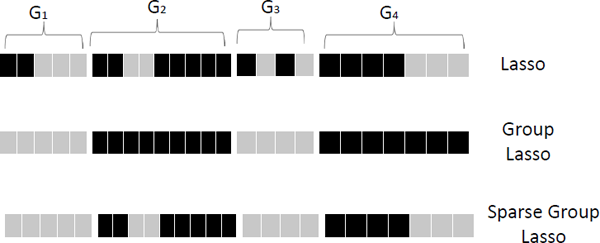
Illustration of Lasso, group Lasso and sparse group Lasso. Features can be grouped into four disjoint groups {G1, G2, G3, G4}. Each cell denotes a feature and light color represents the corresponding cell with coefficient zero.
In some applications, the groups overlap. One motivation example is the use of biologically meaningful gene/protein sets (groups) given by [73]. If the proteins/genes either appear in the same pathway, or are semantically related in terms of gene ontology (GO) hierarchy, or are related from gene set enrichment analysis (GSEA), they are related and assigned to the same groups. For example, the canonical pathway in MSigDB has provided 639 groups of genes. It has been shown that the group (of proteins/genes) markers are more reproducible than individual protein/gene markers and modeling such group information as prior knowledge can improve classification performance [7]. Groups may overlap — one protein/gene may belong to multiple groups. In these situations, group Lasso does not correctly handle overlapping groups and a given coefficient only belongs to one group. Algorithms investigating overlapping groups are proposed as [27, 30, 33, 42]. A general overlapping group Lasso regularization is similar to that for group Lasso regularization in Equation (2.23)
penalty(w,G)=α||w||1+(1−α)k∑i=1hi||wGi||q,(2.24)
however, groups for overlapping group Lasso regularization may overlap, while groups in group Lasso are disjoint.
2.3.2 Features with Tree Structure
In many applications, features can naturally be represented using certain tree structures. For example, the image pixels of the face image can be represented as a tree, where each parent node contains a series of child nodes that enjoy spatial locality; genes/proteins may form certain hierarchical tree structures [42]. Tree-guided group Lasso regularization is proposed for features represented as an index tree [30, 33, 42].
In the index tree, each leaf node represents a feature and each internal node denotes the group of the features that correspond to the leaf nodes of the subtree rooted at the given internal node. Each internal node in the tree is associated with a weight that represents the height of the subtree, or how tightly the features in the group for that internal node are correlated, which can be formally defined as follows [42].
For an index tree G of depth d, let Gi={Gi1,Gi2,…,Gini} contain all the nodes corresponding to depth i where ni is the number of nodes of the depth i. The nodes satisfy the following conditions:
- the nodes from the same depth level have non-overlapping indices, i.e., Gij∩Gik=0, ∀i∈{1,2,…,d}, j≠k, 1≤j,k≤ni;
- let Gi−1j0 be the parent node of a non-root node Gij, then Gij⊆Gi−1j0.
Figure 2.7 shows a sample index tree of depth 3 with 8 features, where Gij are defined as
G01={f1,f2,f3,f4,f5,f6,f7,f8},G11={f1,f2},G21={f3,f4,f5,f6f7},G31={f8},G21={f1,f2},G22={f3,f4}G32={f5,f6,f7}.
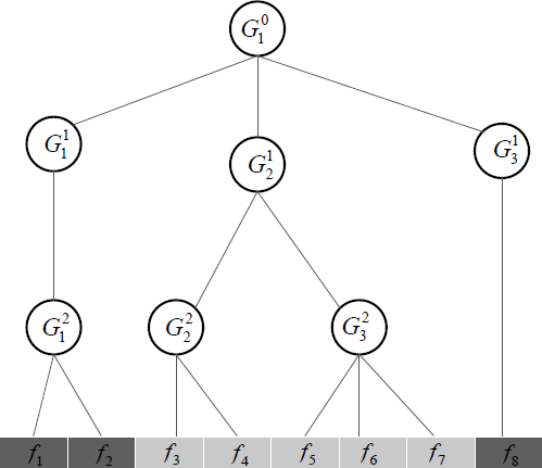
We can observe that
- G01 contains all features;
- the index sets from different nodes may overlap, e.g., any parent node overlaps with its child nodes;
- the nodes from the same depth level do not overlap; and
- the index set of a child node is a subset of that of its parent node.
With the definition of the index tree, the tree-guided group Lasso regularization is,
penalty(w,G)=d∑i=0ni∑j=1hij||wGij||q,(2.25)
Since any parent node overlaps with its child nodes, if a specific node is not selected (i.e., its corresponding model coefficient is zero), then all its child nodes will not be selected. For example, in Figure 2.7, if G12 is not selected, both G22 and G23 will not be selected, indicating that features {f3, f4, f5, f6, f7} will be not selected. Note that the tree structured group Lasso is a special case of the overlapping group Lasso with a specific tree structure.
2.3.3 Features with Graph Structure
We often have knowledge about pair-wise dependencies between features in many real-world applications [58]. For example, in natural language processing, digital lexicons such as WordNet can indicate which words are synonyms or antonyms; many biological studies have suggested that genes tend to work in groups according to their biological functions, and there are some regulatory relationships between genes. In these cases, features form an undirected graph, where the nodes represent the features, and the edges imply the relationships between features. Several recent studies have shown that the estimation accuracy can be improved using dependency information encoded as a graph.
Let G(N,E) be a given graph where N = {1,2, …,m} is a set of nodes, and E is a set of edges. Node i corresponds to the i-th feature and we use A ∈ ℝm×m to denote the adjacency matrix of G. Figure 2.8 shows an example of the graph of 7 features {f1, f2, …,f7} and its representation A.
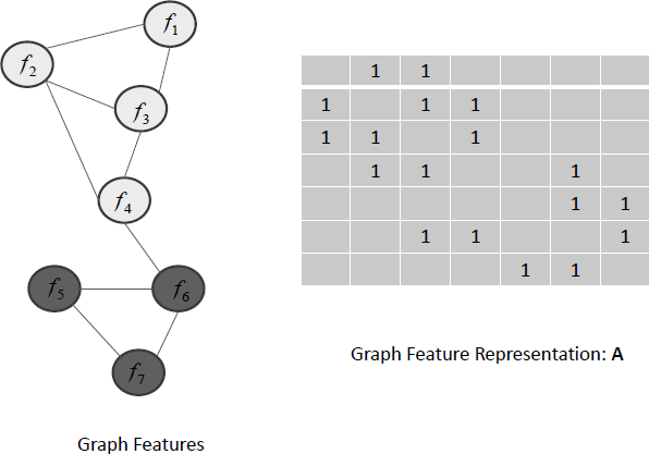
An illustration of the graph of 7 features {f1, f2, ..., f7} and its corresponding representation A.
If nodes i and j are connected by an edge in E, then the i-th feature and the j-th feature are more likely to be selected together, and they should have similar weights. One intuitive way to formulate graph Lasso is to force weights of two connected features close by a squre loss as
penalty(w,G)=λ||w||1+(1−λ)∑i,jAij(wi−wj)2,(2.26)
which is equivalent to
penalty(w,G)=λ||w||1+(1−λ)w⊤ℒw,(2.27)
where L = D — A is the Laplacian matrix and D is a diagonal matrix with Dii=∑mj=1Aij. The Laplacian matrix is positive semi-definite and captures the underlying local geometric structure of the data. When L is an identity matrix, w⊤ℒw=||w||22 and then Equation (2.27) reduces to the elastic net penalty [81]. Because w⊤ℒw is both convex and differentiable, existing efficient algorithms for solving the Lasso can be applied to solve Equation (2.27).
Equation (2.27) assumes that the feature graph is unsigned, and encourages positive correlation between the values of coefficients for the features connected by an edge in the unsigned graph. However, two features might be negatively correlated. In this situation, the feature graph is signed, with both positive and negative edges. To perform feature selection with a signed feature graph, GFlasso employs a different l1 regularization over a graph [32],
penalty(w,G)=λ||w||1+(1−λ)∑i,jAij||wi−sign(rij)xj||,(2.28)
where rij is the correlation between two features. When fi and fj are positively connected, rij > 0, i.e., with a positive edge, penalty(w,G) forces the coefficients wi and wj to be similar; while fi and fj are negatively connected, rij > 0, i.e., with a negative edge, the penalty forces wi and wj to be dissimilar. Due to possible graph misspecification, GFlasso may introduce additional estimation bias in the learning process. For example, additional bias may occur when the sign of the edge between fi and fj is inaccurately estimated.
In [72], the authors introduced several alternative formulations for graph Lasso. One of the formulations is defined as
penalty(w,G)=λ||w||1+(1−λ)∑i,jAijmax(|wi|,|wj|),(2.29)
where a pairwise l∞ regularization is used to force the coefficients to be equal and the grouping constraints are only put on connected nodes with Aij = 1. The l1 -norm of w encourages sparseness, and max (|wi|, |wj|) will penalize the larger coefficients, which can be decomposed as
max(|wi|,|wj|)=12(|wi+wj|+|wi−wj|),(2.30)
which can be further represented as
max(|wi|,|wj|)=|u⊤w|+|v⊤w|,(2.31)
where u and v are two vectors with only two non-zero entities, i.e., ui=uj=12 and vi=−vj=12.
The GOSCAR formulation is closely related to OSCAR in [4]. However, OSCAR assumes that all features form a complete graph, which means that the feature graph is complete. OSCAR works for A whose entities are all 1, while GOSCAR can work with an arbitrary undirected graph where A is any symmetric matrix. In this sense, GOSCAR is more general. Meanwhile, the formulation for GOSCAR is much more challenging to solve than that of OSCAR.
The limitation of the Laplacian Lasso — that the different signs of coefficients can introduce additional penalty — can be overcome by the grouping penalty of GOSCAR. However, GOSCAR can easily overpenalize the coefficient wi or wj due to the property of the max operator. The additional penalty would result in biased estimation, especially for large coefficients. As mentioned above, GFlasso will introduce estimation bias when the sign between wi and wj is wrongly estimated. This motivates the following non-convex formulation for graph features,
penalty(w,G)=λ||w||1+(1−λ)∑i,jAij|||wi|−|wj|||,(2.32)
where the grouping penalty ∑i,jAij|||wi|−|wj||| controls only magnitudes of differences of coefficients while ignoring their signs over the graph. Via the l1 regularization and grouping penalty, feature grouping and selection are performed simultaneously where only large coefficients as well as pairwise difference are shrunk [72].
For features with graph structure, a subset of highly connected features in the graph is likely to be selected or not selected as a whole. For example, in Figure 2.8, {f5, f6, f7} are selected, while {f1, f2, f3, f4} are not selected.
2.4 Algorithms for Streaming Features
Methods introduced above assume that all features are known in advance, and another interesting scenario is taken into account where candidate features are sequentially presented to the classifier for potential inclusion in the model [53, 67, 70, 78]. In this scenario, the candidate features are generated dynamically and the size of features is unknown. We call this kind of features streaming features and feature selection for streaming features is called streaming feature selection. Streaming feature selection has practical significance in many applications. For example, the famous microblogging Web site Twitter produces more than 250 millions tweets per day and many new words (features) are generated, such as abbreviations. When performing feature selection for tweets, it is not practical to wait until all features have been generated, thus it could be more preferable to streaming feature selection.
A general framework for streaming feature selection is presented in Figure 2.9. A typical streaming feature selection will perform the following steps:
- Step 1: Generating a new feature.
- Step 2: Determining whether to add the newly generated feature to the set of currently selected features.
- Step 3: Determining whether to remove features from the set of currently selected features.
- Step 4: Repeat Step 1 to Step 3.
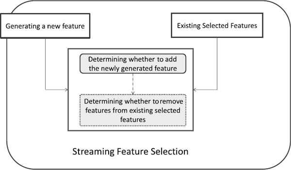
Different algorithms may have different implementations for Step 2 and Step 3, and next we will review some representative methods in this category. Note that Step 3 is optional and some streaming feature selection algorithms only implement Step 2.
2.4.1 The Grafting Algorithm
Perkins and Theiler proposed a streaming feature selection framework based on grafting, which is a general technique that can be applied to a variety of models that are parameterized by a weight vector w, subject to l1 regularization, such as the Lasso regularized feature selection framework in Section 2.2.3, as
ˆw=minwc(w,X)+αm∑j=1|wj|.(2.33)
When all features are available, penalty(w) penalizes all weights in w uniformly to achieve feature selection, which can be applied to streaming features with the grafting technique. In Equation (2.33), every one-zero weight wj added to the model incurs a regularize penalty of α|wj|. Therefore the feature adding to the model only happens when the loss of c(⋅) is larger than the regularizer penalty. The grafting technique will only take wj away from zero if:
∂c∂wj>α,(2.34)
otherwise the grafting technique will set the weight to zero (or exclude the feature).
2.4.2 The Alpha-Investing Algorithm
α-investing controls the false discovery rate by dynamically adjusting a threshold on the p-statistic for a new feature to enter the model [78], which is described as
- Initialize w0, i = 0, selected features in the model SF = 0
- Step 1: Get a new feature fi
- Step 2: Set αi = wi/(2i)
- Step 3:
wi+1=wi−αiif pvalue(xi,SF)≥αi.wi+1=wi+α△−αi, SF=SF∪fi otherwise
- Step 4: i = i+1
- Step 5: Repeat Step 1 to Step 3
where the threshold αi is the probability of selecting a spurious feature in the i-th step and it is adjusted using the wealth wi, which denotes the current acceptable number of future false positives. Wealth is increased when a feature is selected to the model, while wealth is decreased when a feature is not selected to the model. The p-value is the probability that a feature coefficient could be judged to be non-zero when it is actually zero, which is calculated by using the fact that Δ-Loglikelihood is equivalent to t-statistics. The idea of α-investing is to adaptively control the threshold for selecting features so that when new features are selected to the model, one “invests” α increasing the wealth raising the threshold, and allowing a slightly higher future chance of incorrect inclusion of features. Each time a feature is tested and found not to be significant, wealth is “spent,” reducing the threshold so as to keep the guarantee of not selecting more than a target fraction of spurious features.
2.4.3 The Online Streaming Feature Selection Algorithm
To determine the value of α, the grafting algorithm requires all candidate features in advance, while the α-investing algorithm needs some prior knowledge about the structure of the feature space to heuristically control the choice of candidate feature selection, and it is difficult to obtain sufficient prior information about the structure of the candidate features with a feature stream. Therefore the online streaming feature selection algorithm (OSFS) is proposed to solve these challenging issues in streaming feature selection [70].
An entire feature set can be divided into four basic disjoint subsets — (1) irrelevant features, (2) redundant feature, (3) weakly relevant but non-redundant features, and (4) strongly relevant features. An optimal feature selection algorithm should have non-redundant and strongly relevant features. For streaming features, it is difficult to find all strongly relevant and non-redundant features. OSFS finds an optimal subset using a two-phase scheme — online relevance analysis and redundancy analysis. A general framework of OSFS is presented as follows:
- Initialize BCF = ;
- Step 1: Generate a new feature fk;
- Step 2: Online relevance analysis
Disregard fk, if fk is irrelevant to the class labels.
BCF = BCF ⋃ fk otherwise;
- Step 3: Online Redundancy Analysis;
- Step 4: Alternate Step 1 to Step 3 until the stopping criteria are satisfied.
In the relevance analysis phase, OSFS discovers strongly and weakly relevant features, and adds them into best candidate features (BCF). If a new coming feature is irrelevant to the class label, it is discarded, otherwise it is added to BCF.
In the redundancy analysis, OSFS dynamically eliminates redundant features in the selected subset. For each feature fk in BCF, if there exists a subset within BCF making fk and the class label conditionally independent, fk is removed from BCF. An alternative way to improve the efficiency is to further divide this phase into two analyses — inner-redundancy analysis and outer-redundancy analysis. In the inner-redundancy analysis, OSFS only re-examines the feature newly added into BCF, while the outer-redundancy analysis re-examines each feature of BCF only when the process of generating a feature is stopped.
2.5 Discussions and Challenges
Here are several challenges and concerns that we need to mention and discuss briefly in this chapter about feature selection for classification.
2.5.1 Scalability
With the tremendous growth of dataset sizes, the scalability of current algorithms may be in jeopardy, especially with these domains that require an online classifier. For example, data that cannot be loaded into the memory require a single data scan where the second pass is either unavailable or very expensive. Using feature selection methods for classification may reduce the issue of scalability for clustering. However, some of the current methods that involve feature selection in the classification process require keeping full dimensionality in the memory. Furthermore, other methods require an iterative process where each sample is visited more than once until convergence.
On the other hand, the scalability of feature selection algorithms is a big problem. Usually, they require a sufficient number of samples to obtain, statically, adequate results. It is very hard to observe feature relevance score without considering the density around each sample. Some methods try to overcome this issue by memorizing only samples that are important or a summary. In conclusion, we believe that the scalability of classification and feature selection methods should be given more attention to keep pace with the growth and fast streaming of the data.
2.5.2 Stability
Algorithms of feature selection for classification are often evaluated through classification accuracy. However, the stability of algorithms is also an important consideration when developing feature selection methods. A motivated example is from bioinformatics: The domain experts would like to see the same or at least a similar set of genes, i.e., features to be selected, each time they obtain new samples in the presence of a small amount of perturbation. Otherwise they will not trust the algorithm when they get different sets of features while the datasets are drawn for the same problem. Due to its importance, stability of feature selection has drawn the attention of the feature selection community. It is defined as the sensitivity of the selection process to data perturbation in the training set. It is found that well-known feature selection methods can select features with very low stability after perturbation is introduced to the training samples. In [2] the authors found that even the underlying characteristics of data can greatly affect the stability of an algorithm. These characteristics include dimensionality m, sample size n, and different data distribution across different folds, and the stability issue tends to be data dependent. Developing algorithms of feature selection for classification with high classification accuracy and stability is still challenging.
2.5.3 Linked Data
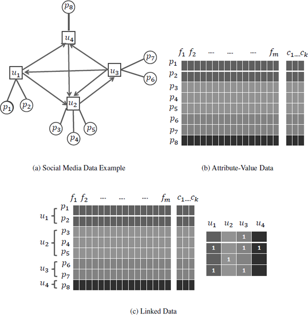
Most existing algorithms of feature selection for classification work with generic datasets and always assume that data is independent and identically distributed. With the development of social media, linked data is available where instances contradict the i.i.d. assumption.
Linked data has become ubiquitous in real-world applications such as tweets in Twitter1 (tweets linked through hyperlinks), social networks in Facebook2 (people connected by friendships), and biological networks (protein interaction networks). Linked data is patently not independent and identically distributed (i.i.d.), which is among the most enduring and deeply buried assumptions of traditional machine learning methods [31, 63]. Figure 2.10 shows a typical example of linked data in social media. Social media data is intrinsically linked via various types of relations such as user-post relations and user-user relations.
Many linked-data-related learning tasks are proposed, such as collective classification [47, 59], and relational clustering [44, 45], but the task of feature selection for linked data is rarely touched. Feature selection methods for linked data need to solve the following immediate challenges:
- How to exploit relations among data instances; and
- How to take advantage of these relations for feature selection.
Two attempts to handle linked data w.r.t. feature selection for classification are LinkedFS [62] and FSNet [16]. FSNet works with networked data and is supervised, while LinkedFS works with social media data with social context and is semi-supervised. In LinkedFS, various relations (co- Post, coFollowing, coFollowed, and Following) are extracted following social correlation theories. LinkedFS significantly improves the performance of feature selection by incorporating these relations into feature selection. There are many issues needing further investigation for linked data, such as handling noise, and incomplete and unlabeled linked social media data.
Acknowledgments
We thank Daria Bazzi for useful comments on the representation, and helpful discussions from Yun Li and Charu Aggarwal about the content of this book chapter. This work is, in part, supported by the National Science Foundation under Grant No. IIS-1217466.
Bibliography
[1] S. Alelyani, J. Tang, and H. Liu. Feature selection for clustering: A review. Data Clustering: Algorithms and Applications, Editors: Charu Aggarwal and Chandan Reddy, CRC Press, 2013.
[2] S. Alelyani, L. Wang, and H. Liu. The effect of the characteristics of the dataset on the selection stability. In Proceedings of the 23rd IEEE International Conference on Tools with Artificial Intelligence, 2011.
[3] F. R. Bach. Consistency of the group Lasso and multiple kernel learning. The Journal of Machine Learning Research, 9:1179–1225, 2008.
[4] H. D. Bondell and B. J. Reich. Simultaneous regression shrinkage, variable selection, and supervised clustering of predictors with oscar. Biometrics, 64(1):115–123, 2008.
[5] P. S. Bradley and O. L. Mangasarian. Feature selection via concave minimization and support vector machines. Proceedings ofthe Fifteenth International Conference on Machine Learning (ICML ’98), 82–90. Morgan Kaufmann, 1998.
[6] E. Candes and T. Tao. The Dantzig selector: Statistical estimation when p is much larger than n. The Annals of Statistics, 35(6):2313–2351, 2007.
[7] H. Y. Chuang, E. Lee, Y.T. Liu, D. Lee, and T. Ideker. Network-based classification of breast cancer metastasis. Molecular Systems Biology, 3(1), 2007.
[8] M. Dash and H. Liu. Feature selection for classification. Intelligent Data Analysis, 1(1–4):131–156, 1997.
[9] C. Domeniconi and D. Gunopulos. Local feature selection for classification. Computational Methods, page 211, 2008.
[10] R.O. Duda, P.E. Hart, andD.G. Stork. Pattern Classification. Wiley-Interscience, 2012.
[11] R.O. Duda, P.E. Hart, and D.G. Stork. Pattern Classification. New York: John Wiley & Sons, 2nd edition, 2001.
[12] J.G. Dy and C.E. Brodley. Feature subset selection and order identification for unsupervised learning. In In Proc. 17th International Conference on Machine Learning, pages 247–254. Morgan Kaufmann, 2000.
[13] J.G. Dy and C.E. Brodley. Feature selection for unsupervised learning. The Journal of Machine Learning Research, 5:845–889, 2004.
[14] J. Fan and R. Li. Variable selection via nonconcave penalized likelihood and its oracle properties. Journal of the American Statistical Association, 96(456):1348–1360, 2001.
[15] N. L. C. Talbot G. C. Cawley, and M. Girolami. Sparse multinomial logistic regression via Bayesian l1 regularisation. In Neural Information Processing Systems, 2006.
[16] Q. Gu, Z. Li, and J. Han. Towards feature selection in network. In International Conference on Information and Knowledge Management, 2011.
[17] Q. Gu, Z. Li, and J. Han. Generalized Fisher score for feature selection. arXiv preprint arXiv:1202.3725, 2012.
[18] I. Guyon and A. Elisseeff. An introduction to variable and feature selection. The Journal of Machine Learning Research, 3:1157–1182, 2003.
[19] I. Guyon, J. Weston, S. Barnhill, and V. Vapnik. Gene selection for cancer classification using support vector machines. Machine learning, 46(1–3):389–422, 2002.
[20] M.A. Hall and L.A. Smith. Feature selection for machine learning: Comparing a correlation-based filter approach to the wrapper. In Proceedings of the Twelfth International Florida Artificial Intelligence Research Society Conference, volume 235, page 239, 1999.
[21] T. Hastie, R. Tibshirani, and J. Friedman. The Elements of Statistical Learning. Springer, 2001.
[22] T. Hastie and R. Tibshirani. Discriminant adaptive nearest neighbor classification. IEEE Transactions on Pattern Analysis and Machine Intelligence, 18(6):607–616, 1996.
[23] J. Huang, J. L. Horowitz, and S. Ma. Asymptotic properties of bridge estimators in sparse high-dimensional regression models. The Annals of Statistics, 36(2):587–613, 2008.
[24] J. Huang, S. Ma, and C. Zhang. Adaptive Lasso for sparse high-dimensional regression models. Statistica Sinica, 18(4):1603, 2008.
[25] J. Huang, T. Zhang, and D. Metaxas. Learning with structured sparsity. In Proceedings of the 26th Annual International Conference on Machine Learning, pages 417–424. ACM, 2009.
[26] I. Inza, P. Larrañaga, R. Blanco, and A. J. Cerrolaza. Filter versus wrapper gene selection approaches in dna microarray domains. Artificial intelligence in Medicine, 31(2):91–103, 2004.
[27] L. Jacob, G. Obozinski, and J. Vert. Group Lasso with overlap and graph Lasso. In Proceedings of the 26th Annual International Conference on Machine Learning, pages 433–440. ACM, 2009.
[28] G. James, P. Radchenko, and J. Lv. Dasso: Connections between the Dantzig selector and Lasso. Journal of the Royal Statistical Society: Series B (Statistical Methodology), 71(1):127–142, 2009.
[29] R. Jenatton, J. Audibert, and F. Bach. Structured variable selection with sparsity-inducing norms. Journal of Machine Learning Research, 12:2777–2824,2011.
[30] R. Jenatton, J. Mairal, G. Obozinski, and F. Bach. Proximal methods for sparse hierarchical dictionary learning. Journal of Machine Learning Research, 12:2297–2334, 2011.
[31] D. Jensen and J. Neville. Linkage and autocorrelation cause feature selection bias in relational learning. In International Conference on Machine Learning, pages 259–266, 2002.
[32] S. Kim and E. Xing. Statistical estimation of correlated genome associations to a quantitative trait network. PLoS Genetics, 5(8):e1000587,2009.
[33] S. Kim and E. Xing. Tree-guided group Lasso for multi-task regression with structured spar-sity. In Proceedings of the 27th International Conference on Machine Learing, Haifa, Israel, 2010.
[34] K. Kira and L. Rendell. A practical approach to feature selection. In Proceedings ofthe Ninth International Workshop on Machine Learning, pages 249–256. Morgan Kaufmann Publishers Inc., 1992.
[35] K. Knight and W. Fu. Asymptotics for Lasso-type estimators. Annals of Statistics, 78(5):1356–1378, 2000.
[36] R. Kohavi and G.H. John. Wrappers for feature subset selection. Artificial Intelligence, 97(1–2):273–324, 1997.
[37] D. Koller and M. Sahami. Toward optimal feature selection. In Proceedings of the International Conference on Machine Learning, pages 284–292, 1996.
[38] H. Liu and H. Motoda. Feature selection for knowledge discovery and data mining, volume 454. Springer, 1998.
[39] H. Liu and H. Motoda. Computational Methods of Feature Selection. Chapman and Hall/CRC Press, 2007.
[40] H. Liu and L. Yu. Toward integrating feature selection algorithms for classification and clustering. IEEE Transactions on Knowledge and Data Engineering, 17(4):491, 2005.
[41] J. Liu, S. Ji, and J. Ye. Multi-task feature learning via efficient l 2, 1-norm minimization. In Proceedings of the Twenty-Fifth Conference on Uncertainty in Artificial Intelligence, pages 339–348. AUAI Press, 2009.
[42] J. Liu and J. Ye. Moreau-Yosida regularization for grouped tree structure learning. Advances in Neural Information Processing Systems, 187:195–207,2010.
[43] Z. Liu, F. Jiang, G. Tian, S. Wang, F. Sato, S. Meltzer, and M. Tan. Sparse logistic regression with lp penalty for biomarker identification. Statistical Applications in Genetics and Molecular Biology, 6(1), 2007.
[44] B. Long, Z.M. Zhang, X. Wu, and P.S. Yu. Spectral clustering for multi-type relational data. In Proceedings ofthe 23rd International Conference on Machine Learning, pages 585–592. ACM, 2006.
[45] B. Long, Z.M. Zhang, and P.S. Yu. A probabilistic framework for relational clustering. In Proceedings ofthe 13th ACM SIGKDD International Conference on Knowledge Discovery and Data Mining, pages 470–479. ACM, 2007.
[46] S. Ma and J. Huang. Penalized feature selection and classification in bioinformatics. Briefings in Bioinformatics, 9(5):392–403,2008.
[47] S.A. Macskassy and F. Provost. Classification in networked data: A toolkit and a univariate case study. The Journal of Machine Learning Research, 8:935–983,2007.
[48] M. Masaeli, J G Dy, and G. Fung. From transformation-based dimensionality reduction to feature selection. In Proceedings ofthe 27th International Conference on Machine Learning, pages 751–758, 2010.
[49] J. McAuley, J Ming, D. Stewart, and P. Hanna. Subband correlation and robust speech recognition. IEEE Transactions on Speech and Audio Processing, 13(5):956–964, 2005.
[50] L. Meier, S. De Geer, and P. Bühlmann. The group Lasso for logistic regression. Journal of the Royal Statistical Society: Series B (Statistical Methodology), 70(1):53–71, 2008.
[51] P. Mitra, C. A. Murthy, and S. Pal. Unsupervised feature selection using feature similarity. IEEE Transactions on Pattern Analysis andMachine Intelligence, 24:301–312, 2002.
[52] H. Peng, F. Long, and C. Ding. Feature selection based on mutual information: Criteria of max-dependency, max-relevance, and min-redundancy. IEEE Transactions on Pattern Analysis and Machine Intelligence, pages 1226–1238, 2005.
[53] S. Perkins and J. Theiler. Online feature selection using grafting. In Proceedings of the International Conference on Machine Learning, pages 592–599, 2003.
[54] J. R. Quinlan. C4.5: Programs for Machine Learning. Morgan Kaufmann, 1993.
[55] J. R. Quinlan. Induction of decision trees. Machine Learning, 1(1):81–106, 1986.
[56] M. Robnik Sikonja and I. Kononenko. Theoretical and empirical analysis of ReliefF and RReliefF. Machine Learning, 53(1–2):23–69, 2003.
[57] Y. Saeys, I. Inza, and P. Larrañaga. A review of feature selection techniques in bioinformatics. Bioinformatics, 23(19):2507–2517, 2007.
[58] T. Sandler, P. Talukdar, L. Ungar, and J. Blitzer. Regularized learning with networks of features. Neural Information Processing Systems, 2008.
[59] P. Sen, G. Namata, M. Bilgic, L. Getoor, B. Galligher, and T. Eliassi-Rad. Collective classification in network data. AI Magazine, 29(3):93,2008.
[60] M. R. Sikonja and I. Kononenko. Theoretical and empirical analysis of ReliefF and RReliefF. Machine Learning, 53:23–69, 2003.
[61] L. Song, A. Smola, A. Gretton, K. Borgwardt, and J. Bedo. Supervised feature selection via dependence estimation. In Proceedings of the 24th International Conference on Machine Learning, pages 823–830, 2007.
[62] J. Tang and H. Liu. Feature selection with linked data in social media. In SDM, pages 118–128, 2012.
[63] B. Taskar, P. Abbeel, M.F. Wong, and D. Koller. Label and link prediction in relational data. In Proceedings of the IJCAI Workshop on Learning Statistical Models from Relational Data. Citeseer, 2003.
[64] R. Tibshirani. Regression shrinkage and selection via the Lasso. Journal ofthe Royal Statistical Society. Series B (Methodological), pages 267–288, 1996.
[65] R. Tibshirani, M. Saunders, S. Rosset, J. Zhu, and K. Knight. Sparsity and smoothness via the fused Lasso. Journal ofthe Royal Statistical Society: Series B (Statistical Methodology), 67(1):91–108, 2005.
[66] R. Tibshirani and P. Wang. Spatial smoothing and hot spot detection for cgh data using the fused Lasso. Biostatistics, 9(1):18–29, 2008.
[67] J. Wang, P. Zhao, S. Hoi, and R. Jin. Online feature selection and its applications. IEEE Transactions on Knowledge and Data Engineering, pages 1–14, 2013.
[68] J. Weston, A. Elisseff, B. Schoelkopf, and M. Tipping. Use of the zero norm with linear models and kernel methods. Journal of Machine Learning Research, 3:1439–1461, 2003.
[69] D. Wettschereck, D. Aha, and T. Mohri. A review and empirical evaluation of feature weighting methods for a class of lazy learning algorithms. Artificial Intelligence Review, 11:273–314, 1997.
[70] X. Wu, K. Yu, H. Wang, and W. Ding. Online streaming feature selection. In Proceedings of the 27th International Conference on Machine Learning, pages 1159–1166, 2010.
[71] Z. Xu, R. Jin, J. Ye, M. Lyu, and I. King. Discriminative semi-supervised feature selection via manifold regularization. In IJCAI’09: Proceedings of the 21th International Joint Conference on Artificial Intelligence, 2009.
[72] S. Yang, L. Yuan, Y. Lai, X. Shen, P. Wonka, and J. Ye. Feature grouping and selection over an undirected graph. In Proceedings of the 18th ACM SIGKDD International Conference on Knowledge Discovery and Data Mining, pages 922–930. ACM, 2012.
[73] J. Ye and J. Liu. Sparse methods for biomedical data. ACM SIGKDD Explorations Newsletter, 14(1):4–15,2012.
[74] L. Yu and H. Liu. Feature selection for high-dimensional data: A fast correlation-based filter solution. In International Conference on Machine Learning, 20:856, 2003.
[75] M. Yuan and Y. Lin. Model selection and estimation in regression with grouped variables. Journal of the Royal Statistical Society: Series B (Statistical Methodology),68(1):49–67, 2006.
[76] P. Zhao and B. Yu. On model selection consistency of Lasso. Journal of Machine Learning Research, 7:2541–2563, 2006.
[77] Z. Zhao and H. Liu. Semi-supervised feature selection via spectral analysis. In Proceedings of SIAM International Conference on Data Mining, 2007.
[78] D. Zhou, J. Huang, and B. Scholkopf. Learning from labeled and unlabeled data on a directed graph. In International Conference on Machine Learning, pages 1036–1043. ACM, 2005.
[79] J. Zhou, J. Liu, V. Narayan, and J. Ye. Modeling disease progression via fused sparse group Lasso. In Proceedings of the 18th ACM SIGKDD International Conference on Knowledge Discovery and Data Mining, pages 1095–1103. ACM, 2012.
[80] H. Zou. The adaptive lasso and its oracle properties. Journal ofthe American Statistical Association, 101(476):1418–1429, 2006.
[81] H. Zou and T. Hastie. Regularization and variable selection via the elastic net. Journal of the Royal Statistical Society: Series B (Statistical Methodology), 67(2):301–320, 2005.