
Once a dataset has been filtered and shaped (as covered in the previous chapter), it probably still needs a good few modifications to make it ready for consumption. Many of these modifications are, at their heart, a series of fairly simple yet necessary techniques that you apply to make the data cleaner and more standardized. I have chosen to group these approaches under the heading data transformation.
Change the data type for a column—by telling Power Query that the column contains numbers, for example
Ensure that the first row is used as headers (if this is required)
Remove part of a column’s contents
Replace the values in a cell with other values
Transform the column contents—by making the text uppercase, for instance, or by removing decimals from numbers
Fill data down or up over empty cells to ensure that records are complete
Apply math or statistical (or even trigonometric) functions to columns of numbers
Convert date or time data into date elements such as days, months, quarters, years, hours, or minutes
Duplicating a column and possibly altering the format of the data in the copied column
Extracting part of the data in a column into a new column
Separating all the multiple data elements in a column so that each data element appears in a separate column
Merging columns into a new column
Adding custom columns that possibly contain calculations or extract part of a column’s data into a new column or even concatenate columns
Adding “index” columns that number the rows to ensure uniqueness or memorize a sort order
This chapter will take you on a tour of these kinds of essential data transformations. Once you have finished reading it, you should be confident that you can take a rough and ready data source as a starting point and convert it into a polished and coherent data table that is ready to become a pivotal part of your Excel analytics. Not only that, but you will have carried out really heavy lifting much faster and more easily than you could have done using enterprise-level tools or most of the Excel techniques that you know already.
The sample data that you will need to follow the exercises in this chapter is in the folder C:DataMashupWithExcelSamples.
Viewing a Full Record
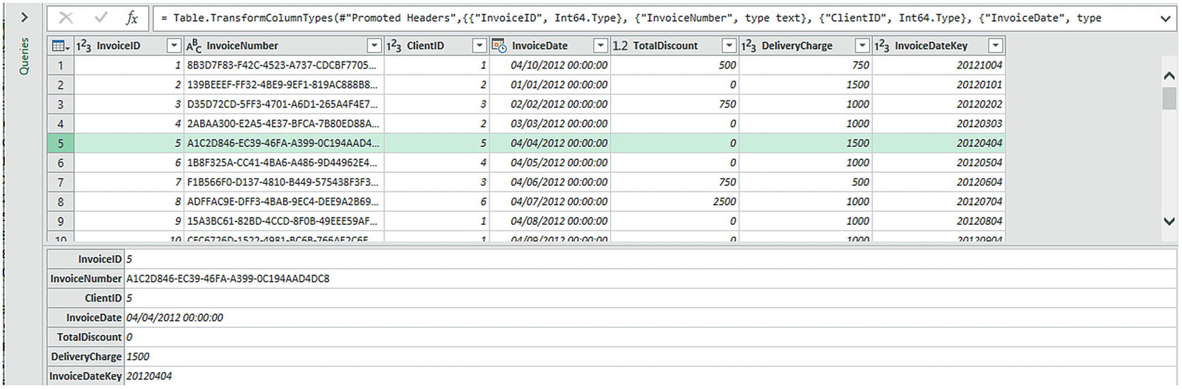
Before even starting to cleanse data, you probably need to take a good look at it. While the Power Query Editor is great for scrolling up and down columns to see how data compares for a single field, it is often less easy to appreciate the entire contents of a single record.
Viewing a full record
You can alter the relative height of the recordset and dataset windows simply by dragging the gray separator line between the upper and lower windows up or down.
Power Query Editor Context Menus
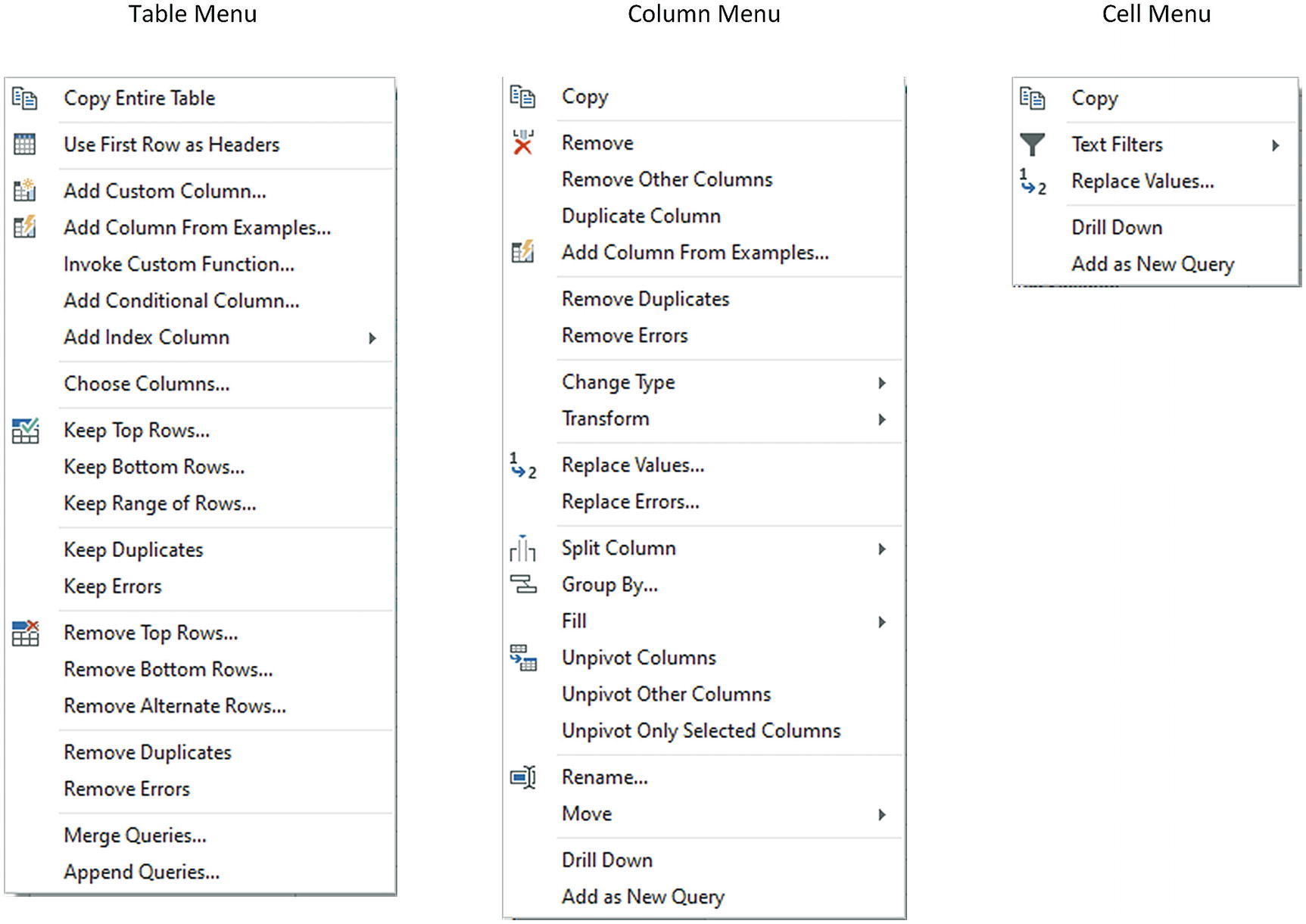
Table menu: This menu appears when you right-click the top corner of the grid containing the data (or click the small triangle at the top left of the data grid).
Column menu: This menu appears when you right-click a column title.
Cell menu: This menu appears when you right-click a data cell.
The Power Query Editor context menus
Because the options that are available in the context menus are explained throughout this, the previous, and the following chapters, I will not explain them all in detail here.
The cell context menu will reflect the data type of the cell in the filter option. So a numeric cell will have the option “Number filters.”
Using the First Row as Headers
You avoid leaving the columns named Column1, Column2, and so on. Leaving them named generically like this would make it needlessly difficult for a user (or even yourself) to understand the data.
You avoid having a text element (which should be the column title) in a column of figures, which can cause problems later on. This is because a whole column needs to have the same data type for another data type to be applied. Having a header text in the first row prevents this for numeric and date/time data types, for instance. This could be because the header is a text, whereas the remainder of the column contains numbers or dates.
- 1.
Click Use First Row as Headers in the Transform ribbon of the Power Query window.
After a few seconds, the first record disappears and the column titles become the elements that were in the first record. The Applied Steps list on the right now contains a Promoted Headers element, indicating which process has taken place. This step is highlighted.
Power Query is often able to apply this step automatically when the source is a database. It can often correctly guess when the source is a file. However, it cannot always guess accurately, so sometimes you have to intervene. You can see if Power Query has had to guess that the first row contained headers if it has added a Promoted Headers step to the Applied Steps list.
In the rare event that Power Query gets this operation wrong and presumes that a first row is column titles when it is not, you can reset the titles to be the first row by clicking the tiny triangle to the right of the Use First Row as Headers button. This displays a short menu where you can click the Use Headers as First Row option. The Applied Steps list on the right now contains a Demoted Headers element and the column titles are Column1, Column2, and so forth. You can subsequently rename the columns as you see fit.
Changing Data Type
A truly fundamental aspect of data modification is ensuring that the data is of the appropriate type; that is, if you have a column of numbers that are to be calculated at some point, then the column should be a numeric column. If it contains dates, then it should be set to one of the date or time data types. I realize that this can seem arduous and even superfluous; however, if you want to be sure that your data can be sliced and diced correctly further down the line, then setting the right data types at the outset is vital. An added bonus is that if you validate the data types early on in the process of loading data, you can see from the start if the data has any potential issues—dates that cannot be read as dates, for instance. This allows you to decide what to do with poor or unreliable data early in your work with a dataset.
The good news here is that for many data sources, Power Query applies an appropriate data type. Specifically, if you have loaded data from a database, then Power Query will recognize the source data type for each column and apply a suitable Power Query data type as the database has supplied the necessary information for Power Query to apply the correct data type. Unfortunately, things can get a little more painful with file sources, specifically CSV, text, and (occasionally) Excel files, as well as some XML files. In the case of these file types, Power Query often tries to guess the data type, but there are times when it does not succeed. If it has made a stab at deducing data types, then you see a Changed Type step in the Applied Steps list. Consequently, if you are obtaining your data from these sources, then you could well be obliged to apply data types to many of the columns manually.
In some cases, numbers are not meant to be interpreted as numerical data. For instance, a French postal code is five numbers, but it will never be calculated in any way. So it is good practice to let Power Query know this by changing the data type to text in cases when a numeric data type is inappropriate.
- 1.
Load the C:DataMashupWithExcelSamplesChapter07Example1.xlsx sample file.
- 2.
Display the Queries & Connections pane by clicking Queries & Connections in the Data ribbon (unless this pane is already visible).
- 3.
Double-click the BaseData query in the Queries & Connections pane to switch to the Query Editor.
- 4.
Click inside the column whose data type you wish to change. If you want to modify several columns, then Ctrl-click the requisite column titles. In this example, you could select the CostPrice and TotalDiscount columns.
- 5.
Click the Data Type button in the Transform ribbon. A popup menu of potential data types will appear.
- 6.
Select an appropriate data type. If you have selected the CostPrice and TotalDiscount columns, then Whole Number is the type to choose.
Data Types in Power Query
Data Type | Description |
|---|---|
Decimal Number | Converts the data to a decimal number |
Fixed Decimal Number | Converts the data to a decimal number with a fixed number of decimals |
Whole Number | Converts the data to a whole (integer) number |
Date/Time | Converts to a date and time data type |
Date | Converts to a date data type |
Time | Converts to a time data type |
Duration | Sets the data as being a duration. These are used for date and time calculations |
Text | Sets to a text data type |
True/False | Sets the data type to Boolean (True or False) |
Binary | Defines the data as binary, and consequently, it is not directly visible |
The Data Type button is also available in the Home ribbon. Equally, you can right-click a column header and select Change Type to select a different data type.
Inevitably, there will be times when you try to apply a data type that simply cannot be used with a certain column of data. Converting a text column (such as Make in this sample data table) into dates will simply not work. If you do this, then Power Query will replace the column contents with Error. This is not definitive or dangerous, and all you have to do to return the data to its previous state is to delete the Changed Type step in the Applied Steps list using the technique described in the previous chapter.
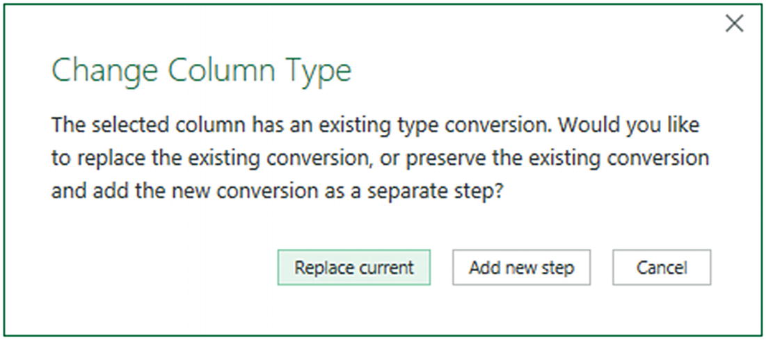
The Change Column Type alert
Let Power Query update the existing conversion step with the data type that you just selected.
Add a new conversion step.
Your choice will depend on exactly what type of transformation you are applying to the underlying dataset.
You can concentrate on getting data types right, and if you are working methodically, you are less likely to forget to set a data type.
Applying data types for many columns (even if you are doing this in several operations, to single or multiple columns) will only add a single step to the Applied Steps list.
Don’t look for any data formatting options in Power Query; there aren’t any. This is deliberate since this tool is designed to structure, load, and cleanse data, but not to present it. You carry out the formatting in the Excel as you are used to doing.
Detecting Data Types
- 1.
In the Transform ribbon, click the Detect Data Type button.
- 2.
Changed Type will appear in the Applied Steps list. Most of the columns will have the correct data type applied.
This technique does not always give perfect results, and there will be times when you want to override the choice of data type that Power Query has applied. Yet it is nonetheless a welcome addition to the data preparation toolset that can save you considerable time when preparing a dataset.
Data Type Indicators
Data Type Icons in Power Query Editor
Data Type Icon | Description |
|---|---|
| Any data type from among the possible data types |
| Whole Number |
| Decimal Number |
| Fixed Decimal Number |
| Percentage |
| Text |
| True/False |
| Date/Time |
| Date |
| Time |
| Date/Time/Timezone |
| Duration |
| Binary |
Switching Data Types
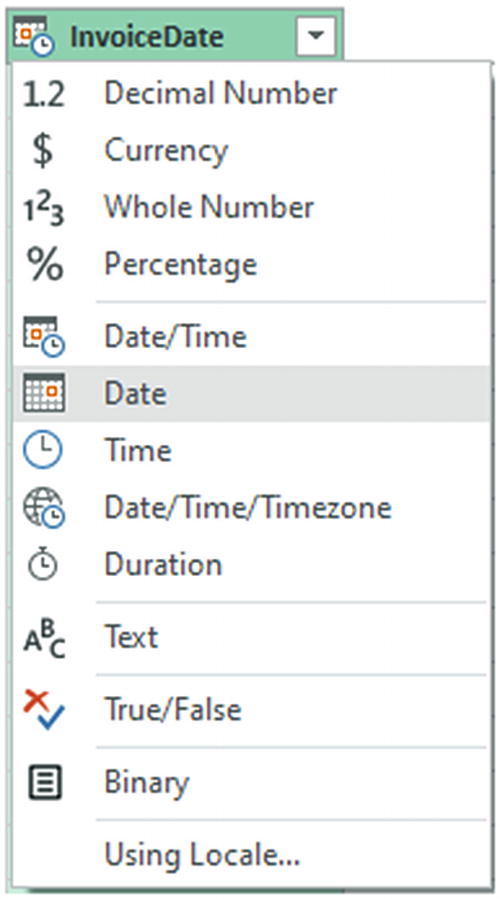
The data type context menu
Data Type Using Locale
- 1.
Open the Query Editor (from inside the source file C:DataMashupWithExcelSamplesChapter07Example1.pbix).
- 2.
Click the data type icon to the left of the column title.
- 3.
Select Using Locale from the popup menu. The Change Type with Locale dialog will appear.
- 4.
Choose the new data type to apply from the list of available data types.
- 5.
Select the required locale from the list of worldwide locales. The dialog will look like Figure 7-5.
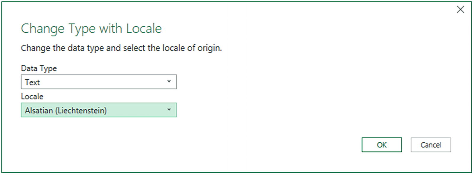
The Change Type with Locale dialog
- 6.
Click OK.
The data type will be converted to the selected locale. The Applied Steps list will contain a step entitled Changed Type with Locale.
Replacing Values
- 1.
Click the title of the column that contains the data that you want to replace. The column will become selected. In this example, I used the Model column.
- 2.
In the Home ribbon, click the Replace Values button. The Replace Values dialog will appear.
- 3.
In the Value To Find box, enter the text or number that you want to replace. I used Ghost in this example.
- 4.
In the Replace With box, enter the text or number that you want to replace. I used Fantôme in this example, as shown in Figure 7-6.
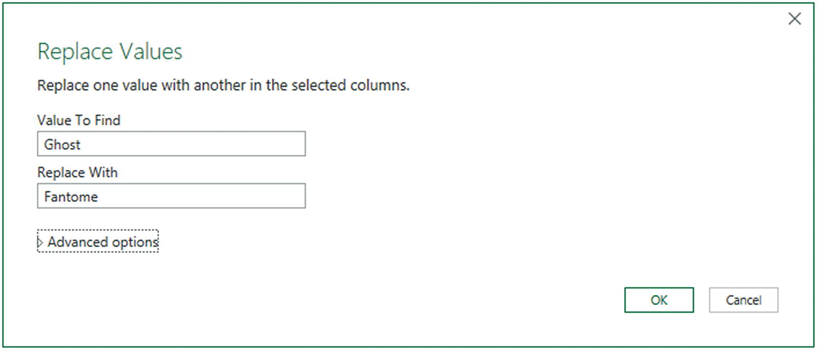
The Replace Values dialog
- 5.
Click OK. The data is replaced in the entire column. Replaced Values is added to the Applied Steps list.
The Replace Values process searches for every occurrence of the text that you are looking for in each record of the selected columns. It does not look for the entire contents of the cell unless you specifically request this by checking the Match entire cell contents check box in the Advanced options.
If you click a cell containing the contents that you want to replace (rather than the column title, as we just did), before starting the process, Power Query automatically places the cell contents in the Replace Values dialog as the value to find.
You can only replace text in columns that contain text elements. This does not work with columns that are set as a numeric or date data type. Indeed, you will see a yellow alert triangle in the Replace Values dialog if you enter values that do not match the data type of the selected column(s).
- If you really have to replace parts of a date or figures in a numeric column with other dates or numbers, then you can
Convert the column to a text data type
Carry out the replace operation
Convert the column back to the original data type
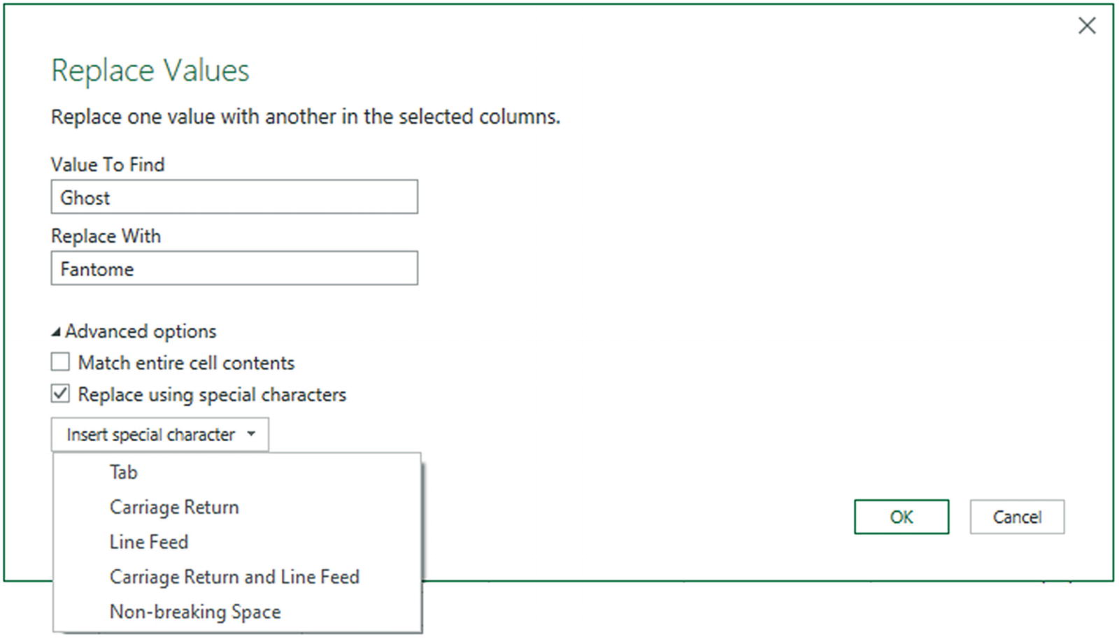
Advanced replace options
Advanced Replace Options
Option | Description |
|---|---|
Match entire cell contents | Only replaces the search value if it makes up the entire contents of the column for a row |
Replace using special characters | Replaces the search value with a nonprinting character |
Tab | Replaces the search value with a tab character |
Carriage Return | Replaces the search value with a carriage return character |
Line Feed | Replaces the search value with a line feed character |
Carriage Return and Line Feed | Replaces the search value with a carriage return and line feed |
Replacing words that are subsets of other words is dangerous. When replacing any data, make sure that you don’t damage elements other than the one you intend to change.
As a final and purely spurious comment, I must add that I would never suggest rebranding a Rolls Royce, as it would be close to automotive sacrilege.
Transforming Column Contents
Setting the capitalization of text columns
Rounding numeric data or applying math functions
Extracting date elements such as the year, month, or day (among others) from a date column
Power Query is very strict about applying transformations to appropriate types of data. This is because transforms are totally dependent on the data type of the selected column. This is yet another confirmation that applying the requisite data type is an operation that should be carried out early in any data transformation process—and certainly before transforming the column contents. Remember, you will only be able to select a numeric transformation if the column is a numeric data type, and you will only be able to select a date transformation if the column is a date data type. Equally, the text-based transformations can only be applied to columns that are of the text data type.
Text Transformation
- 1.
Still using the Query Editor opened from the file Chapter07Example1.xlsx, click anywhere in the column whose contents you wish to transform (Make, in this example).
- 2.
In the Transform ribbon, click the Format button. A popup menu will appear.
- 3.
Select UPPERCASE, as shown in Figure 7-8.
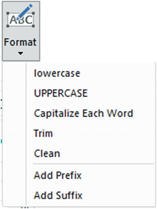
The Format menu
The contents of the entire column will be converted to uppercase. Uppercased Text will be added to the Applied Steps list.
Text Transformations
Transformation | Description | Applied Steps Definition |
|---|---|---|
Lowercase | Converts all the text to lowercase | Lowercased Text |
Uppercase | Converts all the text to uppercase | Uppercased Text |
Capitalize Each Word | Converts the first letter of each word to a capital | Capitalized Each Word |
Trim | Removes all spaces before and after the text | Trimmed Text |
Clean | Removes any nonprintable characters | Cleaned Text |
Add Prefix | Adds text at the start of the column contents | Added Prefix |
Add Suffix | Adds text at the end of the column contents | Added Suffix |
I realize that Power Query calls text transformations formatting. Nonetheless, these options are part of the overall data transformation options.
Adding a Prefix or a Suffix
- 1.
Click inside the column where you want to add a prefix.
- 2.
In the Transform ribbon, select Format ➤ Add Prefix. The Prefix dialog will be displayed, as you can see in Figure 7-9.
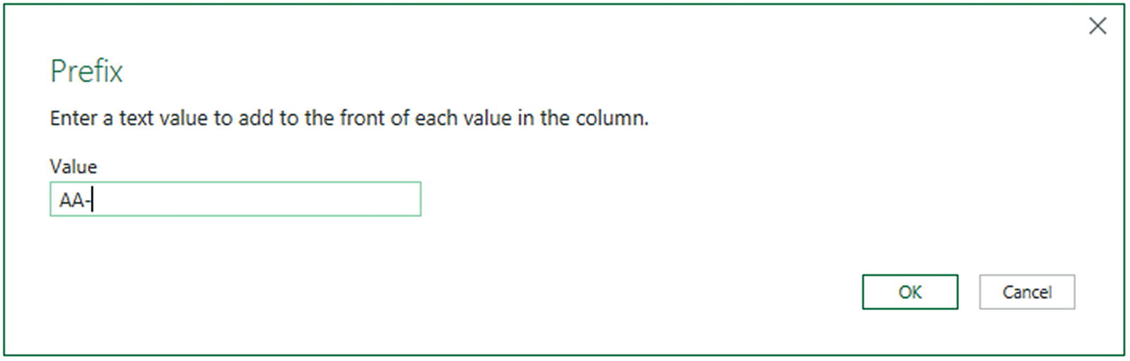
Adding a prefix to a text
- 3.
Enter the prefix to add in the Value field.
- 4.
Click OK.
The prefix that you designated will be placed at the start of every record in the dataset for the selected field.
If you add a prefix or a suffix to a numeric or date/time column, then the column data type will automatically be converted to text.
Removing Leading and Trailing Spaces
Data duplication, because a value with a trailing space is not considered identical to the same text without the spaces that follow
Sort issues, because a leading space causes an element to appear at the top of a sorted list
Grouping errors, because elements with spaces are not part of the same group as elements without spaces
- 1.
Click anywhere in the column whose contents you wish to transform (Make, in this case).
- 2.
In the Transform ribbon, click the Format button. A popup menu will appear.
- 3.
Select Trim from the menu.
All superfluous leading and trailing spaces will be removed from the data in the column. This can help when sorting, grouping, and deduplicating records.
Removing Nonprinting Characters
Some source data can contain somewhat insidious elements called nonprinting characters. These can, even if they are nearly always invisible to humans, cause problems in certain circumstances.
- 1.
Click inside the column (or select the columns) that you know to contain (or that you suspect contain) nonprinting characters.
- 2.
Click Format➤ Clean.
Power Query will add Cleaned Text to the list of Applied Steps.
Number Transformations
- 1.
Open the Query Editor for the Excel file Chapter07Sample1.xlsx (unless already open, of course).
- 2.
Click anywhere in the column whose contents you wish to transform (TotalDiscount, in this case).
- 3.
In the Transform ribbon, click the Rounding button. A popup menu will appear, showing all the available options. You can see this in Figure 7-10.
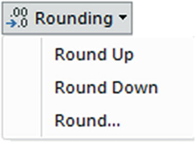
Rounding options
- 4.
Select Round Up.
The values in the entire column will be rounded up to the nearest whole number. Rounded Up will be added to the Applied Steps list.
Number Transformations
Transformation | Description | Applied Steps Definition |
|---|---|---|
Rounding ➤ Round Up | Rounds each number to the specified number of decimal places | Rounded Up |
Rounding ➤ Round Down | Rounds each number down | Rounded Down |
Round… | Rounds each number to the number of decimals that you specify. If you specify a negative number, you round to a given decimal | Rounded Off |
Scientific ➤ Absolute Value | Makes the number absolute (positive) | Absolute Value |
Scientific ➤ Power ➤ Square | Returns the square of the number in each cell | Calculated Square |
Scientific ➤ Power ➤ Cube | Returns the cube of the number in each cell | Calculated Cube Value |
Scientific ➤ Power ➤ Power | Raises each number to the power that you specify | Calculated Power |
Scientific ➤ Square Root | Returns the square root of the number in each cell | Calculated Square Root |
Scientific ➤ Exponent | Returns the exponent of the number in each cell | Calculated Exponent |
Scientific ➤ Logarithm ➤ Base 10 | Returns the base 10 logarithm of the number in each cell | Calculated Base 10 Logarithm |
Scientific ➤ Logarithm ➤ Natural | Returns the natural logarithm of the number in each cell | Calculated Natural Logarithm |
Scientific ➤ Factorial | Gives the factorial of numbers in the column | Calculated Factorial |
Trigonometry ➤ Sine | Gives the sine of the numbers in the column | Calculated Sine |
Trigonometry ➤ Cosine | Gives the cosine of the numbers in the column | Calculated Cosine |
Trigonometry ➤ Tangent | Gives the tangent of the numbers in the column | Calculated Tangent |
Trigonometry ➤ ArcSine | Gives the arcsine of the numbers in the column | Calculated ArcSine |
Trigonometry ➤ ArcCosine | Gives the arccosine of the numbers in the column | Calculated ArcCosine |
Trigonometry ➤ ArcTangent | Gives the arctangent of the numbers in the column | Calculated ArcTangent |
Power Query will not even let you try to apply numeric transformation to texts or dates. The relevant buttons remain grayed out if you click inside a column of letters or dates.
Calculating Numbers
- 1.
Click inside any column of numbers. In this example, I used the column SalePrice.
- 2.
Click the Standard button in the Transform ribbon. The menu will appear as you can see in Figure 7-11.
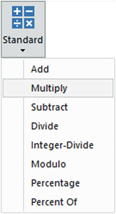
Applying a calculation to a column
- 3.
Click Multiply. The Multiply dialog will appear.
- 4.
Enter 1.1 in the Value box. The dialog will look like the one shown in Figure 7-12.
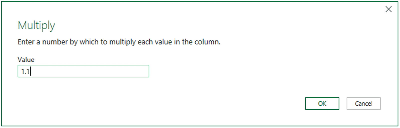
Applying a calculation to a column
- 5.
Click OK.
Applying Basic Calculations
Transformation | Description | Applied Steps Definition |
|---|---|---|
Add | Adds a selected value to the numbers in a column | Added to Column |
Multiply | Multiplies the numbers in a column by a selected value | Multiplied Column |
Subtract | Subtracts a selected value from the numbers in a column | Subtracted from Column |
Divide | Divides the numbers in a column by a selected value | Divided Column |
Integer-Divide | Divides the numbers in a column by a selected value and removes any remainder | Integer-Divided Column |
Modulo | Divides the numbers in a column by a selected value and leaves only the remainder | Calculated Modulo |
Percentage | Applies the selected percentage to the column | Calculated Percentage |
Percent Of | Expresses the value in the column as a percent of the value that you enter | Calculated Percent Of |
You can also carry out many types of calculations in Excel and avoid carrying out calculations in the Query Editor. Indeed, many Excel purists seem to prefer that anything resembling a calculation should take place inside the spreadsheet rather than at the Query stage. I will let you decide which approach you prefer.
Finally, it is important to remember that you are altering the data when you carry out this kind of operation. In the real world, you might be safer duplicating a column before profoundly altering the data it contains. This allows you to keep the initial data available, albeit at the cost of increasing both the load time and the size of the resulting Excel file.
Date Transformations
- 1.
Click inside the InvoiceDate column.
- 2.
In the Transform ribbon, click the Date button. The menu will appear.
- 3.
Click Year. The submenu will appear.
- 4.
Select Year. The year part of the date will replace all the dates in the InvoiceDate column.
Date Transformations
Transformation | Description | Applied Steps Definition |
|---|---|---|
Age | Calculates the date and time difference (in days and hours) between the original date and the current local time | Calculated Age |
Date Only | Converts the data to a date without the time element | Calculated Date |
Year ➤ Year | Extracts the year from the date | Calculated Year |
Year ➤ Start of Year | Returns the first day of the year for the date | Calculated Start of Year |
Year ➤ End of Year | Returns the last day of the year for the date | Calculated End of Year |
Month ➤ Month | Extracts the number of the month from the date | Calculated Month |
Month ➤ Start of Month | Returns the first day of the month for the date | Calculated Start of Month |
Month ➤ End of Month | Returns the last day of the month for the date | Calculated End of Month |
Month ➤ Days in Month | Returns the number of days in the month for the date | Calculated Days in Month |
Month ➤ Name of Month | Returns the name of the month for the date | Calculated Name of Month |
Day ➤ Day | Extracts the day from the date | Calculated Day |
Day ➤ Day of Week | Returns the weekday as a number (Monday is 1, Tuesday is 2, etc.) | Calculated Day of Week |
Day ➤ Day of Year | Calculates the number of days since the start of the year for the date | Calculated Day of Year |
Day ➤ Start of Day | Transforms the value to the start of the day for a date and time | Calculated Start of Day |
Day ➤ End of Day | Transforms the value to the end of the day for a date and time | Calculated End of Day |
Day ➤ Name of Day | Returns the weekday as a day of week | Calculated Name of Day |
Quarter ➤ Quarter | Returns the calendar quarter of the year for the date | Calculated Quarter |
Quarter ➤ Start of Quarter | Returns the first date of the calendar quarter of the year for the date | Calculated Start of Quarter |
Quarter ➤ End of Quarter | Returns the last date of the calendar quarter of the year for the date | Calculated End of Quarter |
Week ➤ Week of Year | Calculates the number of weeks since the start of the year for the date | Calculated Week of Year |
Week ➤ Week of Month | Calculates the number of weeks since the start of the month for the date | Calculated Week of Month |
Week ➤ Start of Week | Returns the date for the first day of the week (Monday) for the date | Calculated Start of Week |
Week ➤ End of Week | Returns the date for the last day of the week (Sunday) for the date | Calculated End of Week |
Time Transformations
- 1.
Click inside the InvoiceDate column.
- 2.
In the Transform ribbon, click the Time button. The menu will appear.
- 3.
Click Hour. The hour part of the time will replace all the values in the InvoiceDate column.
Time transformations can only be applied to columns of the date/time or time data types.
Time Transformations
Transformation | Description | Applied Steps Definition |
|---|---|---|
Time Only | Isolates the time part of a date and time | Extracted Time |
Local Time | Converts the date/time to local time from date/time and timezone values | Extracted Local Time |
Parse | Extracts the date and/or date/time elements from a text | Parsed DateTime |
Hour ➤ Hour | Isolates the hour from a date/time or date value | Extracted Hour |
Hour ➤ Start of Hour | Returns the start of the hour from a date/time or time value | Calculated Start of Hour |
Hour ➤ End of Hour | Returns the end of the hour from a date/time or time value | Calculated End of Hour |
Minute | Isolates the minute from a date/time or time value | Extracted Minute |
Second | Isolates the second from a date/time or time value | Extracted Second |
Earliest | Returns the earliest time from a date/time or time value | Calculated Earliest |
Latest | Returns the latest time from a date/time or time value | Calculated Latest |
In the real world, you could well want to leave a source column intact and apply number or date transformations to a copy of the column. To do this, simply apply the same transformation technique, only use the buttons in the Add Column ribbon instead of those in the Transform ribbon.
Duration
If you have values in a column that can be interpreted as a duration (in days, hours, minutes, and seconds), then Power Query can extract the component parts of the duration as a data transformation. For this to work, however, the column must be set to the duration data type. This means that the contents of the column have to be interpreted as a duration by Power Query. Any values that are incompatible with this data type will be set to error values.
Days
Hours
Minutes
Seconds
More specifically, a duration must be expressed in the form days.hours:minutes:seconds. So, for instance, a duration could be 11.23:5:45. This represents 11 days, 23 hours, 5 minutes, and 45 seconds.
The figure for days is followed by a period—the other separators are colons.
You cannot have the duration in hours greater than 23.
You cannot have the duration in minutes or seconds greater than 60.
- 1.
Open a new, blank Excel file.
- 2.
Click Data ➤ Get Data ➤ From File ➤ From Workbook and select the file C:DataMashupWithExcelSamplesDurations.xlsx.
- 3.
Click the worksheet Sheet1 and then click Transform Data to open the Query Editor. You will note that Power Query automatically adds a step that changes the data type of the DurationOnForecourt column to duration as it recognizes the data format.
- 4.
Click inside the column DurationOnForecourt.
- 5.
In the Transform ribbon, click the Duration button. The menu will appear.
- 6.
Click Hours. The hour part of the time will replace all the values in the InvoiceDate column.
Duration Transformations
Transformation | Description | Applied Steps Definition |
|---|---|---|
Days | Isolates the day element from a duration value | Extracted Days |
Hours | Isolates the hour element from a duration value | Extracted Hours |
Minutes | Isolates the minutes element from a duration value | Extracted Minutes |
Seconds | Isolates the seconds element from a duration value | Extracted Seconds |
Total Days | Displays the duration value as the number of days and a fraction representing hours, minutes, and seconds | Calculated Total Days |
Total Hours | Displays the duration value as the number of hours and a fraction representing minutes and seconds | Calculated Total Hours |
Total Minutes | Displays the duration value as the number of minutes and a fraction representing seconds | Calculated Total Minutes |
Total Seconds | Displays the duration value as the number of seconds and a fraction representing milliseconds | Calculated Total Seconds |
Multiply | Multiplies the duration (and all its component parts) by a value that you enter | Multiplied Column |
Divide | Divides the duration (and all its component parts) by a value that you enter | Divided Column |
Statistics ➤ Sum | Returns the total for all the duration elements in the column | Calculated Sum |
Statistics ➤ Minimum | Returns the minimum value of all the duration elements in the column | Calculated Minimum |
Statistics ➤ Maximum | Returns the maximum value of all the duration elements in the column | Calculated Maximum |
Statistics ➤ Median | Returns the median value for all the duration elements in the column | Calculated Median |
Statistics ➤ Average | Returns the average for all the duration elements in the column | Calculated Average |
If you multiply or divide a duration, Power Query displays a dialog so that you can enter the value to multiply or divide the duration by.
Filling Down Empty Cells
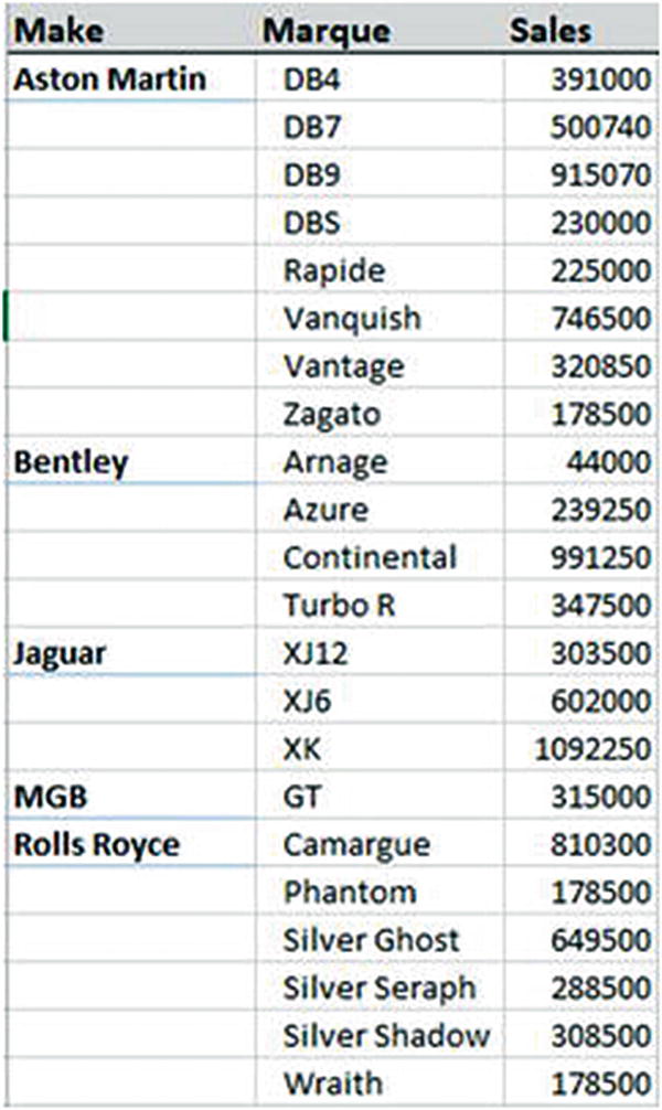
A matrix data table in Excel
- 1.
Open a new Excel file.
- 2.
In the Data ribbon, click Get Data ➤ From File ➤ From Workbook.
- 3.
In the Get Data dialog, select Excel. Then click Connect and navigate to C:DataMashupWithExcelSamplesCarMakeAndModelMatrix.xlsx.
- 4.
Click Import, select Sheet1, and click Transform Data. This will open the Power Query Editor.
- 5.
Select the column that contains the empty cells.
- 6.
In the Transform ribbon, click Fill. The menu will appear.
- 7.
Select Down. The blank cells will be replaced by the value in the first non-empty cell above. Filled Down will be added to the Applied Steps list.
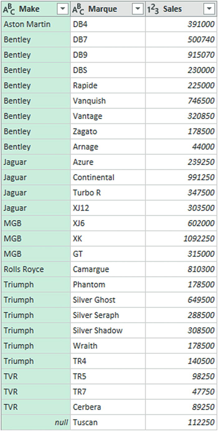
A data table with empty cells replaced by the correct data
This technique is built to handle a fairly specific problem and only really works if the imported data is grouped by the column containing the missing elements.
Although rare, you can also use this technique to fill empty cells with the value from below. If you need to do this, just select Fill ➤ Up from the Transform ribbon. In either case, you need to be aware that the technique is applied to the entire column.
Extracting Part of a Column’s Contents
- 1.
Load the C:DataMashupWithExcelSamplesChapter07Example1.xlsx sample file.
- 2.
Display the Queries & Connections pane by clicking Queries & Connections in the Data ribbon.
- 3.
Double-click the BaseData query to switch to the Query Editor.
- 4.
Click inside the InvoiceNumber column. As you can see, the invoice number is composed of multiple elements, each separated by a hyphen.
- 5.
In the Transform ribbon, click Extract ➤ Text Before Delimiter. The Text Before Delimiter dialog will be displayed.
- 6.
Enter a hyphen (or a minus sign) in the Delimiter field. The dialog will look like Figure 7-15.
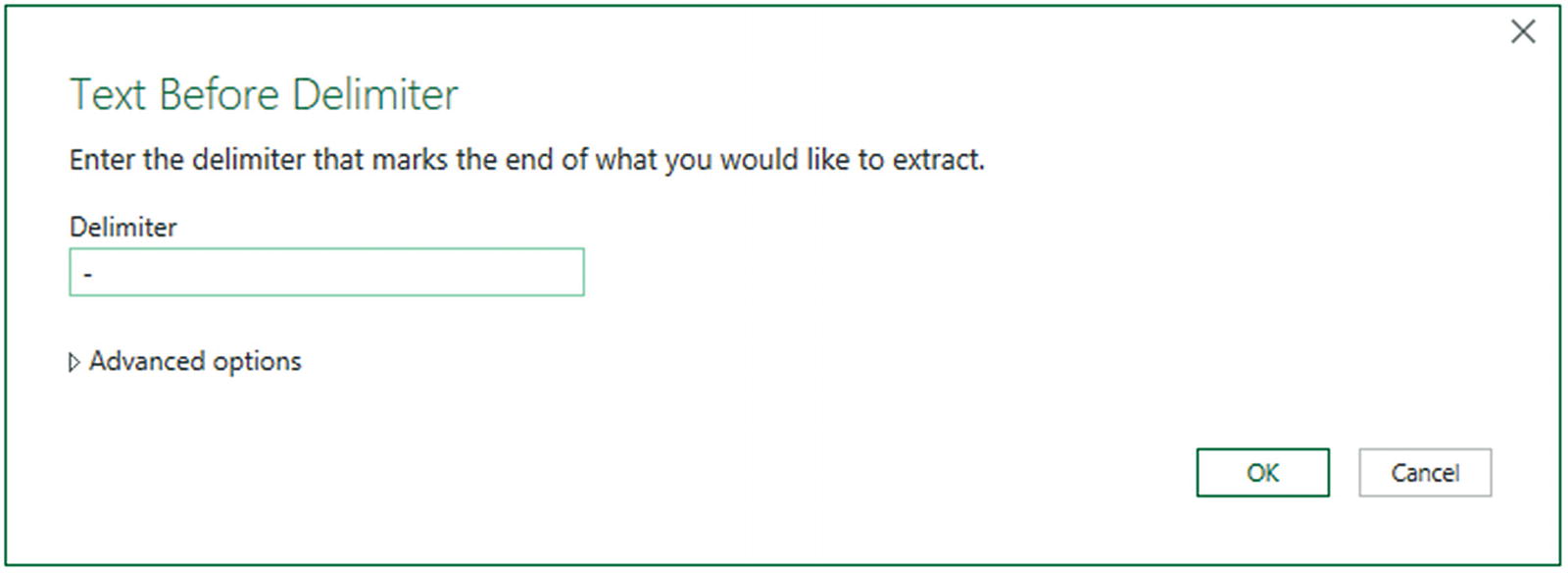
The Text Before Delimiter dialog
- 7.
Click OK. The contents of the field will be replaced by the characters before the hyphen. A step named Extracted Text Before Delimiter will be added to the Applied Steps list.
Extract Transformations
Transformation | Description | Applied Steps Definition |
|---|---|---|
Length | Displays the length in characters of the contents of the field | Extracted Length |
First Characters | Displays a specified number of characters from the left of the field | Extracted First Characters |
Last Characters | Displays a specified number of characters from the right of the field | Extracted Last Characters |
Range | Displays a specified number of characters between a specified start and end position (in characters, from the left of the field) | Extracted Range |
Text Before Delimiter | Displays all the text occurring before a specified character | Extracted Text Before Delimiter |
Text After Delimiter | Displays all the text occurring after a specified character | Extracted Text After Delimiter |
Text Between Delimiters | Displays all the text occurring between two specified characters | Extracted Text Between Delimiters |
Advanced Extract Options
Three of the Extract options (Text Before Delimiter, Text After Delimiter, and Text Between Delimiters) let you apply some advanced options that allow you to push the envelope even further when extracting data from a column. These techniques are explained in the following two sections.
Text Before and After Delimiter
If you are extracting data from the middle of a column and you are using a delimiter to isolate the text you want to keep, then you have a couple of additional options available.
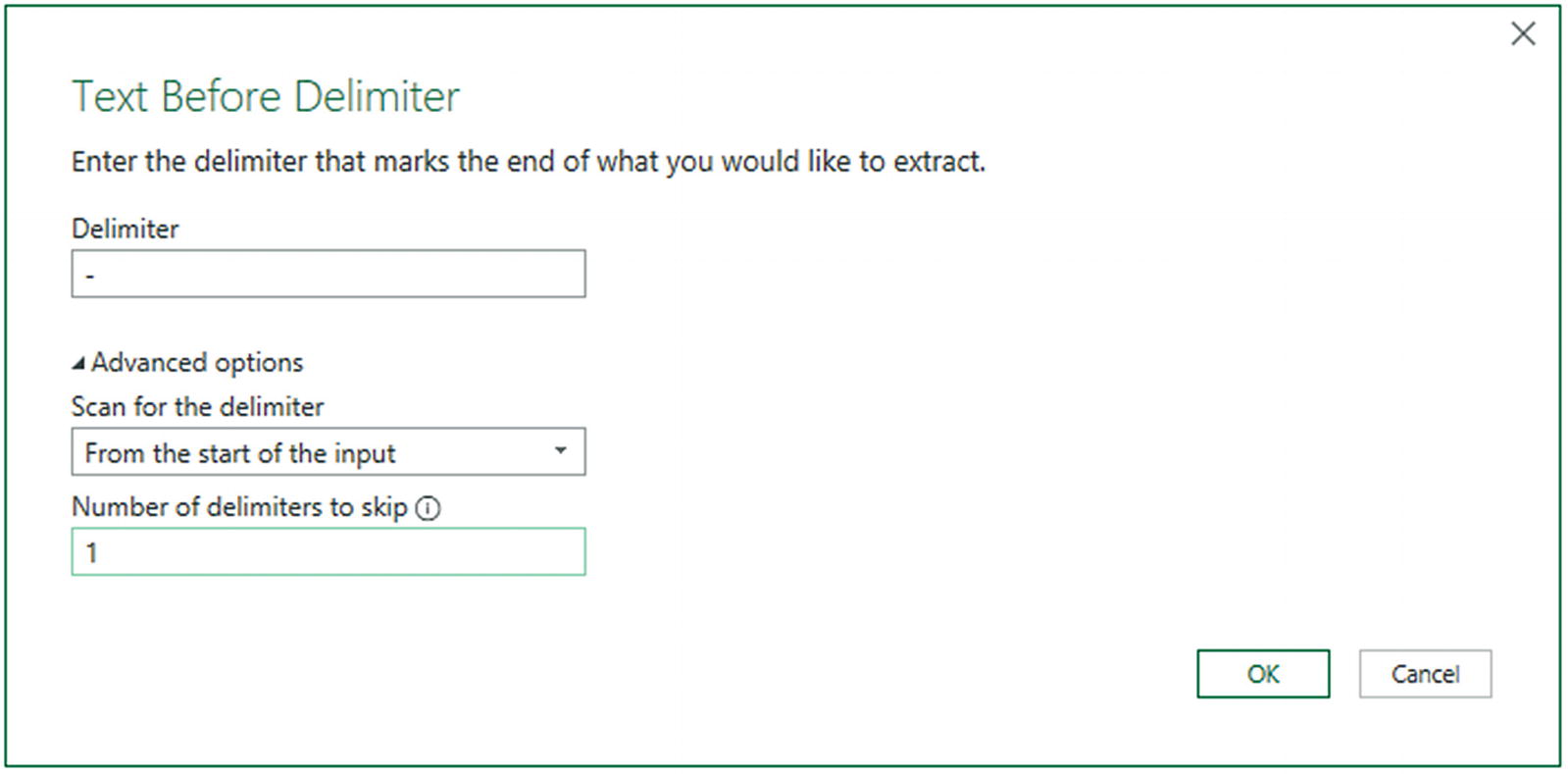
The Advanced options of the Text Before and Text After Delimiter dialogs
Scan for the delimiter: This option lets you choose between working forward from the start of the contents of the column and working backward from the end of the contents of the column to locate the delimiter you are searching for.
Number of delimiters to skip: Here you can specify that it is the nth occurrence of a delimiter that interests you.
Text Between Delimiters
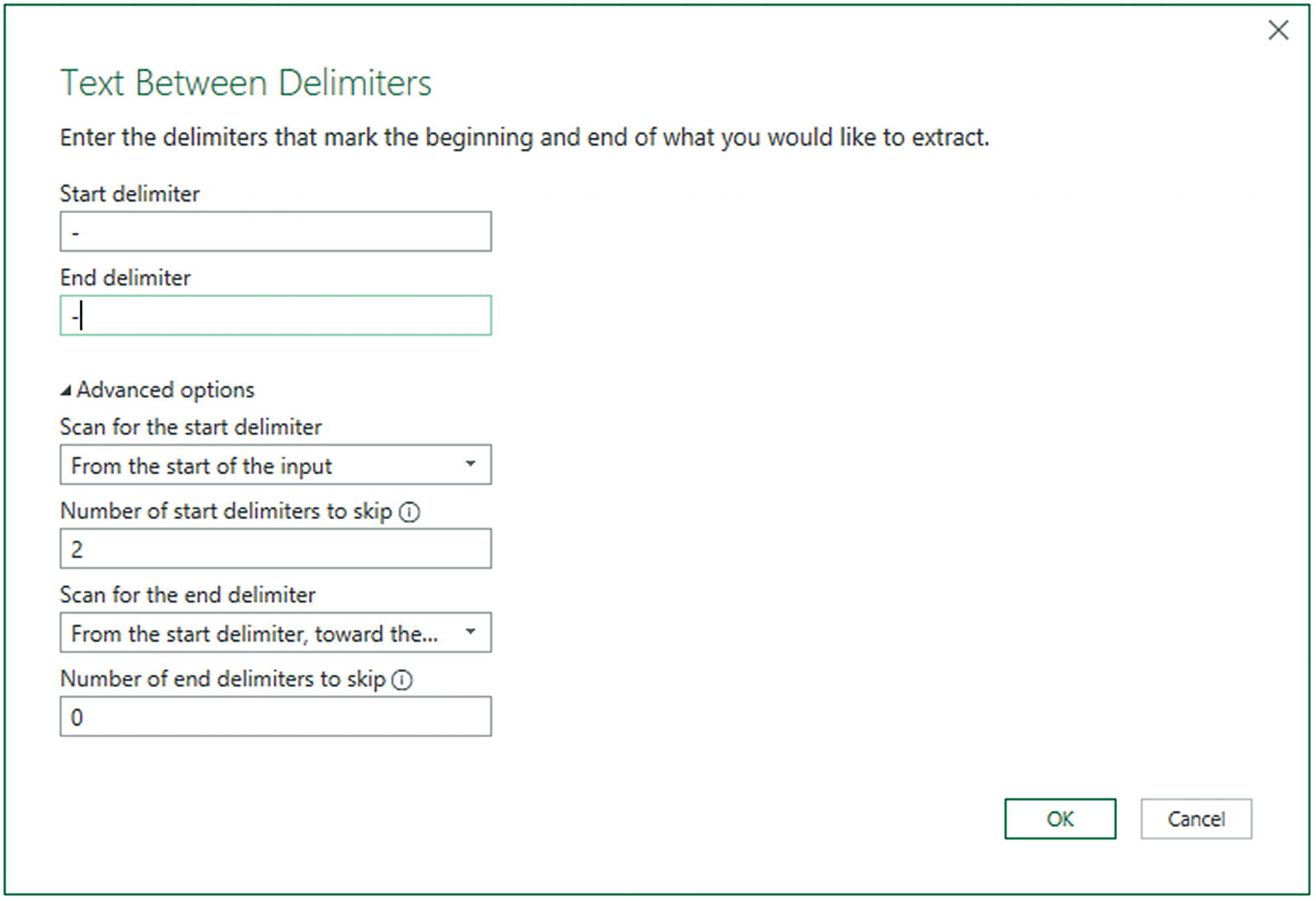
The Advanced options of the Text Between Delimiters dialog
The Extract button can be found in both the Transform and New Column ribbons. If you carry out this operation from the Transform ribbon, then the contents of the existing column will be replaced. If you use the button in the Add Column ribbon, then a new column containing the extracted text will be added at the right of any existing columns.
Duplicating Columns
- 1.
Load the C:DataMashupWithExcelSamplesChapter07 Example1.xlsx sample file.
- 2.
Switch to the Data ribbon and click Queries & Connections to display the Queries & Connections pane (unless it is already visible).
- 3.
Double-click the BaseData query to switch to the Query Editor.
- 4.
Click inside (or on the title of) the column that you want to duplicate. I will use the Make column in this example.
- 5.
In the Add Column ribbon, click the Duplicate Column button. After a few seconds, a copy of the column is created at the right of the existing table. Duplicated Column will appear in the Applied Steps list.
- 6.
Scroll to the right of the table and rename the existing column; it is currently named Make-Copy.
The duplicate column is named Original Column Name-Copy. I find that it helps to rename copies of columns sooner rather than later in a data mashup process.
Splitting Columns
A column contains a list of elements, separated by a specific character (known as a delimiter).
A column contains a list of elements, but the elements can be divided at specific places in the column.
A column contains a concatenated text that needs to be split into its composite elements (a bank account number or a Social Security number is an example of this).
The following short sections explain how to handle such eventualities.
Splitting Column by a Delimiter
Here is another requirement that you may encounter occasionally. The data that has been imported has a column that needs to be further split into multiple columns, and you want this to happen automatically. Imagine a text file where columns are separated by semicolons, and these subdivisions each contain a column that holds a comma-separated list of elements. Once you have imported the file, you then need to further separate the contents of this column that uses a different delimiter.
- 1.
Open a new Excel file.
- 2.
In the Data ribbon, click Get Data ➤ From File ➤ From Workbook.
- 3.
Select the C:DataMashupWithExcelSamplesDataToParse.xlsx sample file in the Query Editor.
- 4.
Click the ClientList workbook.
- 5.
Click Transform Data to open the Query Editor.
- 6.
In the Transform ribbon, click Use First Row as Headers.
- 7.
Click inside the ClientList column. You can see that this column contains several data elements, each separated by a semicolon.
- 8.
In the Transform ribbon, click Split Column ➤ By Delimiter. The Split Column by Delimiter dialog appears.
- 9.
Select Semicolon from the list of available options in the “Select or enter delimiter” popup (although the Query Editor could well have detected this already).
- 10.
Click “Each occurrence of the delimiter” as the location to split the text column. The dialog should look like Figure 7-18.
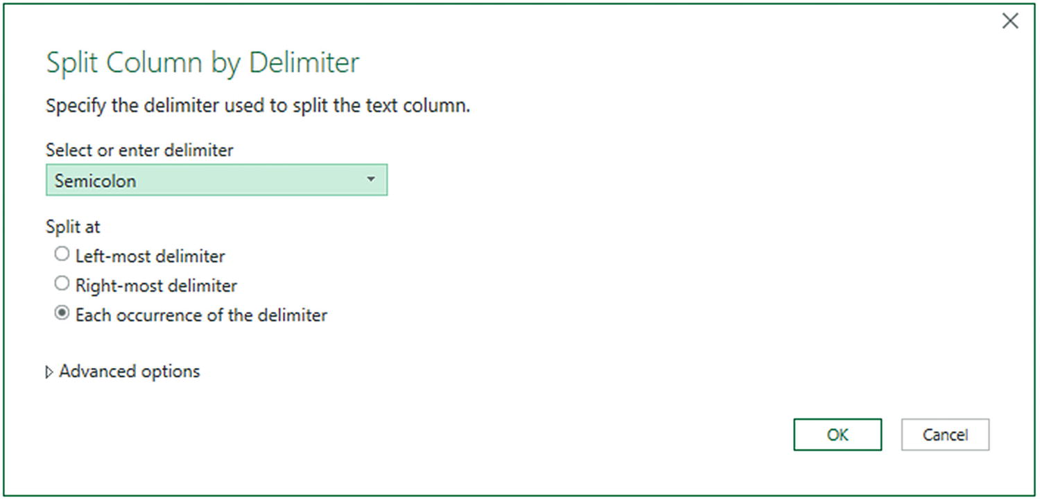
Splitting a column using a delimiter
- 11.
Click OK. Split Column by Delimiter will appear in the Applied Steps list.
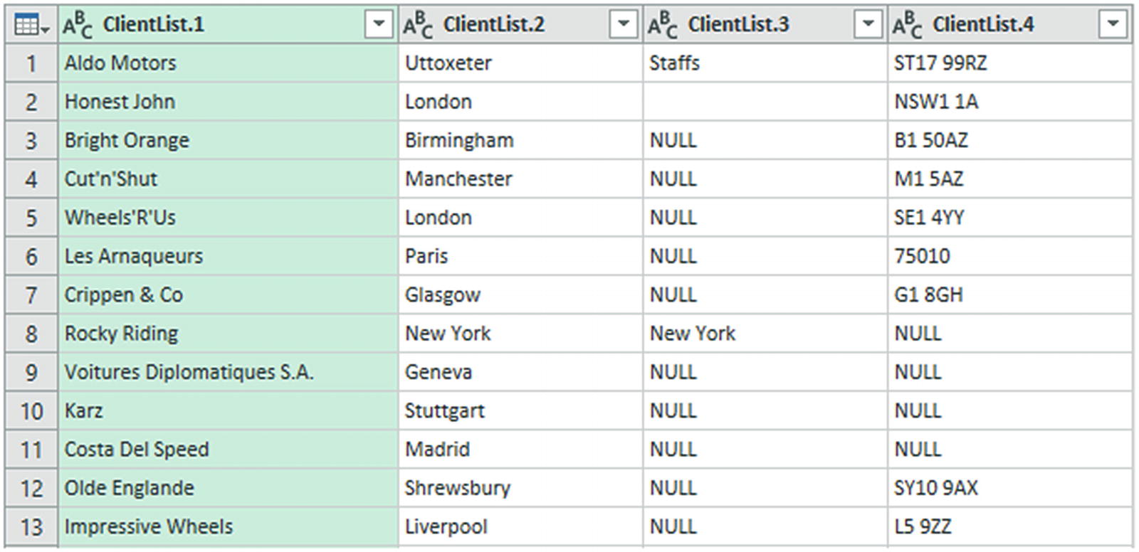
The results of splitting a column
Delimiter Split Options
Option | Description |
|---|---|
Colon | Uses the colon (:) as the delimiter |
Comma | Uses the comma (,) as the delimiter |
Equals Sign | Uses the equals sign (=) as the delimiter |
Semi-Colon | Uses the semicolon (;) as the delimiter |
Space | Uses the space ( ) as the delimiter |
Tab | Uses the tab character as the delimiter |
Custom | Lets you enter a custom delimiter |
At the Left-Most Delimiter | Splits the column once only at the first occurrence of the delimiter |
At the Right-Most Delimiter | Splits the column once only at the last occurrence of the delimiter |
At Each Occurrence of the Delimiter | Splits the column into as many columns as there are delimiters |
Split into Columns | This leaves the number of rows as it is in the dataset and creates new columns for each new element resulting from the split operation |
Split into Rows | Creates a new row for each new element resulting from the split operation and duplicates the existing record as many times as there are split elements |
Advanced Options for Delimiter Split
Delimiter Split Options
Advanced options ➤ Number of Columns to Split Into | Allows you to set a maximum number of columns into which the data is split in chunks of the given number of characters. Any extra columns are placed in the rightmost column |
Advanced options ➤ Quote Character | Separators inside a text that is contained in double quotes are not used to split the text into columns. Setting this option to “none” will split elements inside quotes |
Split using special characters | Enables the Insert Special Character button. You can then click this button and select the special character to split data on. The choice is between Tab, Carriage Return, Line-Feed, Carriage Return and Line-Feed, and Non-breaking Space |
Splitting Columns by Number of Characters
Options When Splitting a Column by Number of Characters
Option | Description |
|---|---|
Number of Characters | Lets you define the number of characters of data before splitting the column |
Once, As Far Left As Possible | Splits the column once only at the given number of characters in from the left (if the length of the data in the row allows this) |
Once, As Far Right As Possible | Splits the column once only at the given number of characters in from the right (if the length of the data in the row allows this) |
Repeatedly | Splits the column as many times as necessary to cut it into segments every defined number of characters |
Advanced options ➤ Number of Columns to Split Into | Allows you to set a maximum number of columns into which the data is split in chunks of the given number of characters. Any extra columns are placed in the rightmost column |
Split into Columns | This leaves the number of rows as it is in the dataset and crates new columns for each new element resulting from the split operation |
Split into Rows | Creates a new row for each new element resulting from the split operation and duplicates the existing record as many times as there are split elements |
When splitting by a delimiter, Power Query makes a good attempt at guessing the maximum number of columns into which the source column must be split. If it gets this wrong (and you can see what its guesstimate is if you expand the Advanced options box), you can override the number here.
If you select a Custom Delimiter, Power Query displays a new box in the dialog where you can enter a specific delimiter.
Not every record has to have the same number of delimiters. Power Query simply leaves the rightmost column(s) blank if there are fewer split elements for a row.
You can only split columns if they are text data. The Split Column button remains grayed out if your intention is to try to split a date or numeric column. You can, however, convert the data type from a date, datetime, or numeric data type to a text data type before splitting a column.
Merging Columns
You may be feeling a certain sense of déjà vu when you read the title of this section. After all, we saw how to merge columns (i.e., how to fuse the data from several columns into a single, wider column) in a previous chapter, did we not?
Yes, we did indeed. However, this is not the only time in this chapter that you will see something that you have tried previously. This is because Power Query repeats several of the options that are in the Transform ribbon in the Add Column ribbon. While these functions all work in much the same way, there is one essential difference. If you select an option from the Transform ribbon, then the column(s) that you selected is modified. If you select a similar option from the Add Column ribbon, then the original column(s) will not be altered, but a new column is added containing the results of the data transformation.
Merging columns is a case in point. Now, as I went into detail as to how to execute this kind of data transformation in the previous chapter, I will not describe it all over again here. Suffice it to say, if you Ctrl-click the headings of two or more columns and then click Merge Columns in the Add Column ribbon, you will still see the data from the selected columns concatenated into a single column. However, this time the original columns remain in the dataset. The new column is named Merged, exactly as was the case for the first of the columns that you selected when merging columns using the Transform ribbon.
Format: Trims or changes the capitalization of text
Extract: Takes part of a column and creates another column from this data
Parse: Adds a column containing the source column data as JSON or XML strings
Statistics: Creates a new column of aggregated numeric values
Standard: Creates a new column of calculated numeric values
Scientific: Creates a new column by applying certain kinds of math operations to the values in a column
Trigonometry: Creates a new column by applying certain kinds of trigonometric operations to the values in a column
Rounding: Creates a new column by rounding the values in a column
Information: Creates a new column indicating arithmetical information about the values in a column
Date: Creates a new column by extracting date elements from the values in a date column
Time: Creates a new column by extracting time elements from the values in a time or date/time column
Duration: Creates a new column by calculating the duration between two dates or date/times.
When transforming data, the art is to decide whether you want or need to keep the original column before applying one of these functions. Yet, once again, it is not really fundamental if you later decide that you made an incorrect decision, as you can always backtrack. Alternatively, you can always decide to insert new columns as a matter of principle and delete any columns that you really do not need at a later stage in the data transformation process.
Creating Columns from Examples
Creating your own columns can be a little scary if you have not had much previous experience with Excel or Power Pivot formulas, so the Power Query development team has tried to make your life easier by adding another way to create custom columns. Instead of referring to columns by the column name (and having to handle square brackets and other peculiar characters), you can build a new column by using the actual data in a row.
- 1.
Load the C:DataMashupWithExcelSamplesChapter07Example1.xlsx sample file.
- 2.
Display the Queries & Connections pane if necessary by clicking Queries & Connections in the Data ribbon.
- 3.
Double-click the BaseData query to switch to the Query Editor.
- 4.
In the Add Column ribbon, click Column From Examples. A new kind of formula bar will appear above the data. It will look like Figure 7-20. At the same time, a new, empty column will be created at the right of the existing data.
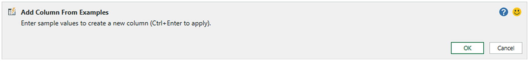
Creating a column from examples
- 5.
Double-click the new column on the right. A list of data from each field will be displayed, as shown in Figure 7-21.
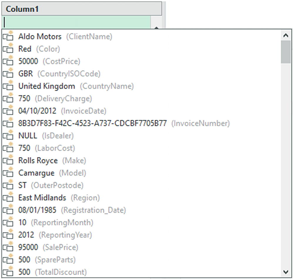
Displaying the data from a row when creating a column from examples
- 6.
Double-click Red to select the data from the Color column.
- 7.
Enter a space, a hyphen, and a space, then type Camargue (this is the name of the model for this row).
- 8.
Click OK in the formula bar at the top.
Power Query will add a new column containing the color, a separator, and the Model. Inserted Merged Column will be added as a new step in the Applied Steps list. In fact, what Power Query has done is to use the column contents as a proxy for the column name.
In the popup menu for the Column from Examples button, you can choose to take all existing columns as the basis for the example or only any columns that you have previously selected.
As you can see from this short example, creating columns by example lets you use the data from a column rather than the column name. It also removes the need for double quotes and ampersand characters that you had to use when writing the code to create a new column in the previous section.
If you select Column From Examples ➤ From Selection, then you will only see data from the selected columns when you double-click inside the new column to see samples of data as you did in step 6 of this example.
Adding Conditional Columns
Not all additional columns are a simple extraction or concatenation of existing data. There will be times when you will want to apply some simple conditions that define the contents of a new column. This is where Power Query’s Conditional Column function comes into its own.
- 1.
Load the C:DataMashupWithExcelSamplesChapter07Example1.xlsx sample file.
- 2.
Display the Queries & Connections pane (if required) by clicking Queries & Connections in the Data ribbon.
- 3.
Double-click the BaseData query to switch to the Query Editor.
- 4.
In the Add Column ribbon, click Conditional Column. The Add Conditional Column dialog will appear.
- 5.
Enter BuyerType in the “New column name” field.
- 6.
Select Make as the column name.
- 7.
Leave equals as the operator.
- 8.
Enter Rolls Royce as the value.
- 9.
Enter Posh as the output.
- 10.
Click Add Clause.
- 11.
Select Make as the column name, leave equals as the operator, enter Bentley as the value, and add Classy as the output.
- 12.
Enter Bling in the Else field. The dialog will look like Figure 7-22.
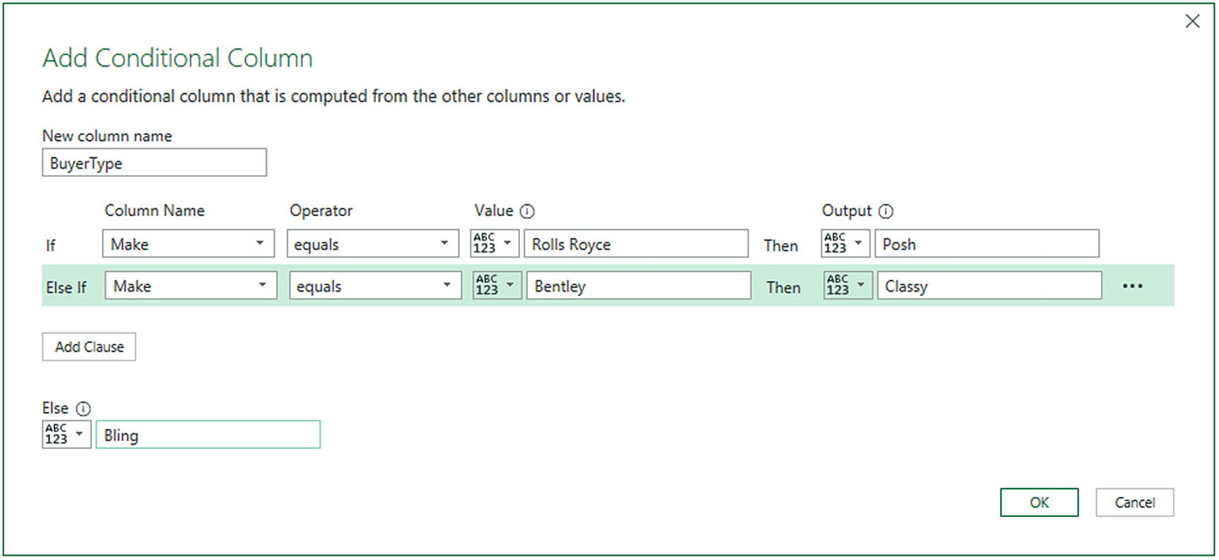
The Add Conditional Column dialog
- 13.
Click OK. The new column will be added containing either Posh, Classy, or Bling, depending on the make for each record. Added Conditional Columns will appear as the new step in the Applied Steps list.
Custom Column Operators
Operator | Description |
|---|---|
Equals | Sets the text that must match the contents of the selected field for the output to be applied |
Does Not Equal | Sets the text that must not match the contents of the selected field for the output to be applied |
Begins With | Sets the text at the left of the selected field for the output to be applied |
Does Not Begin With | Sets the text that must not appear at the left of the selected field for the output to be applied |
Ends With | Sets the text at the right of the selected field for the output to be applied |
Does Not End With | Sets the text that must not appear at the right of the selected field for the output to be applied |
Contains | Sets the text that can appear anywhere in the selected field for the output to be applied |
Does Not Contain | Sets the text that cannot appear anywhere in the selected field for the output to be applied |
It is also worth noting that the comparison value, the output, and the alternative output can be values (as was the case in this example), columns, or parameters (which you will learn about in Chapter 9). If you want to remove a rule, simply click the ellipses at the right of the required rule and select Delete.
Should you wish to alter the order of the rules in the Add Conditional Column dialog, all you have to do is click the ellipses at the right of the selected rule and select Move Up or Move Down from the popup menu.
Index Columns
Reapply a previous sort order.
Create a unique reference for every record.
Prepare a recordset for use as a dimension table in a Power Pivot data model. In cases like this, the index column becomes what dimensional modelers call a surrogate key .
- 1.
In the Add Column ribbon, click Index Column. The new, sequentially numbered column is added at the right of the table, and Added Index is added to the Applied Steps list.
- 2.
Scroll to the right of the table and rename the index column; it is currently named Index.
Start at 0 and increment by a value of 1 for each row.
Start at 1 and increment by a value of 1 for each row.
Start at any number and increase by any number.
As you saw when adding Index columns, the default is for Power Query to begin numbering rows at 0. However, you can choose another option by clicking the small triangle to the right of the Add Index Column button. This displays a menu with the three options outlined.

The Add Index Column dialog
This dialog lets you specify the start number for the first row in the dataset as well as the increment that is added for each record.
Conclusion
In this chapter, you learned some essential techniques that you can use to cleanse and structure datasets. You saw how to round numbers up and down, how to deliver conformed text presentation, and how to remove extraneous spaces and nonprinting characters from columns of data.
You also saw how to replace values inside columns, as well as ways of applying mathematical, statistical, and trigonometric functions to numbers. Other techniques covered extracting date, time, and duration elements from date/time and duration columns.
Finally, you saw a series of techniques that help you to add new columns based on the data in existing columns. These range from simple copies of an entire column or combining columns to extracting parts of a column’s data or even deducing different data that is added to a new column using simple logic.
It is now time to see how you can join hitherto separate datasets into single queries and parse complex data types to add them to a dataset. You will even learn how to append multiple files in a single query and how to pivot and unpivot data. All of this will be the subject of the next chapter.