Not all data loads are a matter of simply establishing a connection and applying transformations to the source data that is, fortunately, already laid out in neatly structured tables. Sometimes you may want to “push the envelope” when loading data and prepare more complex source data structures for use in your Excel analytics. By this, I mean that the source data is not initially in a ready-to-use tabular format and that some restructuring of the data is required to prepare a clean table of data for use.
Add multiple identical files from a source folder
Select the identical source files to load from a source folder
Load simple JSON structures from a source file containing JSON data
Parse a column containing JSON data in a source file
Parse a column containing XML data in a source file
Load complex JSON files—and select the elements to use
Load complex XML files—and select the elements to use
Convert columns to lists for use in complex load routines
Reuse recently used queries
Modify the list of recently used queries
Export data from the Power Query Editor
Any sample files used in this chapter are available for download from the Apress website as described in Appendix A.
Adding Multiple Files from a Source Folder
Now let’s consider an interesting data ingestion challenge. You have been sent a collection of text files, possibly downloaded from an FTP site or received by email, and you have placed them all into a specific directory. However, you do not want to have to carry out the process that you saw in Chapter 2 and load files one by one if there are several hundred files—and then append all these files individually to create a final composite table of data (as you saw in Chapter 8).
Here is a much more efficient method to achieve this objective.
Query Editor can only load multiple files if all the files are rigorously identical. This means ensuring that all the columns are in the same order in each file and have the same names.
- 1.
Create a new Excel file.
- 2.
In the Data ribbon, click Get Data ➤ From File ➤ From Folder. The Folder dialog is displayed.
- 3.
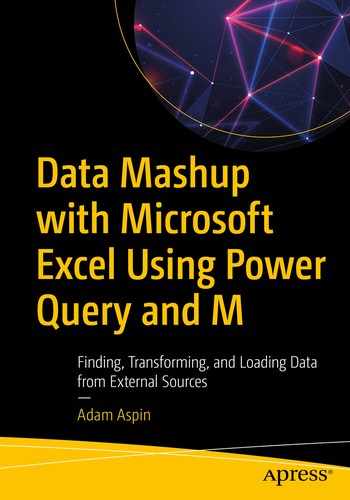
Click the Browse button and navigate to the folder that contains the files to load. In this example, it is C:DataMashupWithExcelSamplesMultipleIdenticalFiles. You can also paste in, or enter, the folder path if you prefer. The Folder dialog will look like Figure 9-1.
The Folder dialog
- 4.
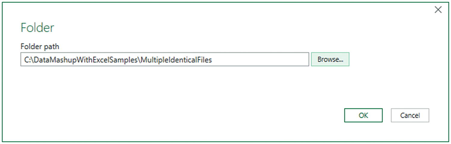
Click OK. The file list window opens. The contents of the folder and all subfolders are listed in tabular format, as shown in Figure 9-2.
The folder contents in Power Query
- 5.
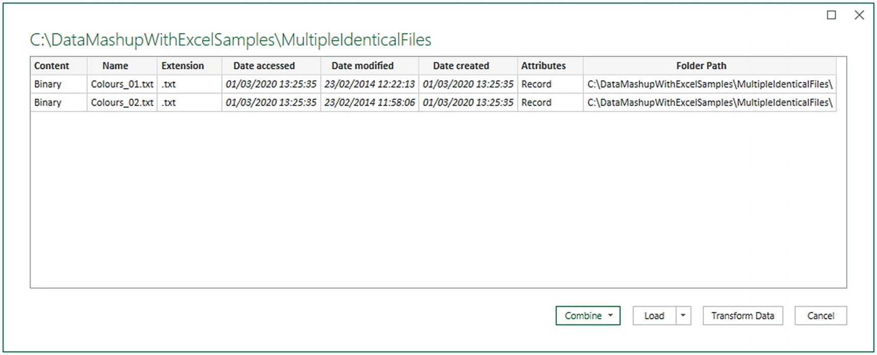
Click the popup arrow on the right of the Combine button and select Combine & Transform Data. The Combine Files dialog will appear, as shown in Figure 9-3. Here you can select which of the files in the folder is the model for the files to be imported.
The Combine Files dialog
- 6.
Click OK. The Power Query Editor will display the imported data. This is shown in Figure 9-4.
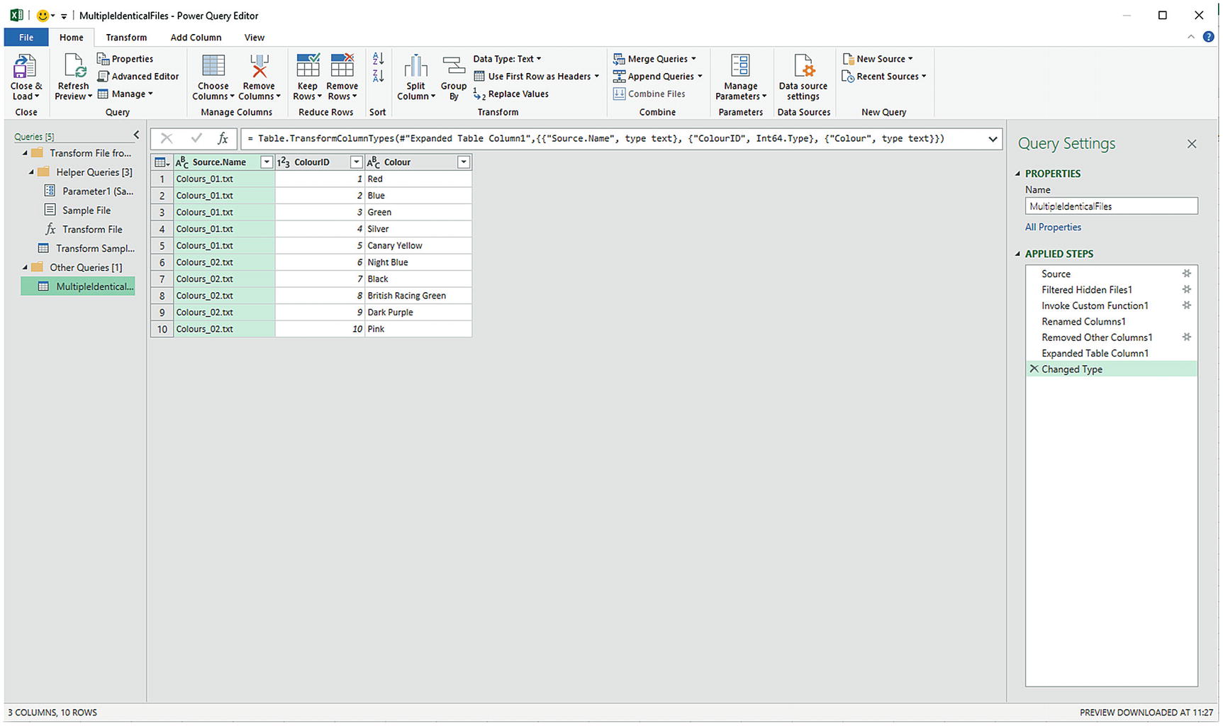
Data loaded from a folder
- 7.
Click Close & Load. The data from all the source files will be loaded into the Excel data model.
As you can see, Power Query has added an extra column to the output containing the name of the file that contained each source record. You can remove this column if you wish.
The other options in the Combine Files dialog are explained in Chapter 2.
Filtering Source Files in a Folder
There will be times when you want to import only a subset of the files from a folder. Perhaps the files are not identical or maybe you simply do not need some of the available files in the source directory. Whatever the reason, here is a way to get Power Query to do the work of trawling through the directory and only loading files that correspond to a file name or extension specification you have indicated, for instance. In other words, the Query Editor allows you to filter the source file set before loading the actual data. In this example, I will show you how to load multiple Excel files from a directory containing both Excel and text files.
- 1.
Carry out steps 1 through 5 from the section “Adding Multiple Files from a Source Folder” earlier in this chapter to display the contents of the folder containing the files you wish to load. In this scenario, it is C:DataMashupWithExcelSamplesMultipleNonIdentical.
- 2.
Click Transform Data. The Query Editor window will open and display the list of files in the directory and many of their attributes. You can see an example of this in Figure 9-5.
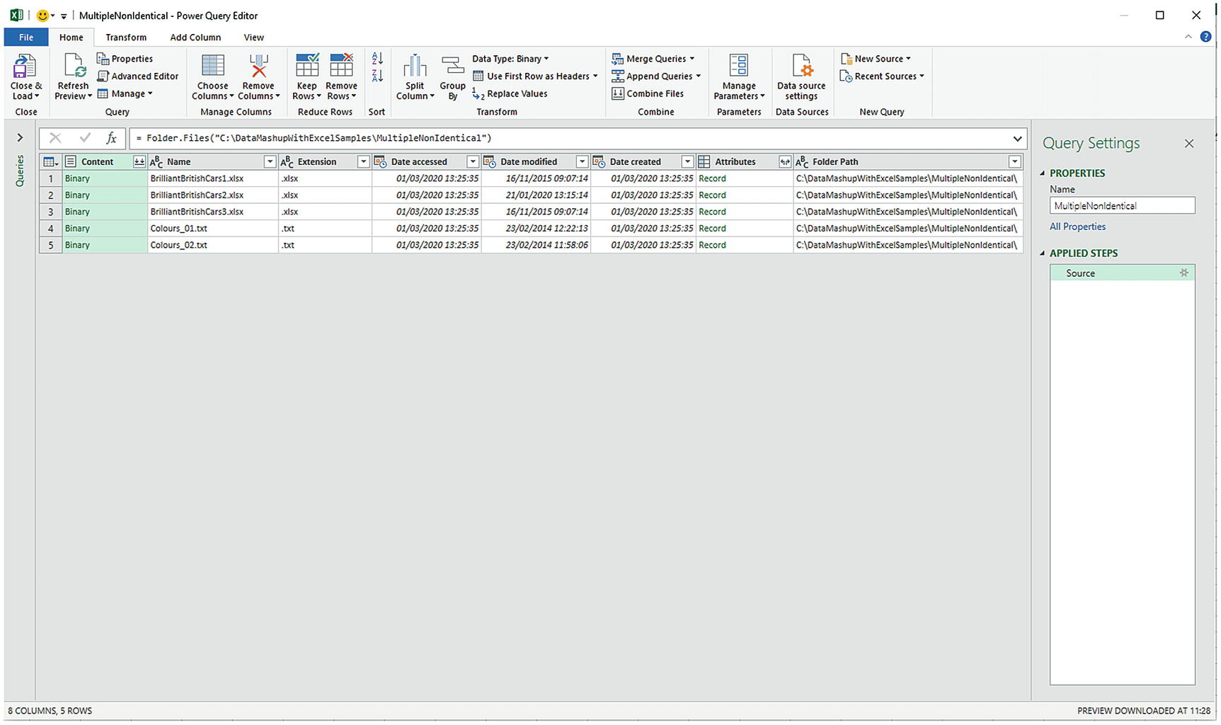
Displaying file information when loading multiple files
- 3.
As you want to load only Excel files, and avoid files of any other type, click the filter popup menu for the column title Extension and uncheck all elements except .xlsx. This is shown in Figure 9-6.
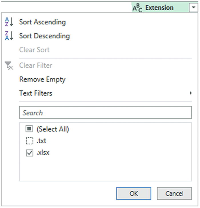
Filtering file types when loading multiple identical files
- 4.
Click OK. You will now only see the Excel files in the Query Editor.
- 5.
Click the Expand icon (two downward-facing arrows) to the right of the first column title; this column is called Content, and every row in the column contains the word Binary. Power Query will display the Combine Files dialog that you saw previously in Figure 9-3.
- 6.
Select the file from those available that you want to use as the sample file for the data load.
- 7.
Select the BaseData worksheet as the structure to use for the load.
- 8.
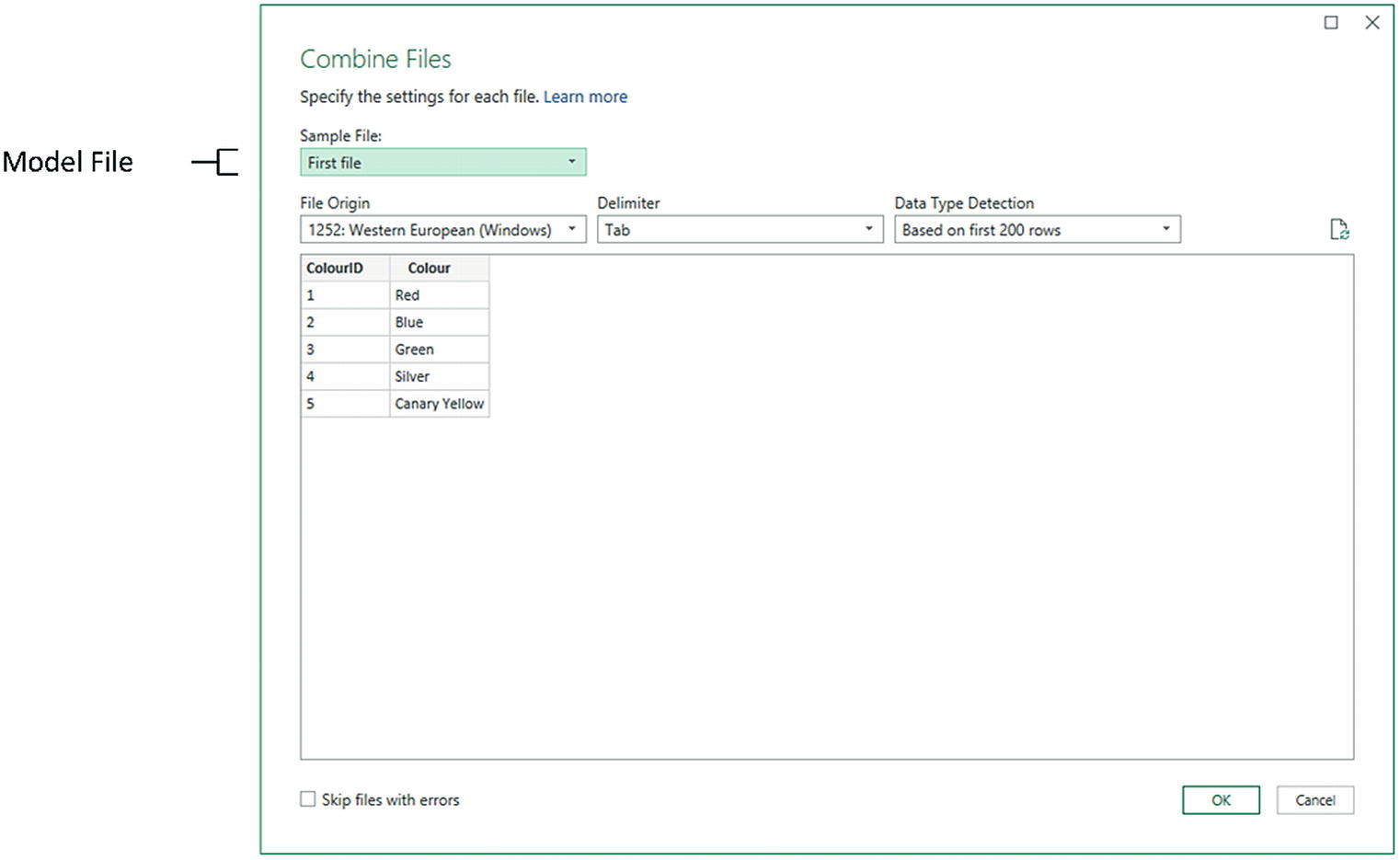
Click Skip files with errors. This time, the dialog will look like Figure 9-7.
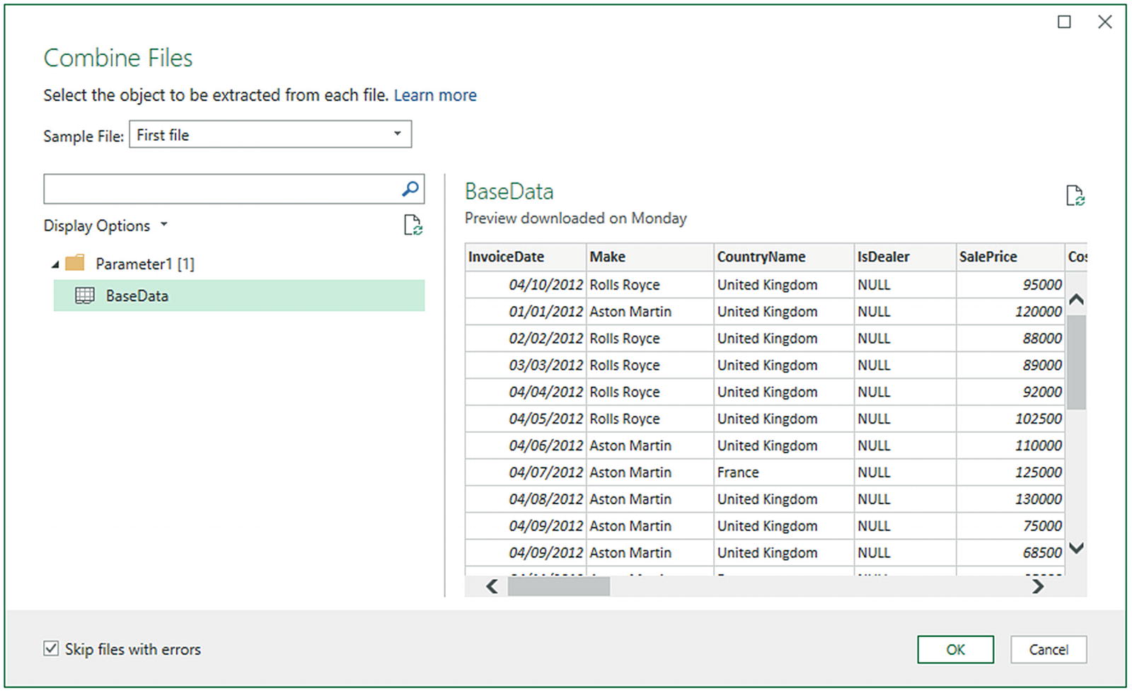
Selecting the source data when loading multiple Excel files
- 9.
Click OK. Power Query Editor will load all the files and display the result.
The contents of all the source files are now loaded into the Power Query Editor and can be transformed and used like any other dataset. This might involve removing superfluous header rows (as described in the next but one section). What is more, if ever you add more files to the source directory, and then click Refresh in the Home ribbon, all the source files that match the filter selection are reloaded, including any new files added to the specified directory since the initial load that match the filter criteria.
When loading multiple Excel files, you need to be aware that the data sources (whether they are worksheets, named ranges, or tables) must have the same name in all the source files or the data will not be loaded.
Displaying and Filtering File Attributes
File name
File extension
Folder path
Date created
Date last accessed
Date modified
- 1.
Carry out steps 1 and 2 from the previous section.
- 2.
Display the available attributes by clicking the expand icon (the double-headed arrow) at the right of the attribute column. The list of available attributes will be displayed, as shown in Figure 9-8.
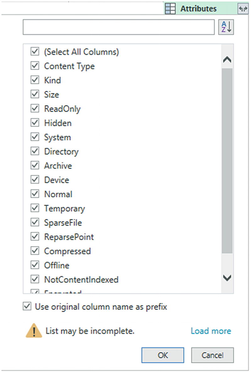
Adding file attributes for file selection
- 3.
Select the attributes that you want to display from the list and click OK.
Each attribute will appear as a new column in the Query Editor. You can now filter on the columns to select files based on the expanded list of attributes.
You can also filter on directories, dates, or any of the file information that is displayed. Simply apply the filtering techniques that you learned in Chapter 6.
Removing Header Rows After Multiple File Loads
- 1.
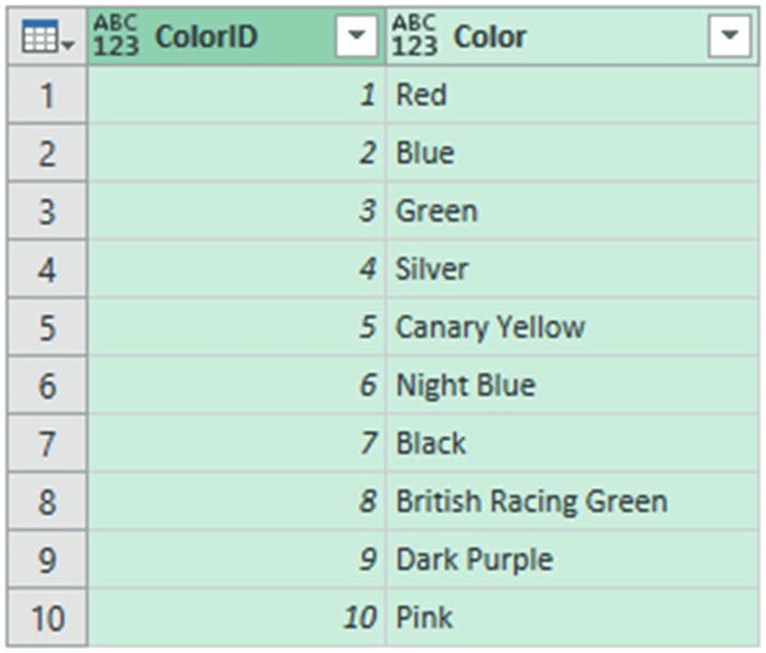
If (but only if) each file contains header rows, then scroll down through the resulting table until you find a title element. In this example, it is the word ColourID in the ColourID column.
- 2.
Right-click ColourID and select Text Filters ➤ Does Not Equal. All rows containing superfluous column titles are removed.
If your source directory only contains the files that you want to load, then step 2 is unnecessary. Nonetheless, I always add steps like this in case files of the “wrong” type are added later, which would cause any subsequent process runs to fail. Equally, you can set filters on the file name to restrict the files that are loaded.
Combining Identically Structured Files
- 1.
Carry out steps 1 through 5 in the section “Adding Multiple Files from a Source Folder” to display the contents of the folder containing the files you wish to load. In this scenario, it is C:DataMashupWithExcelSamplesMultipleIdenticalFiles.
- 2.
Click the column named Content.
- 3.
In the Power Query Home ribbon, click the Combine Files button. The Combine Files dialog (that you saw in Figure 9-7) will appear.
- 4.
Click OK.
Power Query will evaluate the format of the source files and append all the source files into a single query.
Power Query will create a set of helper queries to carry out this operation. If you expand the Power Query Queries pane, you will see the new queries that it has added. These queries will also be displayed in the Excel Queries & Connections pane.
Loading and Parsing JSON Files
More and more data is now being exchanged in a format called JSON. This stands for JavaScript Object Notation, and it is considered an efficient and lightweight way of transferring potentially large amounts of data. A JSON file is essentially a text file that contains data structured in a specific way.
Now, while Power Query can connect very easily to JSON data files (they are only a kind of text file, after all), the data they contain are not always instantly comprehensible. So you will now learn how to load the file and then see how this connection can be tweaked to convert it into meaningful information. Transforming the source text into a comprehensible format is often called parsing the data.
- 1.
In the Data ribbon, click Get Data ➤ From File ➤ From JSON.
- 2.
Select the file C:DataMashupWithExcelSamplesColors.json, and click Import. You will see a list of records like the one shown in Figure 9-9.
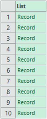
A JSON file after initial import
- 3.
You will see that the Query Editor has added the List Tools Transform ribbon to the menu bar. This ribbon is explained in detail in the next section. Click the To Table button in this ribbon. The To Table dialog will appear, as shown in Figure 9-10.
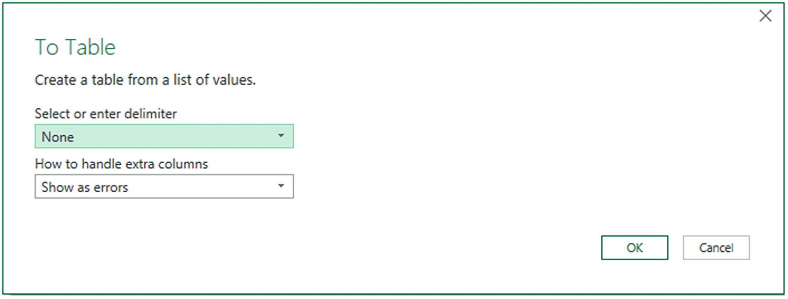
The To Table dialog
- 4.
Click OK. The list of data will be converted to a table. This means that it now shows the Expand icon at the right of the column title, as you can see in Figure 9-11.
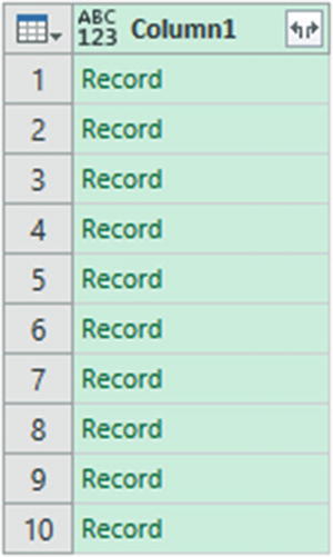
A JSON file converted to a table
- 5.
Click the Expand icon to the right of the column title, and in the popup dialog, uncheck “Use original column name as prefix.”
- 6.
Click OK. The contents of the JSON file now appear as a standard dataset, as you can see in Figure 9-12.
A JSON file transformed into a dataset
Although not particularly difficult, this process may seem a little counterintuitive. However, it certainly works, and you can use it to process complex JSON files so that you can use the data they contain in Excel.
The List Tools Transform Ribbon
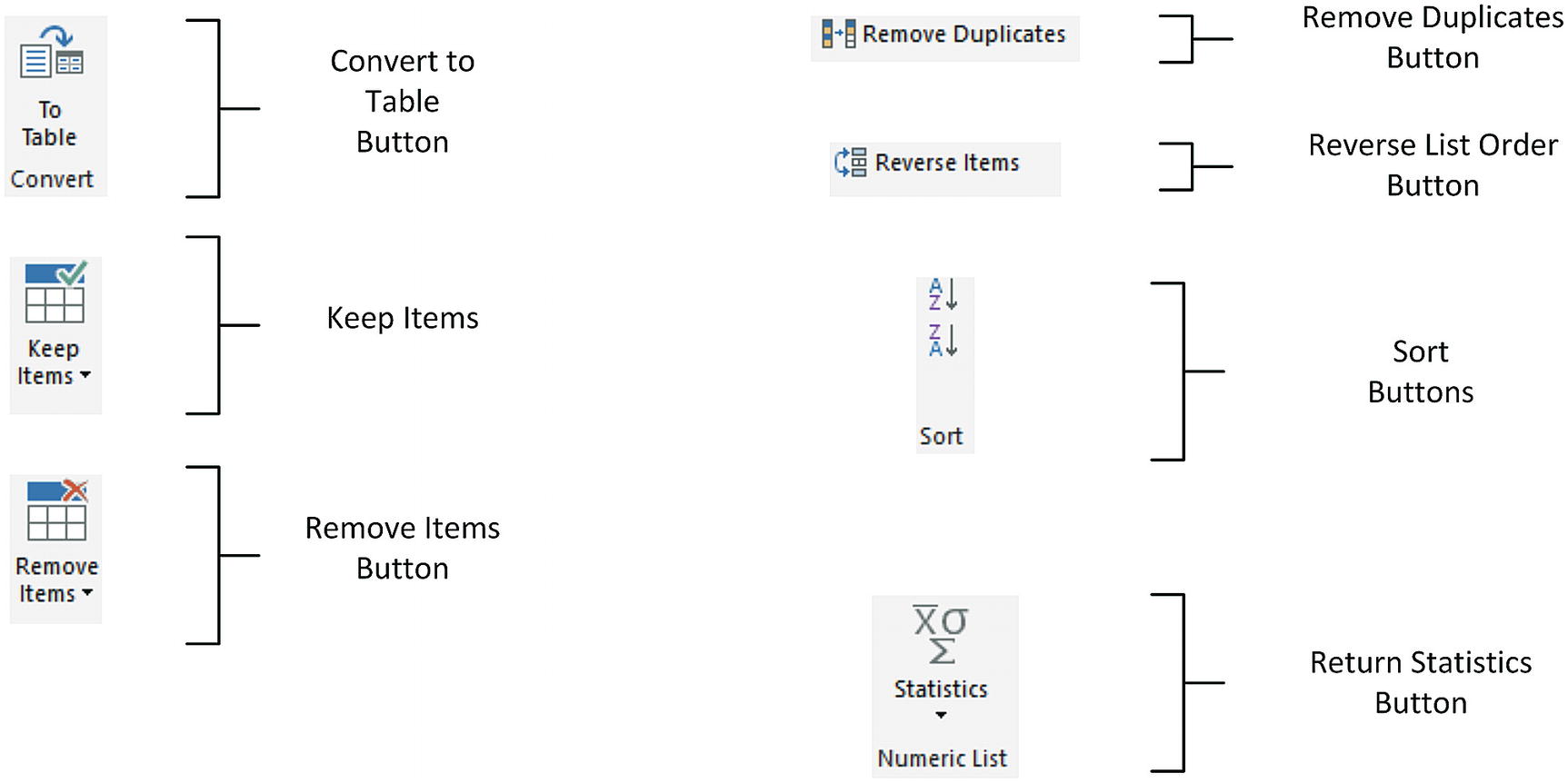
The List Tools Transform ribbon
The List Tools Transform Ribbon Options
Option | Description |
|---|---|
To Table | Converts the list to a table structure |
Keep Items | Allows you to keep a number of items from the top or bottom of the list or a range of items from the list |
Remove Items | Allows you to remove a number of items from the top or bottom of the list or a range of items from the list |
Remove Duplicates | Removes any duplicates from the list |
Reverse Items | Reverses the list order |
Sort | Sorts the list lowest to highest or highest to lowest |
Statistics | Returns calculated statistics about the elements in the list |
Parsing XML Data from a Column
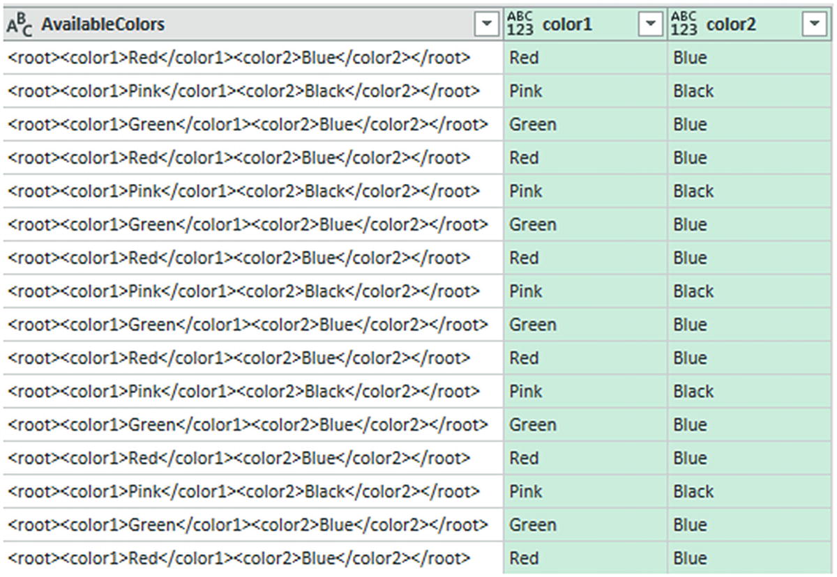
Some data sources, particularly database sources, include XML data actually inside a field. The problem here is that XML data is interpreted as plain text by Power Query when the data is loaded. If you look at the AvailableColors column that is highlighted in Figure 9-14, you can see that this is not particularly useful or even comprehensible.
- 1.
In the Data ribbon, click Get Data ➤ From File ➤ From Workbook.
- 2.
Select the file XMLInColumn.xlsx and click Import.
- 3.
Select the Sales table on the left of the Navigator and click Transform Data to switch to the Query Editor.
- 4.Scroll to the right of the dataset and select the last column: AvailableColors. The Query Editor looks like Figure 9-14.
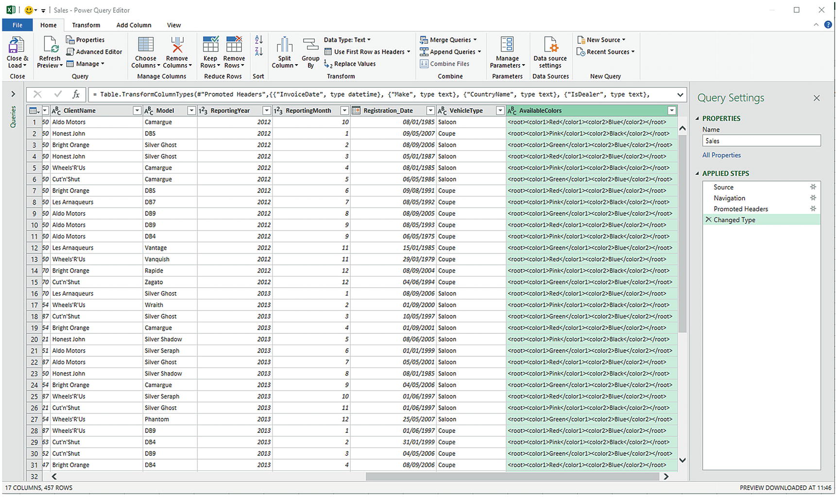 Figure 9-14
A column containing XML
- 5.
In the Add Column ribbon, click the small triangle in the Parse button and select XML. A new column will be added to the right. It will look like Figure 9-15 and will have the title XML.
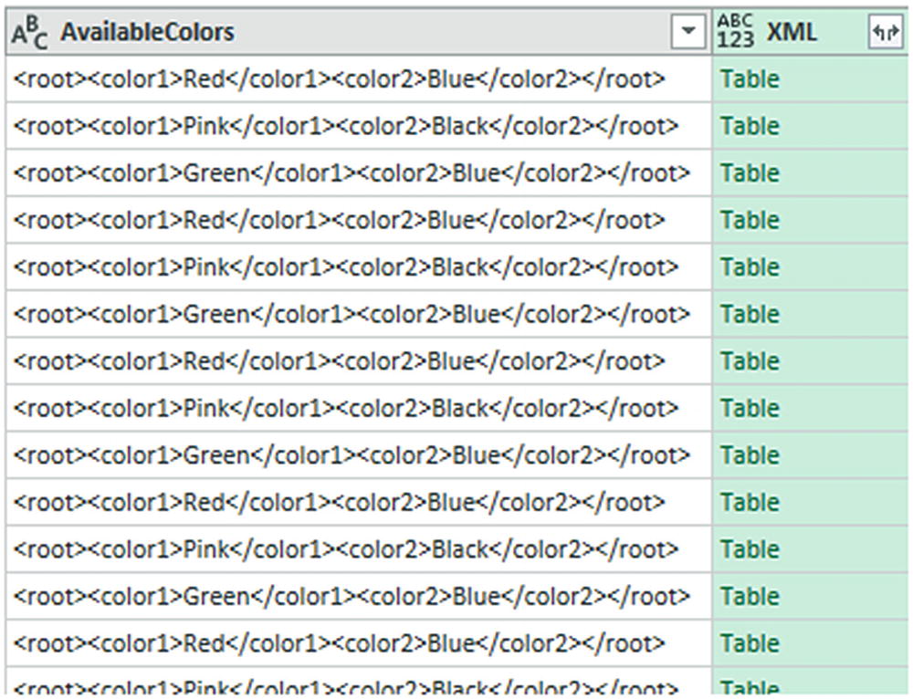
An XML column converted to a table column
- 6.
Click the Expand icon to the right of the XML column title and uncheck “Use original column name as prefix” in the popup dialog. Ensure that all the columns are selected and click OK. Two new columns (or, indeed, as many new columns as there are XML data elements) will appear at the right of the dataset. The Query Editor will look like Figure 9-16.
XML data expanded into new columns
- 7.
Remove the column containing the initial XML data by selecting the column that contains the original XML and clicking Remove columns in the context menu.
- 8.
Rename any new columns to give them meaningful titles.
Using this technique, you can now extract the XML data that is in source datasets and use it to extend the original source data.
Parsing JSON Data from a Column
Sometimes you may encounter data containing JSON in a field, too. The technique to extract this data from the field inside the dataset and convert it to columns is virtually identical to the approach that you saw in the previous section for XML data.
- 1.
Follow steps 1 through 4 from the previous example, only use the file C:DataMashupWithExcelSamplesJSONInColumn.xlsx. Select the only worksheet in this file: Sales.
- 2.
Scroll to the right of the dataset and select the last column: AvailableColors.
- 3.
In the Add Column ribbon, click Parse ➤ JSON. A new column will be added to the right and will have the title JSON.
- 4.
Click the Expand icon to the right of the JSON column title and uncheck “Use original column name as prefix” in the popup dialog. Ensure that all the columns are selected and click OK. Two new columns (or, indeed, as many new columns as there are JSON data elements) will appear at the right of the dataset. The Query Editor will look like Figure 9-17.
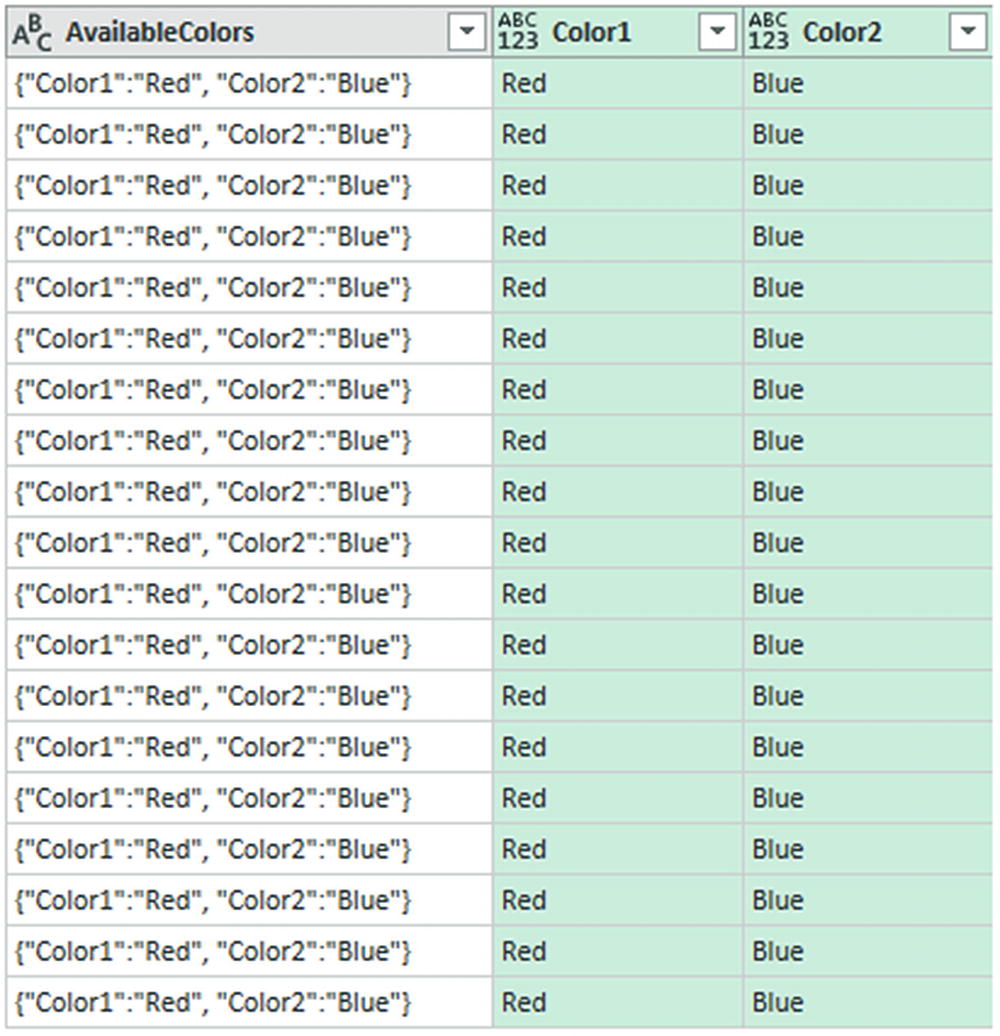
JSON data expanded into new columns
- 5.
Delete the column containing the initial JSON data.
- 6.
Rename any new columns if this is necessary.
Admittedly, the structure of the JSON data in this example is extremely simple. Real-world JSON data could be much more complex. However, you now have a starting point upon which you can build when parsing JSON data that is stored in a column of a dataset.
Complex JSON Files
JSON files are not always structured as simplistically as the Colors.json file that you saw a few pages ago. Indeed, JSON files can contain many sublevels of data, structured into separated nodes. Each node may contain multiple data elements grouped together in a logical way. Often you will want to select “sublevels” of data from the source file—or perhaps only select some sublevel elements and not others.
The vehicle
The finance data
The customer
The challenge here will be to “flatten” the data from the Vehicle and FinanceData nodes into standard columns that can then be used for analytics.
If you want to get an idea of what a complex JSON file containing several nested nodes looks like, then simply open the file C:DataMashupWithExcelSamplesCarSalesJSON_Complex.json in a text editor.
- 1.
In the Excel ribbon, click Get Data ➤ From File ➤ From JSON. Navigate to the folder containing the JSON file that you want to load (C:DataMashupWithExcelSamplesCarSalesJSON_Complex.json, in this example).
- 2.
Click Import. The Query Editor window will appear and automatically display the Record Tools Convert ribbon. You can see this in Figure 9-18.
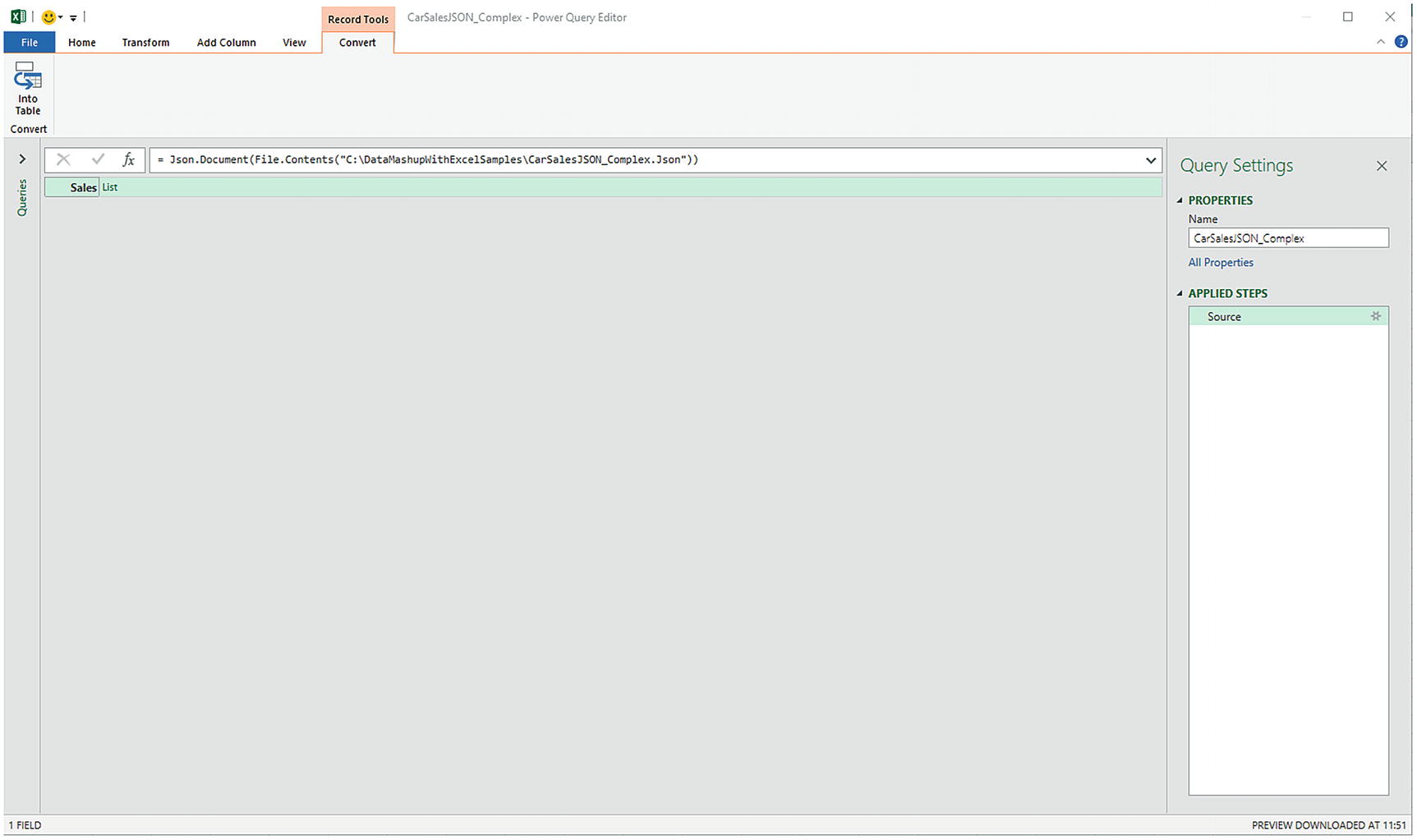
Opening a complex JSON file
- 3.
Click Into Table from the Record Tools Convert ribbon. The Query Editor will look like Figure 9-19.
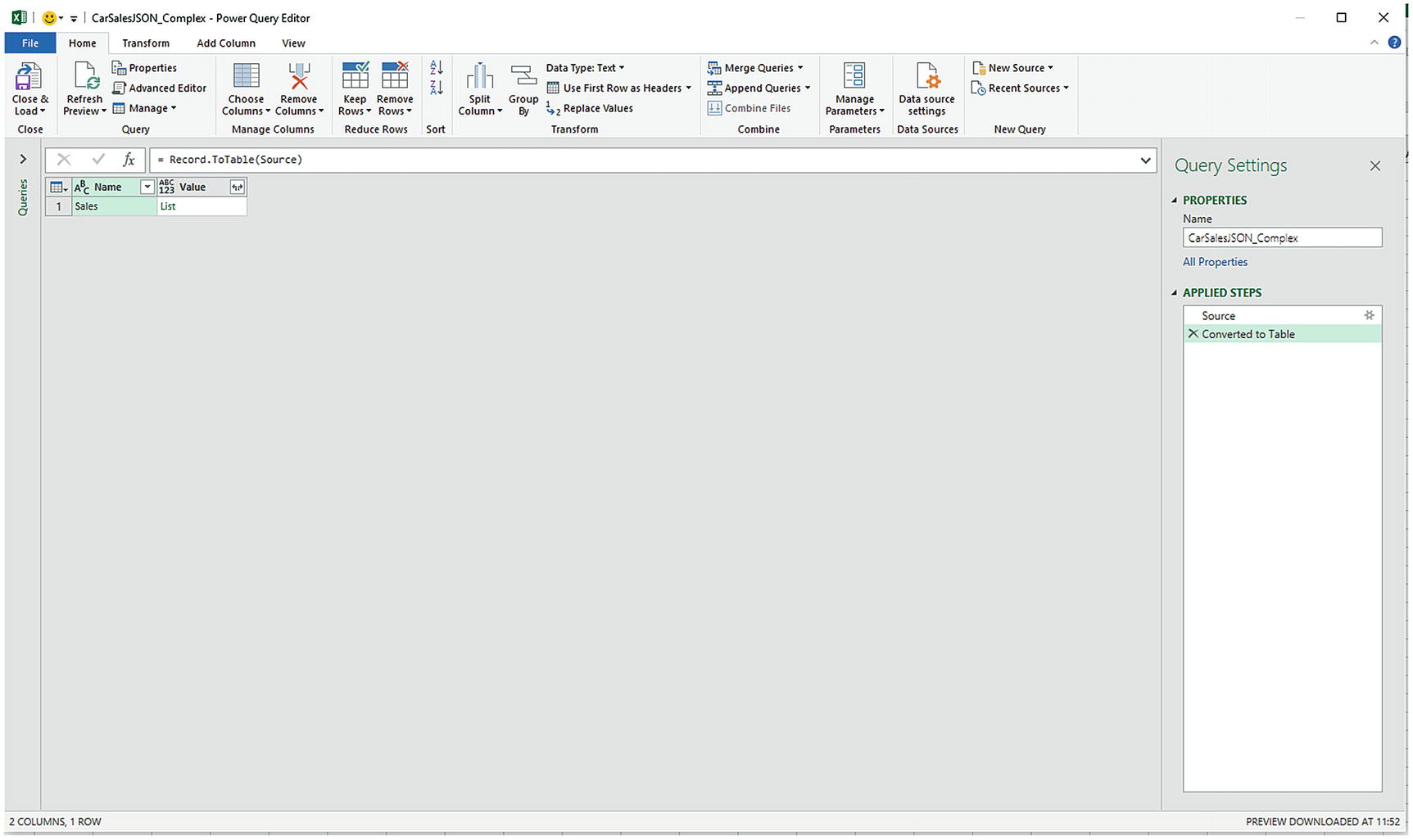
A complex JSON file
- 4.
Click the Expand icon at the top right of the Value column and select Expand to new rows. The Query Editor will look like Figure 9-20.
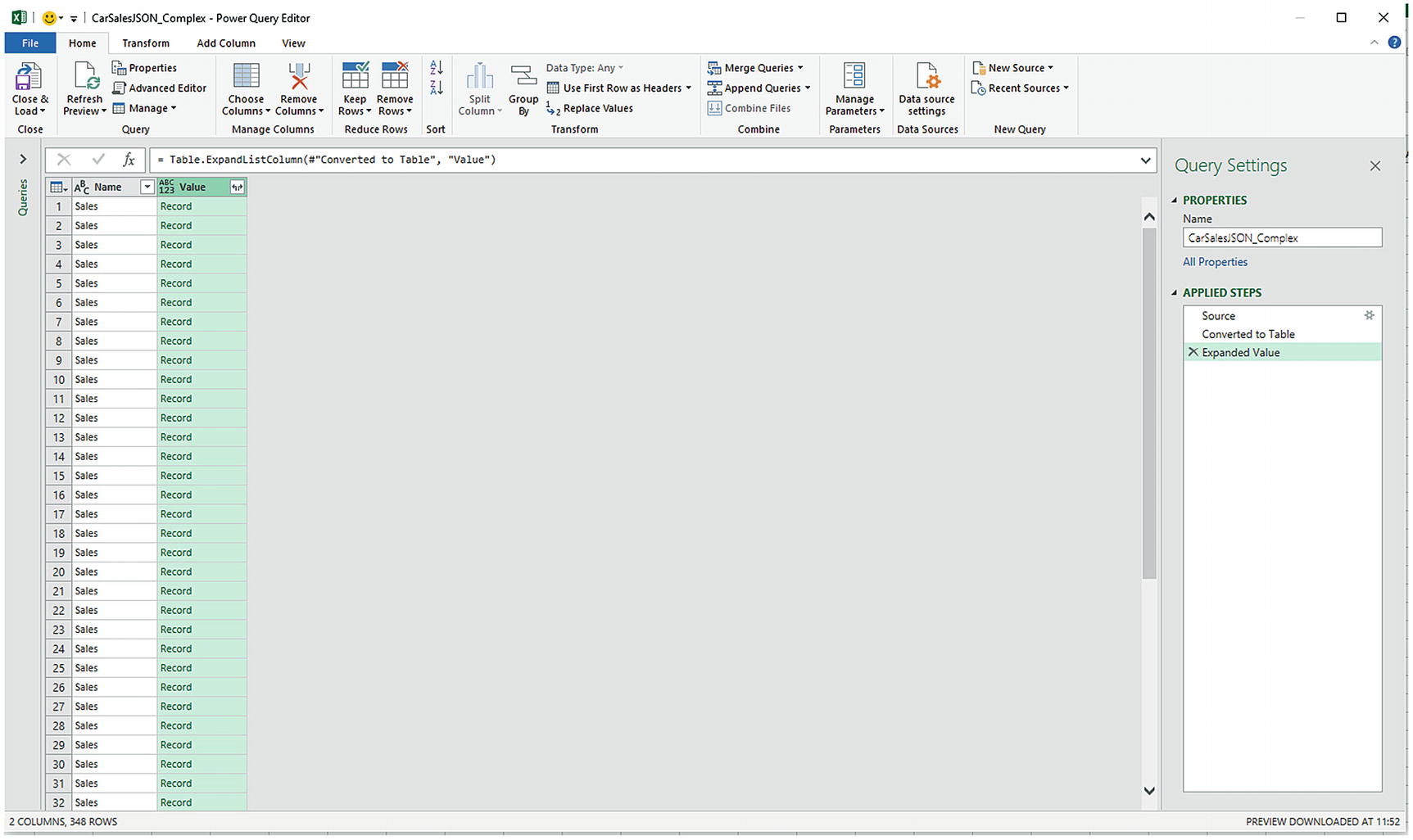
Expanding a JSON file
- 5.
Click the Expand icon at the top right of the Value column and uncheck Use original column name as prefix.
- 6.
Click OK to display all the JSON attributes. The Query Editor window will look like Figure 9-21. Each column containing the word “record” is, in fact, a JSON node that contains further sublevels of data.
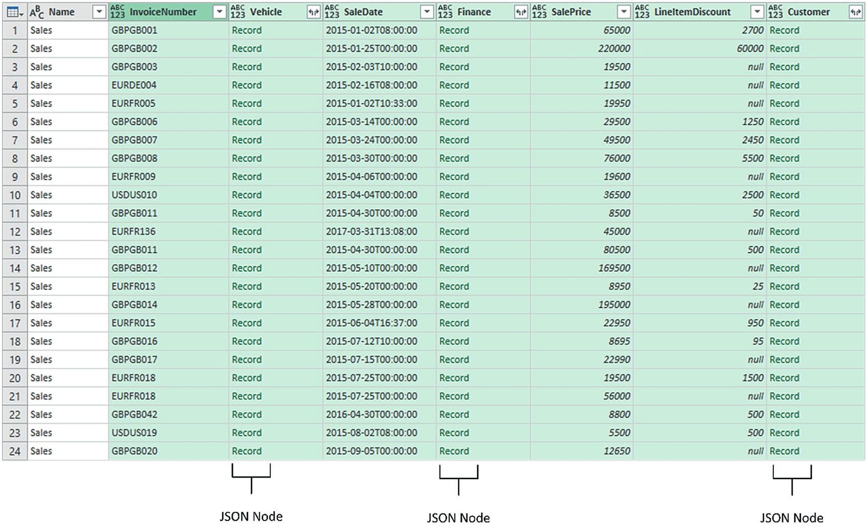
Viewing the structure of a JSON file
- 7.
Select the Vehicle column and click the Expand icon at the right of the column title. The list of available elements that are “nested” at a lower level inside the source JSON will appear. You can see this in Figure 9-22.
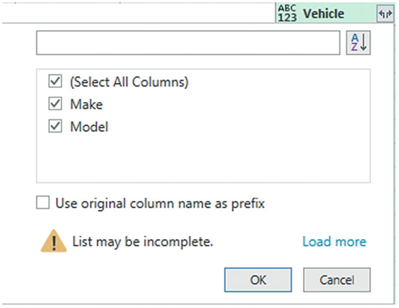
Nested elements in a JSON file
- 8.
Click OK. The new columns will be added to the data table.
- 9.
Select the Finance column and click the Expand icon at the right of the column title. The list of available elements that are “nested” at a lower level inside the source JSON for this column will appear. Select only the Cost column and click OK.
- 10.
Remove the Customer column as we will not be using data from this column in this example. The Query Editor window will look like Figure 9-23, where all the required columns are now visible in the data table.
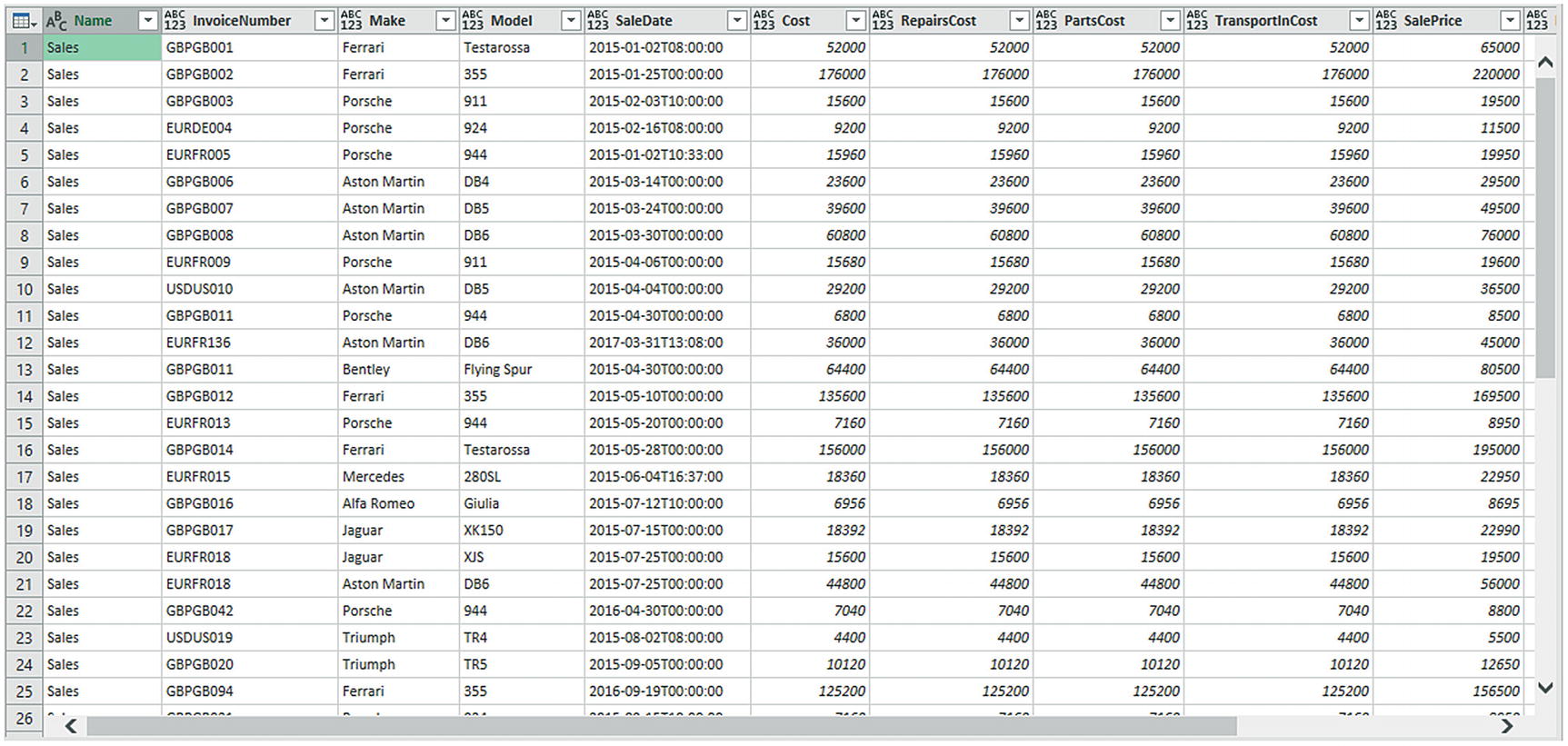
A JSON file after parsing
- 11.
Click the Close & Load in the Power Query Home menu to return the “flattened” JSON data to an Excel worksheet.
It is a good idea to click the Load more link in the Expand popup menu when you are identifying the nested data in a JSON node. This will force Power Query to scan a larger number of records and return, potentially, a more complete list of nested fields.
This approach allows you to be extremely selective about the data that you load from a JSON file. You can choose to include any column at any level from the source structure. As you saw, you can select—or ignore—entire sublevels of nested data extremely easily.
This section was only a simple introduction to parsing complex JSON files. As this particular data structure can contain multiple sublevels of data, and can mix data and sublevels in each node of the JSON file, the source data structure can be extremely complex and can contain nodes within nodes within nodes. Fortunately, the techniques that you just learned can be extended to handle any level of JSON complexity and help you tame the most potentially daunting data structures.
It is important to “flatten” the source data so that all the sublevels (or nodes if you prefer) are removed, and the data that they contain is displayed as a simple column in the query. Otherwise, the data will not be easy to use in Excel.
Complex XML Files
As is the case with JSON files, XML files can comprise complex nested structures of many sublevels of data, grouped into separate nodes. The good news is that the Power Query Editor handles both these data structures in the same way.
- 1.
In the Excel ribbon, click Get Data ➤ From File ➤ From XML. Navigate to the folder containing the XML file that you want to load (C:DataMashupWithExcelSamplesComplexXML.xml, in this example).
- 2.
Click Import. The Navigator dialog will appear.
- 3.
Select Sales as the source data table on the left.
- 4.
Click Transform Data. The Query Editor will appear.
- 5.
Select the Vehicle column and click the Expand icon at the right of the column title. The list of available elements that are “nested” at a lower level inside the source XML will appear.
- 6.
Uncheck the Use original column name as prefix check box.
- 7.
Click OK.
- 8.
Click the Expand icon at the top right of the Finance column and uncheck the Use original column name as prefix check box.
- 9.
Click Load more to display a more exhaustive list of data elements.
- 10.
Click OK. The new columns will be added to the data table.
- 11.
Select the Customer column and click the Expand icon at the right of the column title. The list of available elements that are “nested” at a lower level inside the source XML will appear. Select only the CustomerName column and click OK.
- 12.
Click the Close & Load button at the top of the Power Query window.
As was the case with JSON files, this approach allows you to be extremely selective about the data that you load from an XML source file. You can choose to include any column at any level from the source structure. You can select—or ignore—entire sublevels of nested data extremely easily.
Convert a Column to a List
- 1.
Click Get Data ➤ From File ➤ From Excel and select the Excel file C:DataMashupWithExcelSamplesBrilliantBritishCars.xlsx.
- 2.
Click Import to display the Navigator.
- 3.
Select the worksheet BaseData and click Transform Data to open the Query Editor.
- 4.
Select a column to convert to a list by clicking the column header. I will use the column Make in this example.
- 5.
In the Transform ribbon, click Convert to List. The Query Editor will show the resulting list, as you can see in Figure 9-24.
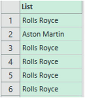
The list resulting from a conversion-to-list operation
This list can now be used in certain circumstances when carrying out more advanced data transformation processes.
Reusing Data Sources
Over the course of Chapters 2 through 5, you saw how to access data from a wide variety of sources to build a series of queries across a range of reports. The reality will probably be that you will frequently want to point to the same sources of data over and over again. In anticipation of this, the Power Query development team has found a way to make your life easier.
- 1.
In the Home ribbon, click the Recent Sources button. A dialog containing the most recently used data sources will appear. You can see this in Figure 9-25.
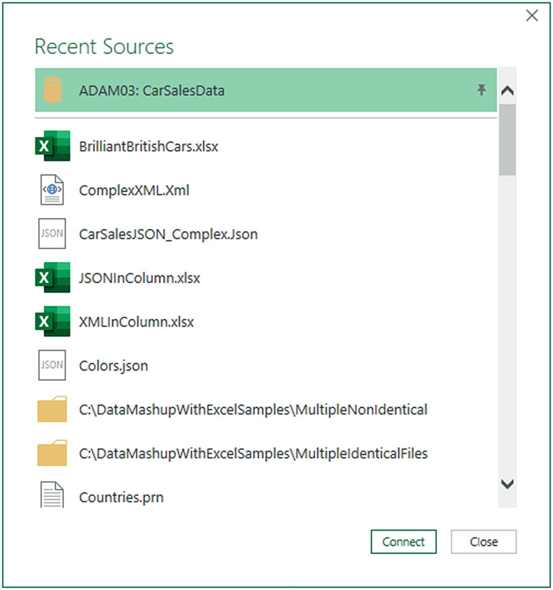
Recently used sources
- 2.
Click the source that you want to reconnect to, and continue with the data load or connection by clicking the Connect button.
Pinning a Data Source
If you look closely at Figure 9-25, you see that the database connection ADAM03:CarSalesData is pinned to the top of the Recent Sources dialog, reflecting a recent database connection that I have made. This allows you to make sure that certain data sources are always kept on hand and ready to reuse.
- 1.
Click the Recent Sources button in the Data ribbon. The Recent Sources dialog will appear.
- 2.
Hover the mouse over a recently used data source. A pin icon will appear at the right of the data source name.
- 3.
Click the pin icon. The data source is pinned to the top of both the Recent Sources menu and the Recent Sources dialog. A small pin icon remains visible at the right of the data source name.
To unpin a data source from the Recent Sources menu and the Recent Sources dialog, all you have to do is click the pin icon for a pinned data source. This unpins it and it reappears in the list of recently used data sources.
Remove from list
Clear unpinned items from list
Copying Data from Power Query Editor
The data in the query
A column of data
A single cell
- 1.Click the element to copy. This can be
- a.
The top-left square of the data grid
- b.
A column title
- c.
A single cell
- a.
- 2.
Right-click and select Copy from the context menu.
You can then paste the data from the clipboard into the destination application.
This process is somewhat limited because you cannot select a range of cells. And you must remember that you are only looking at sample data in the Query Editor. As you can simply load the data into Excel from Power Query, I explain this purely as a minor point that is of limited interest in practice.
Conclusion
This chapter pushed your data transformation knowledge with the Power Query Editor to a new level, by explaining how to deal with multiple file loads of Excel- and text-based data. You then learned ways of handling data from source files that contain complex, nested source structures—specifically JSON and XML files. You also saw how to parse JSON and XML elements from columns contained in other data sources.
Then, you learned how to reuse data sources and manage frequently used data sources to save time. Finally, you learned how to copy sample data resulting from a data transformation process into other applications.
So now the basic tour of data load and transformation with the Power Query Editor is over. It is time to move on to more advanced techniques that you can apply to accelerate and enhance, manage, and structure your data transformation processes and add a certain level of interactivity. These approaches are the subject of the following two chapters.