
In the previous two chapters, you saw how to hone your dataset in Power Query so that you defined only the rows and columns of data that you really need as the basis for your analysis. Then you learned how to cleanse and complete the data that they contain. In this chapter, you will learn how to build on these foundations to deliver data that is ready to be molded into a structured and usable data model.
Joining queries: This involves taking two queries and linking them so that you display the data from both sources as a single dataset. You will learn how to extend a query with multiple columns from a second query as well as how to aggregate the data from a second query and add this to the initial dataset. You will also see how to create complex joins when merging queries.
Pivoting and unpivoting data: If you need to switch data in rows to display as columns—or vice versa—then you can get the Power Query Editor to help you do exactly this. This means that you can guarantee that the data in all the tables that you are using conforms to a standardized tabular structure that is essential for Power Query to function efficiently.
Transposing data: This can be required to switch columns into rows and vice versa.
These techniques can be—and probably will be—used alongside many of the techniques that you saw previously in Chapters 6 and 7. After all, one of the great strengths of Power Query is that it recognizes that data transformation is a complex business and consequently does not impose any strict way of working. Indeed, it lets you experiment freely with a multitude of data transformation options. So remember that you are at liberty to take any approach you want when transforming source data. The only thing that matters is that you use it to give you the result that you want.
The Power Query Editor View Ribbon
The Power Query View ribbon
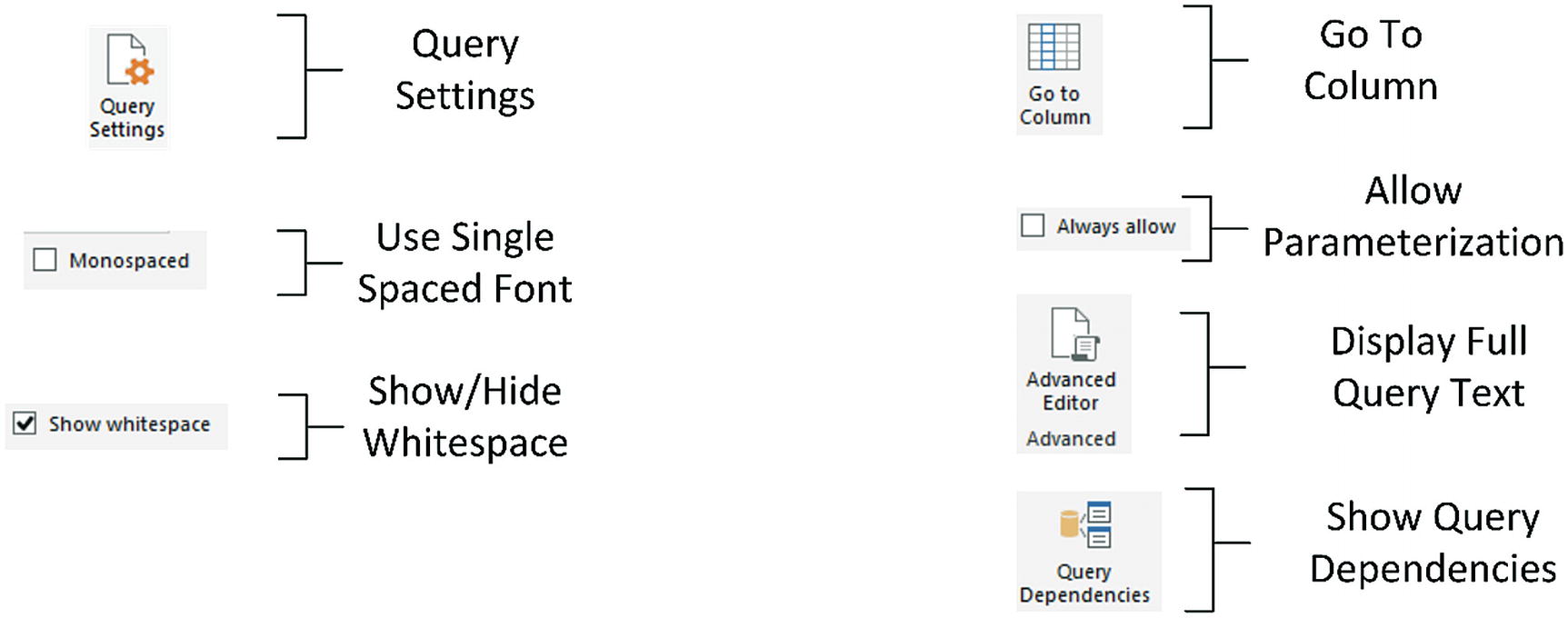
Power Query View Ribbon Options
Option | Description |
|---|---|
Query Settings | Displays or hides the Query Settings pane at the right of the Power Query window. This includes the Applied Steps list |
Monospaced | Displays previews in a monospaced font |
Show whitespace | Displays whitespace and new line characters |
Go to Column | Allows you to select a specific column |
Always allow | Allows parameterization in data source and transformation dialogs. Parameterization is the subject of Chapter 11 |
Advanced Editor | Displays the Advanced Editor dialog containing all the code for the steps in the query |
Query Dependencies | Displays the sequence of query links and dependencies |
Possibly the only option that is not immediately self-explanatory is the Advanced Editor button. It displays the code for all the transformations in the query as a single block of “M” language script. You will learn more about this in Chapter 12.
Personally, I find that the Query Settings pane and the formula bar are too vital to be removed from the Power Query window when transforming data. Consequently, I tend to leave them visible. If you need the screen real estate, however, then you can always hide them for a while.
Merging Data
Look up data elements in another “reference” table to add lookup data. For example, you may want to add a client name where only the client reference code or number exists in your main table.
Aggregate data from a “detail” table (such as invoice lines) and include the totals in a higher-grained table, such as a table of invoices.
Here, again, the process is not difficult. The only fundamental factor is that the two tables, or queries, that you are merging must have a shared field or fields that enable the two tables to match records coherently. Let’s look at a couple of examples.
Extending a Query with Merged Data
- 1.
In a new, empty Excel file, use Power Query to connect to both the worksheets in the C:DataMashupWithExcelSamplesSalesData.xlsx Excel file. These are Sales and Clients.
- 2.
Do not load the data, but click the Transform data button in the Home ribbon. This will display the two separate source datasets in the Power Query Editor.
- 3.
Click the query named Sales in the Queries pane of the Power Query window.
- 4.
Click the Merge Queries button in the Home ribbon. The Merge dialog will appear.
- 5.
In the upper part of the dialog—where an overview of the output from the current query is displayed—scroll to the right and click the ClientName column title. This column is highlighted.
- 6.
In the popup under the upper table, select the Clients query. The output from this query will appear in the lower part of the dialog.
- 7.
In the lower table, select the column title for the column—the join column—that maps to the column that you selected in step 5. This will also be the ClientName column. This column is then selected in the lower table.
- 8.
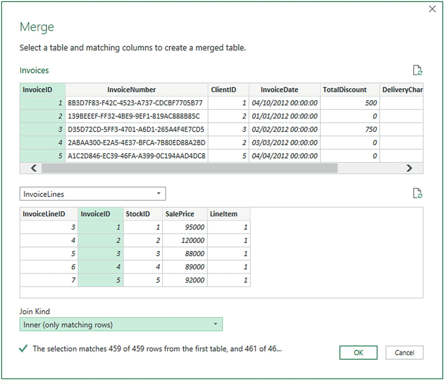
Select Inner (only matching rows) from the Join Kind popup menu. The dialog will look like Figure 8-2.
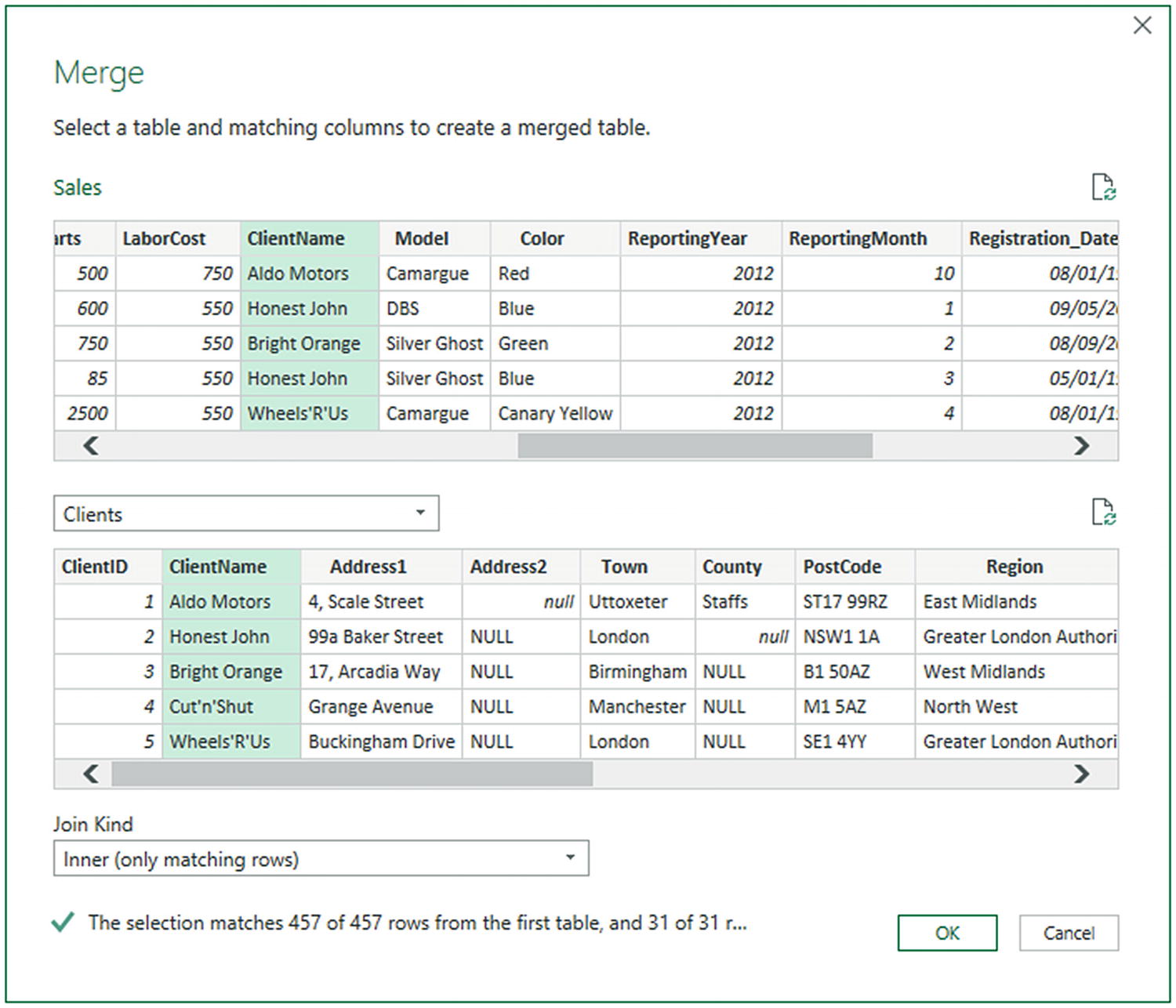
The Merge dialog
- 9.
Click OK. A new column is added to the right of the existing data table. It is named Clients—representing the merged table.
- 10.
Scroll to the right of the existing data table. The new column that has just been created from the merge step contains the word Table in every cell. This column will look something like Figure 8-3.
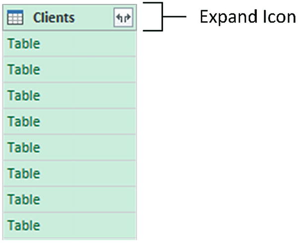
A new, merged column
- 11.
Click the Expand icon to the right of the added column name. The popup list of all the available fields in this data table (or query, if you prefer) is displayed, as shown in Figure 8-4.
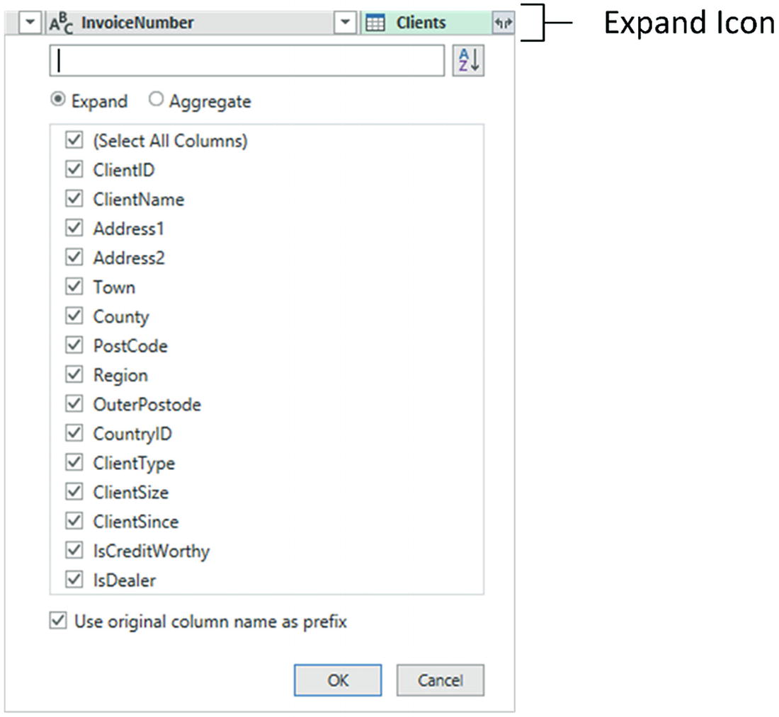
The fields available in a joined query
- 12.
Ensure that the Expand radio button is selected.
- 13.
Clear the selection of all the columns by unchecking the (Select All Columns) check box.
- 14.Select the following columns:
- a.
ClientSize
- b.
ClientSince
- a.
- 15.
Uncheck Use original column name as prefix.
- 16.
Click OK. The selected columns from the merged table are added to the main table, and the link to the reference table (the new column) is removed.
- 17.
Rename the columns that have been added if necessary. The result should look like that in Figure 8-5.

Merged column output
You now have a single table of data that contains data from two linked data sources. Reprocessing the Sales query will also reprocess the dependent clients query and result in the latest version of the data being reloaded.
It is worth noting that it is not necessary to select from the second query any columns that you have already selected from the first query or you will simply return duplicate columns.
You probably noticed that the Merge dialog indicated how many matching records there were in the two queries. This can be a useful indication that you have selected the correct column(s) to join the two queries.
Aggregating Data During a Merge Operation
- 1.
Open a new Excel worksheet.
- 2.
In the Data menu, click Get Data ➤ From File ➤ From Workbook.
- 3.
Find the InvoicesAndInvoiceLines.xlsx Excel source file in the C:DataMashupWithExcelSamples folder.
- 4.
Click the Select multiple items check box.
- 5.
Select the two worksheets it contains (Invoices and InvoiceLines) in the Navigator.
- 6.
Click Transform Data. This will create two queries and open the Power Query Editor.
- 7.
Click the query named Invoices in the Queries pane on the left.
- 8.
In the Home ribbon, click the Merge Queries button. The Merge dialog will open. You will see some of the data from the Invoices dataset in the upper part of the dialog.
- 9.
Click anywhere inside the InvoiceID column. This column is selected.
- 10.
In the popup, select the InvoiceLines query. You will see some of the data from the InvoiceLines dataset in the lower part of the dialog.
- 11.
Click anywhere inside the InvoiceID column for the lower table. This column is selected.
- 12.
Select Inner (only matching rows) from the Join Kind popup menu. The dialog will look like Figure 8-6.
The Merge dialog when aggregating data
- 13.
Click OK. The Merge dialog will close and a new column named InvoiceLines will be added at the right of the Invoices query.
- 14.
Scroll to the right of the existing data table. You will see the new column (named InvoiceLines) that contains the word Table in every cell.
- 15.
Click the Expand icon to the right of the new column title (the two arrows facing left and right). The popup list of all the available fields in the InvoiceLines query is displayed.
- 16.
Select the Aggregate radio button.
- 17.
Select the Sum of SalePrice field and uncheck all the others.
- 18.
Uncheck the “Use original column name as prefix” check box. The dialog will look like Figure 8-7.
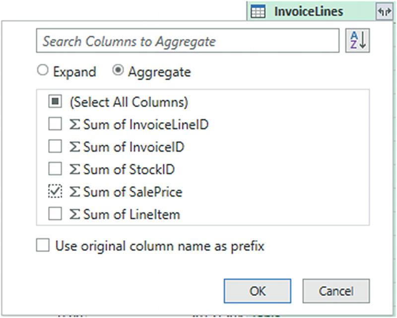
The available fields from a merged dataset
- 19.
Click OK.
Merge Aggregation Options
Option | Description |
|---|---|
Sum | Returns the total value of the field |
Average | Returns the average value of the field |
Median | Returns the median value of the field |
Minimum | Returns the minimum value of the field |
Maximum | Returns the maximum value of the field |
Count (All) | Counts all records in the dataset |
Count (Not Blank) | Counts all records in the dataset that are not empty |
If you loaded the data instead of editing the query in step 1, simply click the Transform Data button in the Home ribbon to switch to the Query Editor.
The merge process that you have just seen, while not complex in itself, suddenly opens up many new horizons. It means that you can now create multiple separate queries that you can then use together to expand your data in ways that allow you to prepare quite complex datasets.
Only queries that have been previously created in the Power Query window can be used when merging datasets. So remember to connect to all the datasets that you require before attempting a merge operation.
Refreshing a query will cause any other queries that are merged into this query to be refreshed also. This way you will always get the most up-to-date data from all the queries in the process.
Merge as a New Query
- 1.
Follow steps 1 through 3 from the section “Extending a Query with Merged Data.”
- 2.
In the Home ribbon, click the small triangle at the right of the Merge Queries button. You can see the available options in the popup menu in Figure 8-8.

Merging tables as a new query
- 3.
Select Merge Queries as New.
- 4.
Continue with steps 5 through 17 from the section “Extending a Query with Merged Data.”
This will create a new query (named Merge—but you can rename it later) and leave the initial queries intact.
This approach can be more fluid and agile than simply extending an existing query. You can rest assured that if you refresh the data, the new merged query will also be refreshed as part of the process.
Types of Join
Join Types
Join Type | Explanation |
|---|---|
Left Outer | Keeps all records in the upper dataset in the Merge dialog (the dataset that was active when you began the merge operation). Any matching rows (those that share common values in the join columns) from the second dataset are kept. All other rows from the second dataset are discarded |
Right Outer | Keeps all records in the lower dataset in the Merge dialog (the dataset that was not active when you began the merge operation). Any matching rows (those that share common values in the join columns) from the upper dataset are kept. All other rows from the upper dataset (the dataset that was active when you began the merge operation) are discarded |
Full Outer | All rows from both queries are retained in the resulting dataset. Any records that do not share common values in the join field(s) contain blanks in certain columns |
Inner | Only joins queries where there is an exact match on the column(s) that are selected for the join. Any rows from either query that do not share common values in the join column(s) are discarded |
Left Anti | Keeps only rows from the upper (first) query |
Right Anti | Keeps only rows from the lower (second) query |
When you use any of the outer joins, you are keeping records that do not have any corresponding records in the second query. Consequently, the resulting dataset contains empty values for some of the columns.
Use original column name as prefix
Search columns to expand
Use the Original Column Name as the Prefix
You will probably find that some columns from joined queries can have the same names in both source datasets. It follows that you need to identify which column came from which dataset. If you leave the check box selected for the “Use original column name as prefix” merge option (which is the default), any merged columns will include the source query name to help you identify the data more accurately.
If you find that these longer column names only get in the way, you can unselect this check box. This will leave the added columns from the second query with their original names. However, because Power Query cannot accept duplicate column names, any new columns will have .1, .2, and so forth added to the column name.
Search Columns to Expand
If you are merging a query with a second query that contains a large number of columns, then it can be laborious to scroll down to locate the columns that you want to include. To narrow your search, you can enter a few characters from the name of the column that you are looking for in the Search columns to aggregate box. The more characters you type, the fewer matching columns are displayed in the Expansion popup dialog.
Joining on Multiple Columns
In the examples so far, you only joined queries on a single column. While this may be possible if you are looking at data that comes from a clearly structured source (such as a relational database), you may need to extend the principle when joining queries from diverse sources. Fortunately, Power Query allows you to join queries on multiple columns when the need arises.
- 1.
In an Excel file, in the Data ribbon, click Get Data ➤ From File ➤ From Workbook and connect to the Excel file C:DataMashupWithExcelSamplesStarSchema.xlsx.
- 2.
Check the Select multiple items check box.
- 3.
Select the two worksheets (Geography and Sales).
- 4.
Click Transform Data to open the Query Editor.
- 5.
Select the Sales query from the list of existing queries from the Queries pane on the left of the Power Query window.
- 6.
In the Home ribbon, click the Merge Queries button. The Merge dialog will appear.
- 7.
In the popup list of queries, select Geography as the second query to join to the first (upper) query.
- 8.
Select Inner (only matching rows) from the Join Kind popup.
- 9.
In the upper list of fields (taken from the Sales table), Ctrl-click the fields CountryName and Region, in this order. A small number will appear to the right of each column header indicating the order that you selected the columns.
- 10.
In the lower list of fields (taken from the Sales table), Ctrl-click the fields CountryName and Region, in this order. A small number will appear to the right of each column header indicating the order that you selected the columns.
- 11.
Verify that you have a reasonable number of matching rows in the information message at the bottom of the dialog. The dialog will look like Figure 8-9.
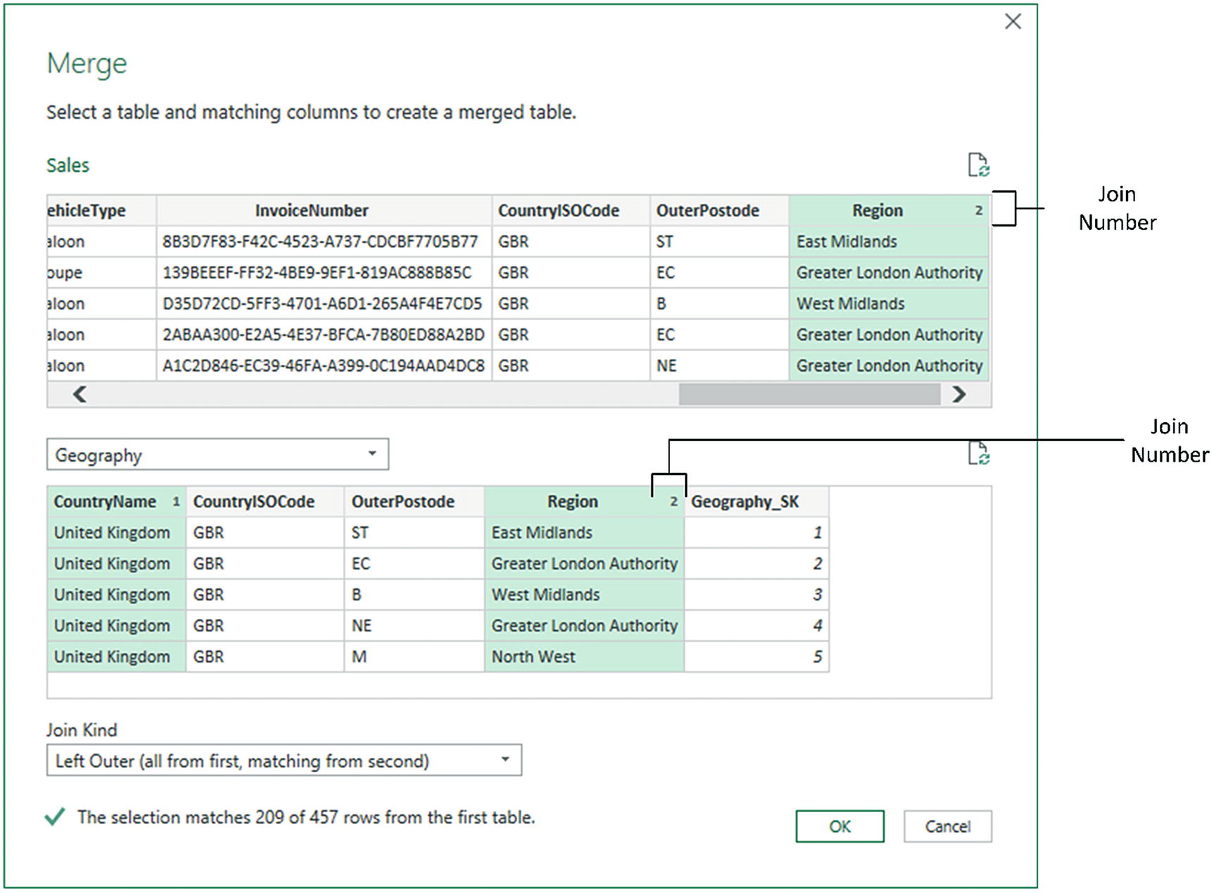
Joining queries using multiple columns
- 12.
Click OK.
You can then continue restructuring your data. In this example, that would be adding the GeographySK field to the Sales query and then removing the Country, Region, and Town fields from the Sales query, for instance.
There is no real limit to the number of columns that can be used when joining queries. It will depend entirely on the shape of the source data. However, each column used to define the join must exist in both datasets, and each pair of columns must be of the same (or a similar) data type.
Preparing Datasets for Joins
You could have to carry out a little preparatory work on real-world datasets before joining queries. More specifically, any columns that you join have to be the same basic data type. Put simply, you need to join text-based columns to other text-based columns, number columns to number columns, and date columns to date columns. If the columns are not the same data type, you receive a warning message when you try to join the columns in the Merge dialog.
Consequently, it is nearly always a good idea to take a look at the columns that you will use to join queries before you start the merge operation itself. Remember that data types do not have to be identical, just similar. So a decimal number type can map to a whole number, for instance.
Removing trailing or leading spaces in text-based columns
Isolating part of a column (either in the original column or as a new column) to use in a join
Verifying that appropriate data types are used in join columns
Correct and Incorrect Joins
The columns do not map.
The columns map, but the result is a massive table with duplicate records.
Let’s take a look at these possible problems.
The Columns Do Not Map
Are the values in the two queries the same data type?
Do the values really map—or are they different?
Are you using the correct columns?
Are you using too many columns and so specifying data that is not in both queries?
The Columns Map, but the Result Is a Massive Table with Duplicate Records
Joining queries depends on isolating unique data in both source queries. Sometimes a single column does not contain enough information to establish a unique reference that can uniquely identify a row in the query.
In these cases, you need to use two or more columns to join queries—or else rows will be duplicated in the result. Therefore, once again, you need to look carefully at the data and decide on the minimum number of columns that you can use to join queries correctly.
A comment at the bottom of the Merge dialog tells you how many records match between the two tables. This can be a valid and useful indicator of whether you have selected the correct join columns and an appropriate join type.
Examining Joined Data
Joining data tables is not always easy. Neither is deciding if the outcome of a merge operation will produce the result that you expect. So Power Query includes a solution to these kinds of dilemma. It can help you more clearly see what a join has done. More specifically, it can show you for each record in the first query exactly which rows are joined from the second query.
- 1.
Carry out steps 1 through 10 in the example you saw earlier (section “Joining on Multiple Columns”).
- 2.
Scroll to the right in the data table. You will see the new column named Geography (as shown in Figure 8-10).
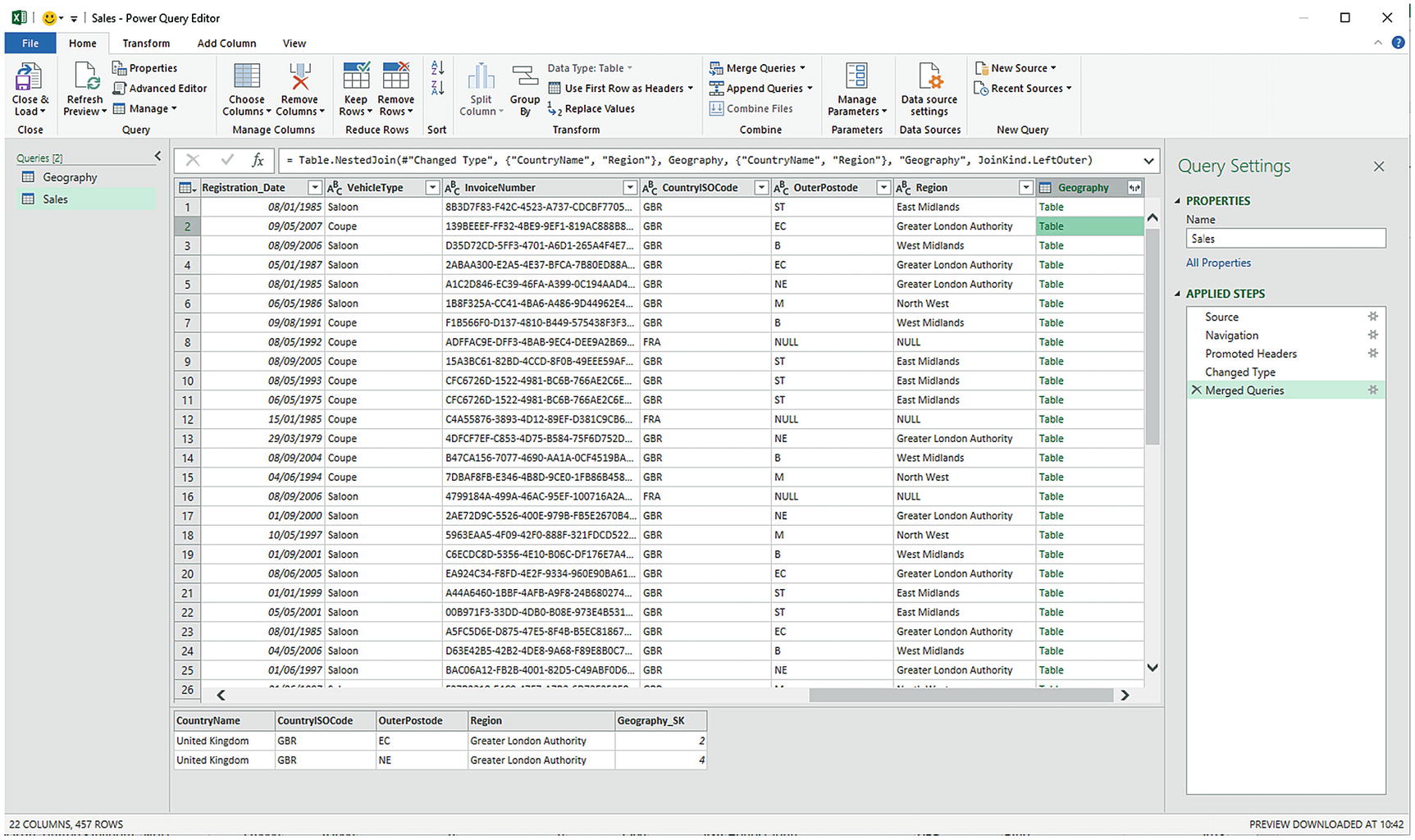
Joined data
- 3.
Click to the right of the word Table in the row where you want to see the joined data. Note that you must not click the word Table. A second table will appear under the main query’s data table containing the data from the second query that is joined for this particular row. Figure 8-10 shows an example of this.
You can resize the lower table (and consequently display more or less data from the second joined table) by dragging the bottom border of the top data table up or down.
Clicking to the right of the word Table in the NewColumn column will enable the Expand and Aggregate buttons in the Transform ribbon.
Clicking the word Table in the NewColumn column adds a new step to the query that replaces the source data with the linked data. You can also do this by right-clicking inside the NewColumn column and selecting Drill Down.
Drilling down into the merged table in effect limits the query to the row(s) of the subtable. Consequently, you have to delete this step if you want to access all the data in the merged tables.
Appending Data
Not all source data is delivered in its entirety in a single file or as a single database table. You may be given access to two or more tables or files that have to be loaded into a single table in Excel or Power Pivot. In some cases, you might find yourself faced with hundreds of files—all text, CSV, or Excel format—and the requirement to load them all into a single table that you will use as a basis for your analysis. Well, Power Query can handle these eventualities, too.
Adding the Contents of One Query to Another
They have the same number of columns.
The columns are in the same order.
The data types are identical for each column.
The columns have the same names.
- 1.Create queries to load each of the following text files into Excel worksheets. As this was explained in Chapter 2, I will not repeat the principles here. Both files are in the C:DataMashupWithExcelSamplesMultipleIdenticalFiles folder:
- a.
Colours_01.txt
- b.
Colours_02.txt
- a.
- 2.
Name the queries Colours_01 and Colours_02. You can see the contents of these two queries in Figure 8-11.
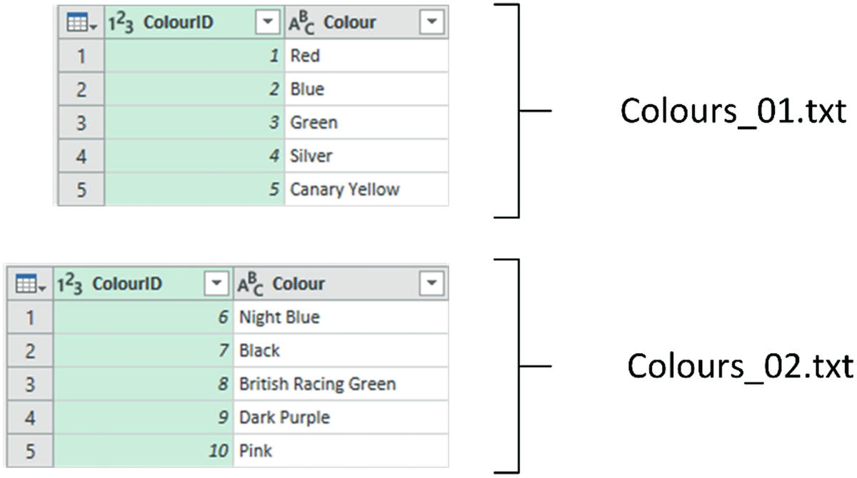
Source data for appending
- 3.
Open one of the queries (I use Colours_01, but either will do) by double-clicking one of the query names in the Queries & Connections pane. This will open the Power Query Editor.
- 4.
Click the arrow to the right of the Append Queries button in the Power Query Editor Home ribbon and select Append queries as new. The Append dialog will appear.
- 5.
Ensure that the Two tables radio button is selected.
- 6.
From the Select Table to Append popup, choose the query Colours_02. The dialog will look like the one in Figure 8-12.
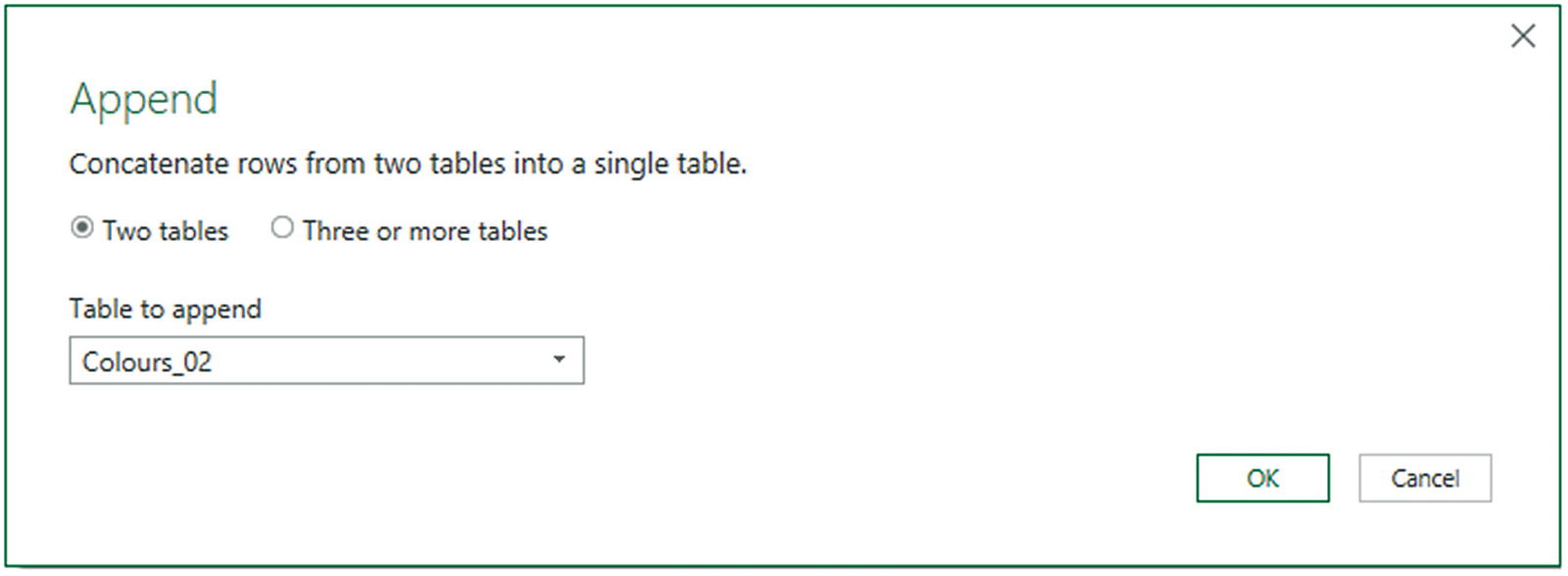
The Append dialog
- 7.
Click OK. The data from the two output tables is appended in a new query. You can see an example of the resulting output in Figure 8-13.
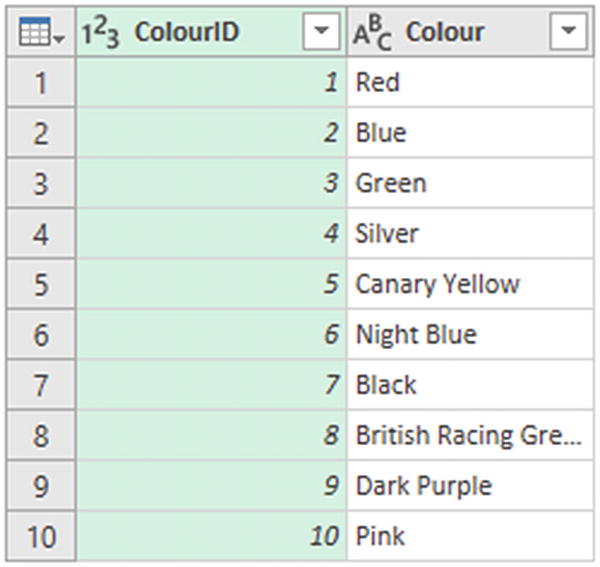
A new query containing appended data
You can now continue with any modifications that you need to apply. You will notice that the column names are not repeated as part of the data when the tables are appended one to the other.
One interesting aspect of this approach is that you have created a link between the two source tables and the new query. This means that when you refresh the source data, not only are the data in the tables Colours_01 and Colours_02 updated but the “derived” query that you just created is updated as well.
Appending the Contents of Multiple Queries
The Query Editor does not limit you to appending only two files at once. You can (if you really need to) append a virtually limitless number of identical files.
- 1.
Create queries to load the data in the worksheet named BaseData in the Excel file BrilliantBritishCars1.xlsx in the folder C:DataMashupWithExcelSamplesMultipleIdenticalExcel.
- 2.
Repeat step 1 to load the data contained in the files BrilliantBritishCars2.xlsx and BrilliantBritishCars3.xlsx that are also in the folder C:DataMashupWithExcelSamplesMultipleIdenticalExcel.
- 3.
Double-click the query named BaseData in the Queries & Connections pane on the right to open the Query Editor.
- 4.
Click the Append Queries button.
- 5.
Select the Three or more tables radio button in the Append dialog.
- 6.
Ctrl-click the tables “BaseData (2)” and “BaseData (3)” in the Available table(s) list on the left of the dialog.
- 7.
Click the Add button. You can see what the Append dialog now looks like in Figure 8-14.
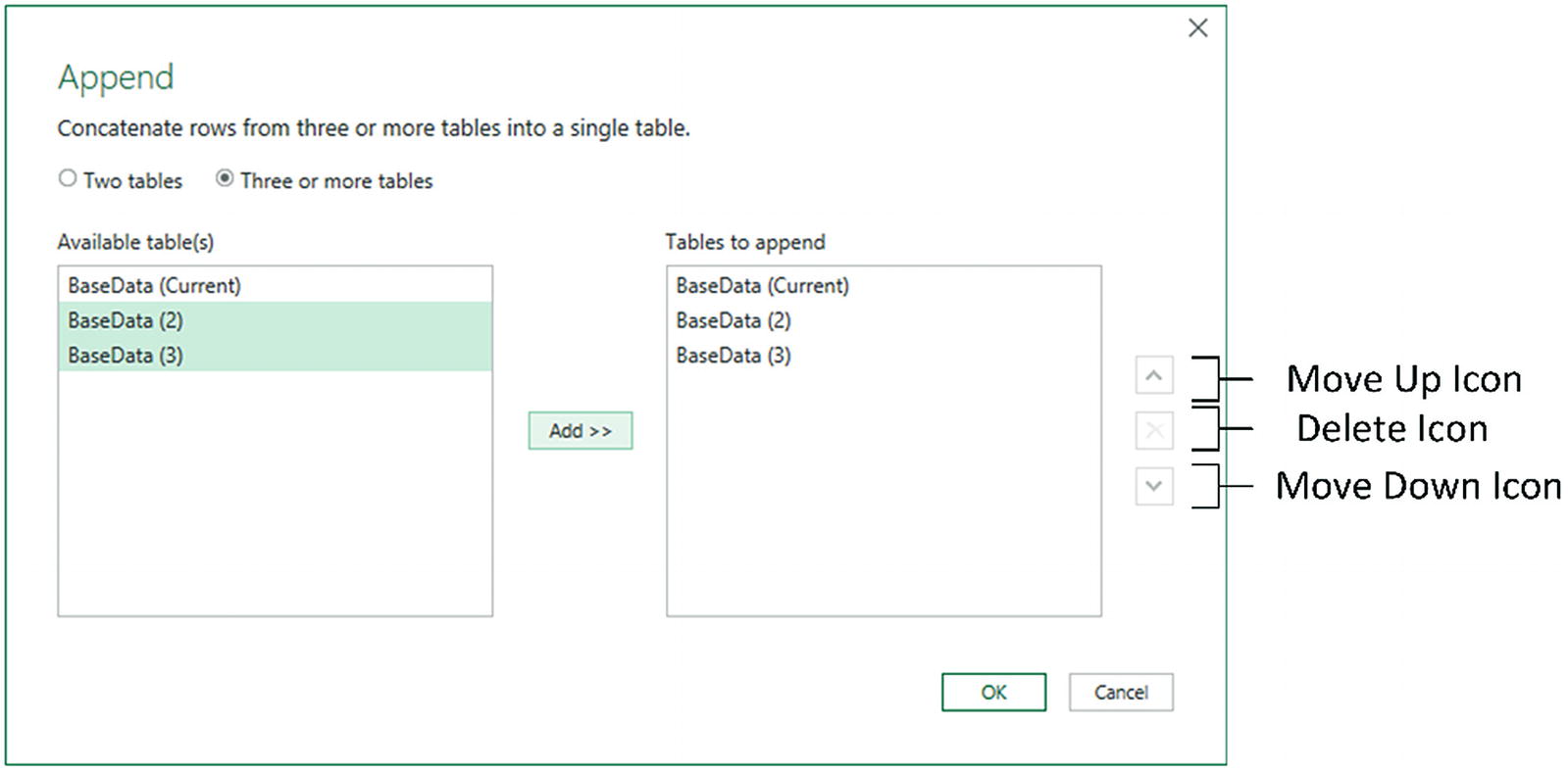
Appending multiple queries
- 8.
Click OK. The data from the query “BaseData (2)” and “BaseData (3)” will be appended to the current query (BaseData).
Remove queries from the list of queries to append on the right by clicking the query (or Ctrl-clicking multiple queries) and subsequently clicking the cross icon on the right of the dialog.
You can alter the load order of queries by clicking the query to move and then clicking the up and down chevrons on the right of the dialog.
Changing the Data Structure
Unpivoting data
Pivoting data
Transforming rows and columns
Each of these techniques is designed to meet a specific, yet frequent, need in data loading, and all are described in the next few pages.
Unpivoting Tables
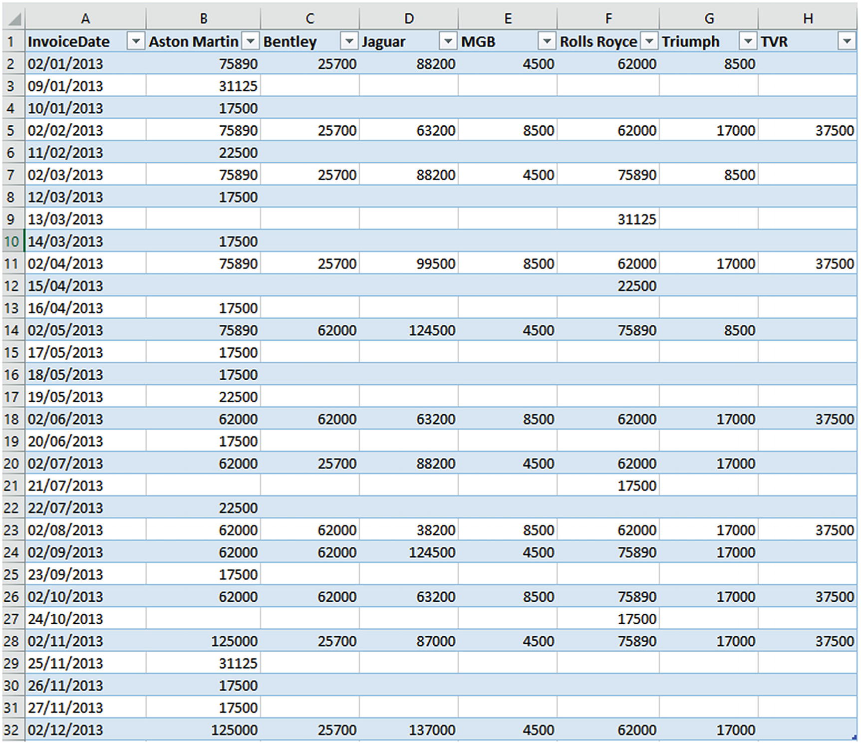
A pivoted dataset
- 1.
In a new Excel file, click Get Data ➤ From File ➤ From Excel to connect to the table PivotedCosts from the C:DataMashupWithExcelSamplesPivotedDataSet.xlsx file into Power Query. Be sure not to load the data, but to click Transform Data from the Navigator.
- 2.
Ensure that the first row is set to be the table headers.
- 3.
In the Query Editor, select all the columns that you want to unpivot. In this example, this means all columns except the first one (all the makes of cars).
- 4.
In the Transform ribbon, click the Unpivot Columns button (or right-click any of the selected columns and choose Unpivot Columns from the context menu). The table is reorganized and the first few records look as they do in Figure 8-16. Unpivoted Columns is added to the Applied Steps list.
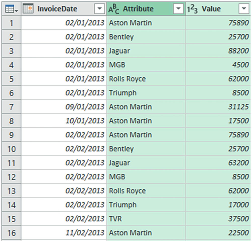
An unpivoted dataset
- 5.
Rename the columns that Power Query has named Attribute and Value.
The data is now presented in a standard tabular way, and so it can be used to create a data model (or loaded into an Excel worksheet) to serve as the basis for further analysis.
The Unpivot button contains another menu option that is displayed if you click the small triangle to the right of the Unpivot button. This is the Unpivot Other Columns option that will switch the contents of columns into rows for all the columns that are not selected when you run the transformation.
Unpivot Options
Unpivot Other Columns: This will add the contents of all the other columns to the unpivoted output.
Unpivot Only Selected Columns: This will only add the contents of any preselected columns to the unpivoted output.
As is the case with so many of the techniques that you apply using the Query Editor, it is really important to select the appropriate column(s) before carrying out pivot and unpivot operations.
Pivoting Tables
- 1.
Follow steps 1 through 3 of the previous section so that you end up with the table of data that you can see in Figure 8-15.
- 2.
Click inside the column Attribute.
- 3.
In the Transform ribbon, click the Pivot Column button. The Pivot Column dialog will appear.
- 4.
Select Value (the column of figures) as the values column that is aggregated by the pivot transformation.
- 5.
Expand Advanced options and ensure that Sum is selected as the Aggregate Value Function. The Pivot Column dialog will look like Figure 8-17.
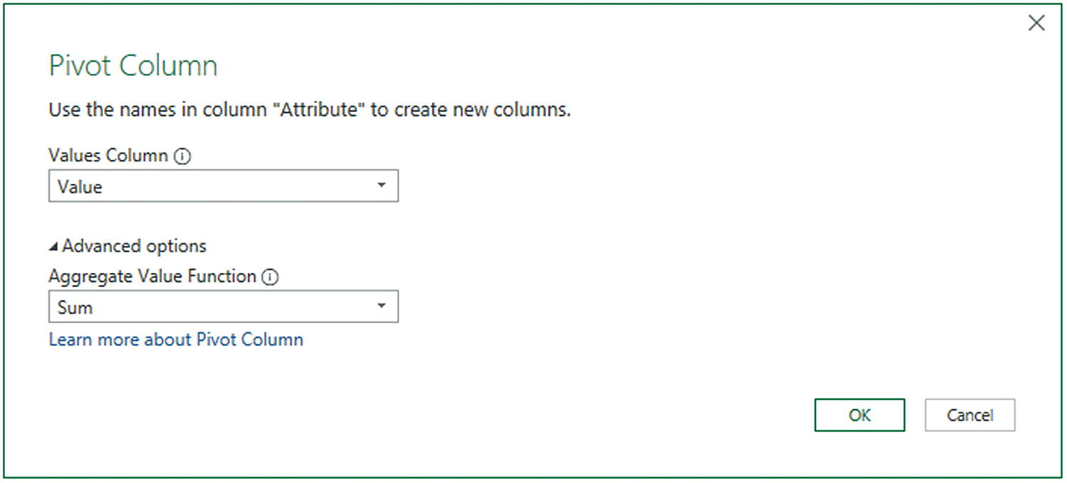
The Pivot Column dialog
- 6.
Click OK. The table is pivoted and looks like Figure 8-18. Pivoted Column is added to the Applied Steps list.
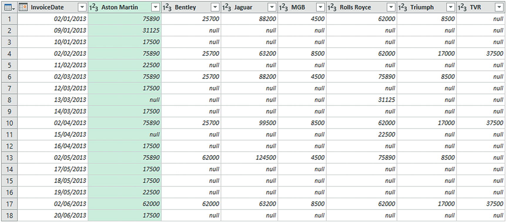
Pivoted data
The Advanced options section of the Pivot Column dialog lets you choose the aggregation operation that is applied to the values in the pivoted table.
Transposing Rows and Columns
- 1.
Connect to the Excel file C:DataMashupWithExcelSamplesDataToTranspose.xlsx in the Power Query Editor. You will need to select Sheet1. You will see a data table like the one in Figure 8-19.

A dataset needing to be transposed
- 2.
In the Transform ribbon, click the Transpose button. The data is transposed and appears as two columns, just like the CountryList.txt file that you saw in Chapter 2.
- 3.
Rename the resulting columns.
Loading Data from Inside the Query Editor Directly
- 1.
In the Query Editor, expand the Queries pane on the left (unless it is already displayed).
- 2.
Right-click inside Queries pane.
- 3.
Select New Query ➤ File ➤ Text/CSV. You can see this popup menu in Figure 8-20.
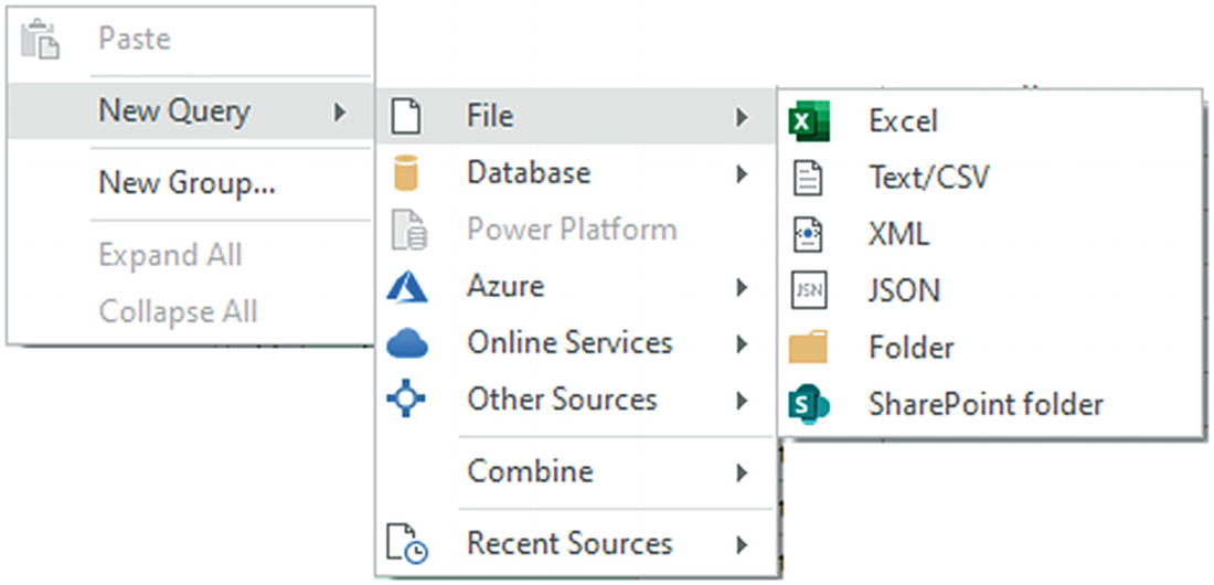
The popup menu to add further queries directly inside the Power Query Editor
- 4.
Load the CSV file Countries.csv, as you learned in Chapter 2.
A new query will be added to the Queries pane in the Power Query Editor as well as in the Connections & Queries pane in Excel.
This technique, although somewhat hidden, can be particularly useful as it avoids you having to close the Query Editor to create a new query—only to return to the Query Editor to continue working. All the data source options that were available in the Excel Get Data button are present when creating new queries inside the Query Editor.
As you are already inside the Query Editor, there is no Transform Data button when connecting to a new data source. You are, to all intents and purposes, already transforming the data.
Error Display
Sometimes source data may be clearly erroneous. In these cases, Power Query will flag cells that contain obvious errors. It does not presume to modify the data—after all, the data might be useful even if it is flagged as containing errors or anomalies.
- 1.
Open a new, blank Excel workbook.
- 2.
Click Data ➤ Get Data ➤ From File ➤ From Workbook.
- 3.
Select the Excel file SampleErrors.xlsx and click Import.
- 4.
Select Sheet1 and click Transform Data to display the data in the Power Query Editor.
- 5.
Click inside the column Price and, in the Home ribbon, set the data type to decimal number.
- 6.
Click Replace current in the Change Column Type dialog that appears. Two of the rows will display errors, as shown in Figure 8-21.
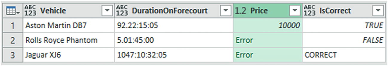
Displaying errors
In some datasets, the data that is flagged as being an error could be the data that you want to examine in greater detail. The point is that you can see potential errors and decide whether to remove them (as described later) or to return to the source data and correct them before reloading the data.
Removing Errors
- 1.
Click inside the column containing errors; or if you want to remove errors from several columns at once, Ctrl-click the titles of the columns that contain the errors.
- 2.
Click the popup triangle in the Remove Rows button in the Home ribbon. The popup menu will appear.
- 3.
Click Remove errors. Any records with errors flagged in the selected columns are deleted. Removed Errors is added to the Applied Steps list.
You have to be very careful here not to remove valid data. Only you can judge, once you have taken a look at the data, if an error in a column means that the data can be discarded safely. In all other cases, you would be best advised to look at cleansing the data or simply leaving records that contain errors in place. The range and variety of potential errors are as vast as the data itself.
Viewing Errors
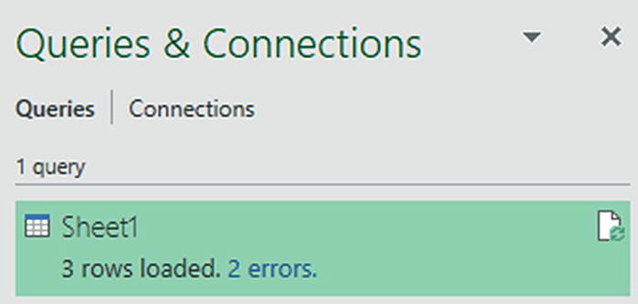
Displaying queries with errors in the Queries & Connections pane
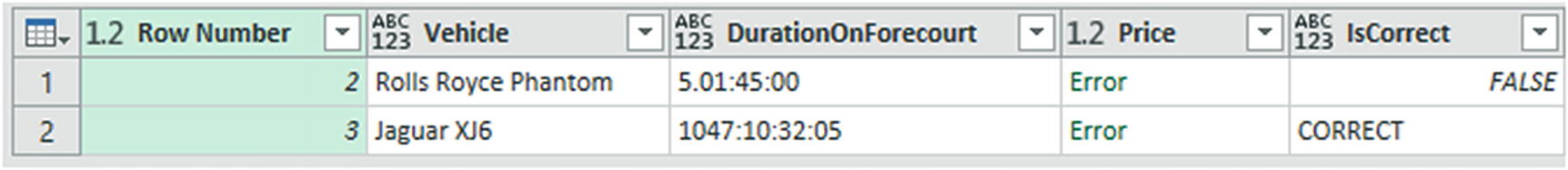
Displaying error records only
Data Transformation Approaches
If in doubt, right-click the column that you want to transform. This will list the most common available options in the context menu.
To alter existing data, use the Transform menu.
To add a new column, use the New Column menu.
Remember that you can “unwind” your modifications by deleting steps in the data transformation process.
Conclusion
This chapter showed you how to structure your source data into a valid data table from one or more potential sources. Among other things, you saw how to pivot and unpivot data, to fill rows up and down with data, as well as how to transpose rows and columns.
Possibly the most important thing that you have learned is how to join individual queries so that you can add the data from one query into another. This can involve looking up data from a separate query or carrying the aggregated results from one query into another.
Finally, you learned how to identify error records in a query.
Now it is time to push your data transformation skills to the next level and learn how to set up complex data ingestion and conversion routines. These are the subject of Chapter 9.