
| Name | Layers | Top-5 Error (%) | References |
| AlexNet | 8 | 15.3 | Krizhevsky et al. (2012) |
| VGG Net | 19 | 7.3 | Simonyan and Zisserman (2014) |
| ResNet | 152 | 3.6 | He et al. (2016) |

From Image Filtering to Learnable Convolutional Layers
When an image is filtered, the output is another image that contains the filter’s response at each spatial location, e.g., one with its edges emphasized. We could also think of such an image as a feature map that indicates where certain features were detected in the image—e.g., edges. However, in a deep network the initial filtered images or feature maps are subjected to many further levels of filtering. Over many successive filter applications this produces spatially organized neurons that respond to much more complex inputs, and the term “feature map” becomes more descriptive.
When viewed as layers in a neural network that takes an image as input, these filtering operations can be viewed as constraining spatially organized neurons to respond only to features that are within a limited region of the input known as the neuron’s receptive field. When groups of such neurons respond in the same way to the same types of input we say they have shared parameters—but each neuron forming the feature map responds only when certain inputs are detected at corresponding spatially restricted receptive fields in the image.
Consider a simple example with a 1D vector x. A filtering operation can be implemented by multiplying it by a matrix W that has a special structure, such as

where the blank elements are zero. This matrix corresponds to a simple filter having only three nonzero coefficients and a “stride” of one. To account for samples at the beginning and end of the input, or pixels at the edge of the image in the 2D case, zeros can be placed before the start and end, or around the image boundary—e.g., a zero could be added to the start and end of x above, in which case the output would have the same size as the input. If we dispensed with zero-padding, the valid part of the convolution would be restricted to filter responses computed from input data.
If the rows of a 2D image were packed into one long column vector, a version of this same 3×3 filter could be achieved by a much larger matrix W, having two other sets of three coefficients further along each row. The result would implement the multiplication and additions performed by the matrix encoding of a 2D filter. This could be thought of in another way, as an operation known in signal processing as the cross-correlation or sliding dot product, which is closely related to a computation known as convolution.
Suppose the filter above is centered by giving the first vector element an index of −1, or, in general, an index of −K, where K is the “radius” of the filter. The 1D filtering is then
Directly generalizing this filtering to a 2D image X and filter W gives the cross-correlation, Y=W![]() X, for which the result for row r and column c is
X, for which the result for row r and column c is
The convolution of an image with a filter, ![]() , is obtained by flipping the sense of the filter,
, is obtained by flipping the sense of the filter,
As an example, consider the task of detecting edges in an image. A well-known technique is to filter it with so-called “Sobel” filters, which involve cross-correlating or convolving it with:

These particular filters behave much like derivatives of the image. Fig. 10.8 shows the result: a photograph; a version filtered with the Sobel operator Gx, which emphasizes vertical edges; a version filtered with the Sobel operator Gy, which emphasizes horizontal edges; and the result of computing ![]() . The center two images have been scaled so that midgray corresponds to zero, while the intensity is flipped in the last one to make large values darker and white zero.
. The center two images have been scaled so that midgray corresponds to zero, while the intensity is flipped in the last one to make large values darker and white zero.
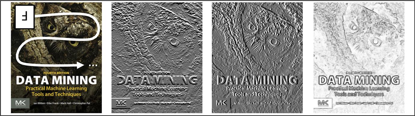
Rather than using predetermined filters, convolutional networks jointly learn sets of convolutional filters and a classifier that takes them as input, everything being learned together by backpropagation. By convolving the image with filters successively within the layers of a neural network spatially organized hidden layers can be created, which, as discussed above, could be thought of as feature activity maps indicating where a given feature type has been detected within the image. While filters and activation functions are not specifically constructed as shown in Fig. 10.8, edge-like filters and texture-like filters are frequently observed in the early layers of CNNs that have been trained using natural images. Since each layer in a CNN involves filtering the feature map produced by the layer below, as one moves upwards the receptive field of any given neuron or feature detector becomes larger. As a result, after learning, higher-level layers detect larger features, which often correspond to small pieces of objects in midlevel layers, and quite large pieces of objects toward the top of the network. Fig. 10.9 shows examples of the strongest activation of some random neurons in each layer, projecting the activation back into image space using deconvolution.

Spatial pooling operations applied to the result of a convolutional network are frequently used to impart a degree of local spatial invariance to the precise locations where features have been detected. If pooling is done by averaging, it can be implemented using convolutions. CNNs often apply multiple layers of convolution, followed by pooling and decimation layers. It is common to have about three phases of pooling and decimation. After the last pooling and decimation layer the resulting feature maps are typically fed into a multilayer perceptron. Since decimation reduces the size of feature maps, each such operation reduces the size of subsequent activity maps. Extremely deep convolutional network architectures (having more than 8 layers) typically repeat convolutional layers many times before applying the pooling and decimation operations.
Fig. 10.10 shows a numerical example of the key operations of convolution, pooling, and decimation. First, an image is convolved with the (flipped) filter shown on the left. The curved rectangular regions in the image matrix depict a random set of image locations. The next matrix shows the result of the convolution operation, and here the maximum values within small 2×2 regions are indicated in bold. Next the result is pooled, using max-pooling in this case; and then the pooled matrix is decimated by a factor of two to yield the final result.

Convolutional Layers and Gradients
Let us consider how to compute the gradients needed to optimize a convolutional network. At a given layer we have i=1,…, N(l) feature filters and corresponding feature maps. The convolutional kernel matrices Ki contain flipped weights with respect to kernel weight matrices Wi. With activation function act(), and for each feature type i a scaling factor gi and bias matrix Bi, the feature maps are matrices Hi(Ai(X)) and can be visualized as a set of feature map images given by
The loss ![]() is a function of the N(l) feature maps for a given layer. Define h=vec(H), x=vec(X), a=vec(A), where the vec() function returns a vector with stacked columns of the given matrix argument. Choose an act() function that operates elementwise on an input matrix of preactivations and has scale parameters of 1 and biases of 0. The partial derivatives of the hidden layer output with respect to X of the convolutional units are
is a function of the N(l) feature maps for a given layer. Define h=vec(H), x=vec(X), a=vec(A), where the vec() function returns a vector with stacked columns of the given matrix argument. Choose an act() function that operates elementwise on an input matrix of preactivations and has scale parameters of 1 and biases of 0. The partial derivatives of the hidden layer output with respect to X of the convolutional units are
where ![]() is a matrix containing the partial derivative of the elementwise act() function’s input with respect to its preactivation value for the ith feature type, organized according to spatial positions given by row j and column k. Intuitively, the result is a sum of the convolution of each of the (zero padded) filters Wi with an image-like matrix of derivatives Di. The partial derivatives of the hidden layer output are
is a matrix containing the partial derivative of the elementwise act() function’s input with respect to its preactivation value for the ith feature type, organized according to spatial positions given by row j and column k. Intuitively, the result is a sum of the convolution of each of the (zero padded) filters Wi with an image-like matrix of derivatives Di. The partial derivatives of the hidden layer output are
where ![]() is the row- and column-flipped version of the input X (if the convolution is written as a linear matrix operation, this will involve just a matrix transpose).
is the row- and column-flipped version of the input X (if the convolution is written as a linear matrix operation, this will involve just a matrix transpose).
Pooling and Subsampling Layers and Gradients
Consider applying a pooling operation to a spatially organized feature map. The input consists of matrices Hi for each feature map, with elements hijk. The max pooled and average pooled feature maps are matrices Pi with elements pijk given by

respectively, where Rj,k and Cj,k are sets of indices that encode the pooling regions for each location j, k, and m is the number of elements in the pooling region. Although these pooling operations do not include a subsampling step, they typically account for boundary effects either by creating a matrix Pi that is slightly smaller than the input matrix Hi, or by padding with zeros. The subsampling step either samples every nth output, or avoids needless computation by only evaluating every nth pooling computation.
What are the consequences of backpropagating gradients through layers consisting of max or average pooling? In the former case, the units that are responsible for the maximum within each zone j, k —the “winning units”—are given by
For nonoverlapping zones, the gradient is propagated back from the pooled layer Pi to the original spatial feature layer Hi, flowing from each pijk to just the winning unit in each zone. This can be written

In the latter case, average pooling, the averaging operation is simply a special type of convolution with a fixed kernel that computes the (possibly weighted) average of pixels in a zone, so the required gradients are computed using the result above. These various pieces are the building blocks that allow for the implementation of a CNN according to a given architecture.
Implementation
Convolutions are particularly well suited to implementation on graphics hardware. Since graphics hardware can accelerate convolutions by an order of magnitude or more over CPU implementations, it plays an important role in training CNNs. An experimental turn-around time of days rather than weeks makes a huge difference to model development times.
It can also be challenging to construct software for learning a CNN in such a way that alternative architectures can be explored. Although early GPU implementations were hard to extend, newer tools allow for both fast computation and flexible high-level programming primitives. Some of these tools are discussed at the end of this chapter; many of them allow gradient computations and the backpropagation algorithm for large networks to be almost completely automated.
10.4 Autoencoders
Neural networks can also be used for unsupervised learning. An “autoencoder” is a network that learns an efficient coding of its input. The objective is simply to reconstruct the input, but through the intermediary of a compressed or reduced-dimensional representation. If the output is formulated using probability, the objective function is to optimize ![]() , i.e., the probability that the model gives a random variable
, i.e., the probability that the model gives a random variable ![]() the value
the value ![]() given the observation
given the observation ![]() , where
, where ![]() . In other words, the model is trained to predict its own input—but it must map it through a representation created by the hidden units of a network.
. In other words, the model is trained to predict its own input—but it must map it through a representation created by the hidden units of a network.
Fig. 10.11 shows a simple autoencoder, where ![]() . The parameters of the final probabilistic prediction are given by the last layer’s activation function
. The parameters of the final probabilistic prediction are given by the last layer’s activation function ![]() , which is created using a neural network consisting of an encoding step
, which is created using a neural network consisting of an encoding step ![]() followed by a decoding step
followed by a decoding step ![]() , using the same matrix W in both steps. Each function has its own bias vector b(i). Since the idea of an autoencoder is to compress the data into a lower-dimensional representation, the number L of hidden units used for encoding is less than the number M in the input and output layers. Optimizing the autoencoder using the negative log probability over a data set as the objective function leads to the usual forms. Like other neural networks it is typical to optimize autoencoders using backpropagation with mini-batch based stochastic gradient descent.
, using the same matrix W in both steps. Each function has its own bias vector b(i). Since the idea of an autoencoder is to compress the data into a lower-dimensional representation, the number L of hidden units used for encoding is less than the number M in the input and output layers. Optimizing the autoencoder using the negative log probability over a data set as the objective function leads to the usual forms. Like other neural networks it is typical to optimize autoencoders using backpropagation with mini-batch based stochastic gradient descent.

Both the encoder activation function act() and the output activation function out() in Fig. 10.11 could be defined as the sigmoid function. It can be shown that with no activation function, h(i)=a(i), the resulting “linear autoencoder” will find the same subspace as principal component analysis, assuming a squared-error loss function and normalizing the data using mean centering. This autoencoder can be shown to be optimal in the sense that any model with a nonlinear activation function would require a weight matrix with more parameters to achieve the same reconstruction error. It is known that even with a nonlinear activation function such as the sigmoid function, optimization will tend toward solutions where the network operates in the linear regime of the sigmoid, replicating the behavior of principal component analysis.
This might seem discouraging: linear autoencoders are no better than principal component analysis. However, using a neural network with even one hidden layer to create an encoding can construct much more flexible transformations, and there is growing evidence that deeper models can learn more useful representations. When building autoencoders from more flexible models, it is common to use a bottleneck in the network to produce an under-complete representation, providing a mechanism to obtain an encoding of lower dimension than the input.
Deep autoencoders are able to learn low-dimensional representations with smaller reconstruction error than principal component analysis using the same number of dimensions. They are constructed by using L layers to create a hidden layer representation ![]() of the data, and following this with a further L layers
of the data, and following this with a further L layers ![]() to decode the representation back into its original form, as shown in Fig. 10.12. The j=1,…, 2L weight matrices for each of the i=1,…, L encoding and decoding layers are constrained by
to decode the representation back into its original form, as shown in Fig. 10.12. The j=1,…, 2L weight matrices for each of the i=1,…, L encoding and decoding layers are constrained by ![]() .
.

A deep encoder for ![]() has the form
has the form
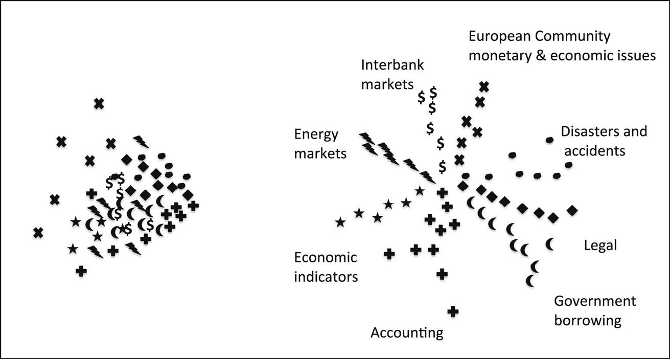
Fig. 10.13 compares data projected into a 2D space learned in this way with 2D principal component analysis for a particular data set. Since the underlying autoencoder is nonlinear, the network can arrange the learned space in such a way that it better separates natural groupings of the data.
Pretraining Deep Autoencoders With Rbms
Deep autoencoders are an effective framework for nonlinear dimensionality reduction. Once such a network has been built, the top-most layer of the encoder, the code layer hc, can be input to a supervised classification procedure. If a neural network classifier is used, the entire deep autoencoder network can be discriminatively fine-tuned using gradient descent. In effect, the autoencoder approach is used to pretrain a neural network classifier.
However, it is difficult to optimize autoencoders with multiple hidden layers in both encoder and decoder. It is well known that initializing any deep neural network with weights that are too large leads to poor local minima; while initialization with weights that are too small can lead to small gradients that make learning slow. One approach is to be very careful about the choices of activation function and initialization. However, this has been found difficult in practice.
Another approach is based on pretraining by stacking two-layered RBMs. RBMs are a generalized form of probabilistic PCA with binary hidden variables and binary or continuous observed variables that can perform unsupervised learning; they are discussed further in Section 10.5; To use them for pretraining, start by learning a 2-layer RBM from the data, project the data into its hidden-layer representation, use that to train another RBM, and repeat the process until the encoding layer is reached. The details of how this is done is described in Section 10.5. The parameters of each two-layer network are then used to initialize the parameters of an autoencoder with a similar structure that has nonstochastic sigmoid hidden units.
Denoising Autoencoders and Layerwise Training
One can also use greedy layerwise training strategies involving plain autoencoders to train deep autoencoders, but attempts to do this for networks of even moderate depth have encountered difficulties. Procedures based on stacking denoising autoencoders have been found to work better. Denoising autoencoders are trained to remove different types of noise that has been added synthetically to their inputs. Autoencoder inputs can be corrupted with noise such as: Gaussian noise; masking noise, where some elements are set to 0; and salt-and-pepper noise, where some elements are set to minimum and maximum input values (such as 0 and 1).
Using autoencoders with stochastic hidden units involves fairly minor modifications to backpropagation based learning. In essence, these procedures resemble dropout. In contrast, more general stochastic models like RBMs rely on approximate probabilistic inference techniques, and the procedures for learning deep stochastic models tend to be quite elaborate (see Section 10.5).
Combining Reconstructive and Discriminative Learning
When an autoencoder is used to learn a feature representation intended for classification or regression, a model can be defined that both reconstructs inputs and classifies inputs. This hybrid model has a composite loss that consists of a reconstructive (unsupervised) and a discriminative (supervised) criterion, ![]() , where the hyperparameter
, where the hyperparameter ![]() controls the balance between the two objectives. In the extreme cases,
controls the balance between the two objectives. In the extreme cases, ![]() yields a purely supervised training procedure, while
yields a purely supervised training procedure, while ![]() yields a purely unsupervised training procedure. If some data is only available without labels, one can optimize just a reconstructive loss. For the hybrid model, one could imagine augmenting the deep autoencoder of Fig. 10.12 to make predictions using hc as input, either with a single set of weights leading to an activation function and final prediction, or with multiple layers prior to making a prediction. Training with a combined objective function appears to provide a form of regularization that can lead to increased performance on the discriminative task. When combined with more numerically well-behaved activation functions like ReLUs this procedure has been found to allow deeper models to be learned with fewer problems. Of course, one must be careful to tune
yields a purely unsupervised training procedure. If some data is only available without labels, one can optimize just a reconstructive loss. For the hybrid model, one could imagine augmenting the deep autoencoder of Fig. 10.12 to make predictions using hc as input, either with a single set of weights leading to an activation function and final prediction, or with multiple layers prior to making a prediction. Training with a combined objective function appears to provide a form of regularization that can lead to increased performance on the discriminative task. When combined with more numerically well-behaved activation functions like ReLUs this procedure has been found to allow deeper models to be learned with fewer problems. Of course, one must be careful to tune ![]() on a validation set. Some similar approaches can be taken with the stochastic methods below, which can be defined in both generative and discriminative forms.
on a validation set. Some similar approaches can be taken with the stochastic methods below, which can be defined in both generative and discriminative forms.
10.5 Stochastic Deep Networks
The networks considered so far are constructed from deterministic components. We now look at stochastic networks, beginning with a model for unsupervised learning known as a Boltzmann machine. This stochastic neural network model is a type of Markov random field (see Section 9.6). Unlike the units of a feedforward neural network, the units in Boltzmann machines correspond to random variables, such as are used in Bayesian networks. Older variants of Boltzmann machines were defined using exclusively binary variables, but models with continuous and discrete variables are also possible. They became popular prior to the impressive results of CNNs on the ImageNet challenge, but have since waned in popularity because they are more difficult to work with. However, stochastic methods have certain advantages, such as the ability to capture multimodal distributions.
Boltzmann Machines
To create a Boltzmann machine we begin by partitioning variables into ones that are visible, defined by a D-dimensional binary vector ![]() , and ones that are hidden, defined by a K-dimensional binary vector
, and ones that are hidden, defined by a K-dimensional binary vector ![]() . Then a Boltzmann machine is a joint probability model of the form
. Then a Boltzmann machine is a joint probability model of the form

where ![]() is the energy function,
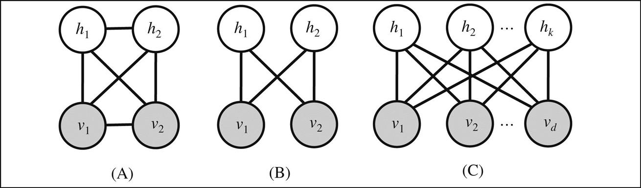
is the energy function, ![]() normalizes E so that it defines a valid joint probability, the matrices A, B, and W encode the visible-to-visible, hidden-to-hidden, and visible-to-hidden variable interactions, respectively, and vectors a and b encode the biases associated with each variable. Matrices A and B are symmetric, and their diagonal elements are 0. This structure is effectively a binary Markov random field with pairwise connections between all variables, illustrated in Fig. 10.14A.
normalizes E so that it defines a valid joint probability, the matrices A, B, and W encode the visible-to-visible, hidden-to-hidden, and visible-to-hidden variable interactions, respectively, and vectors a and b encode the biases associated with each variable. Matrices A and B are symmetric, and their diagonal elements are 0. This structure is effectively a binary Markov random field with pairwise connections between all variables, illustrated in Fig. 10.14A.
A key feature of Boltzmann machines (and binary Markov random fields in general) is that the conditional distribution of one variable given the others is a sigmoid function whose argument is a weighted linear combination of the states of the other variables:

where the notation ![]() indicates all elements with subscript other than i. The diagonal elements of A and B are zero, so there is no need for the sum to skip terms involving
indicates all elements with subscript other than i. The diagonal elements of A and B are zero, so there is no need for the sum to skip terms involving ![]() and
and ![]() , since they are zero anyway. The fact that these equations are separate sigmoid functions for each variable makes it easy to construct a Gibbs’ sampler (Section 9.5), which can be used to compute approximations to the conditional probability
, since they are zero anyway. The fact that these equations are separate sigmoid functions for each variable makes it easy to construct a Gibbs’ sampler (Section 9.5), which can be used to compute approximations to the conditional probability ![]() and the joint probability
and the joint probability ![]() .
.
Define the loss as the negative log-likelihood of the marginal probability for a single example ![]() under the Boltzmann machine model:
under the Boltzmann machine model: ![]() . Then, based on some calculus, the partial derivatives can be shown to be
. Then, based on some calculus, the partial derivatives can be shown to be

The distributions ![]() and
and ![]() needed to compute the expectations in these derivatives are not available in analytic form, but samples approximating them can be used instead. To compute the gradient of the negative log-likelihood over an entire training set with N examples, the sum of the terms is N times a single expectation using the empirical distribution of the data
needed to compute the expectations in these derivatives are not available in analytic form, but samples approximating them can be used instead. To compute the gradient of the negative log-likelihood over an entire training set with N examples, the sum of the terms is N times a single expectation using the empirical distribution of the data ![]() , or the distribution obtained by placing a delta function on each example and dividing by N. A sum over a training set involving expectations of the form
, or the distribution obtained by placing a delta function on each example and dividing by N. A sum over a training set involving expectations of the form ![]() is sometimes written as a single expectation and referred to as the data-dependent expectation, whereas the expectations involving
is sometimes written as a single expectation and referred to as the data-dependent expectation, whereas the expectations involving ![]() do not depend on the data and are referred to as the model’s expectation.
do not depend on the data and are referred to as the model’s expectation.
Using these equations and approximations for the distributions, one can implement optimization via gradient descent. Gradients in probabilistic models often come down to computing differences of expectations, as in models such as logistic regression, conditional random fields, and even probabilistic principal component analysis, as we saw in Chapter 9, Probabilistic methods.
Restricted Boltzmann Machines
Eliminating connections between hidden variables, and connections between visible variables, yields a restricted Boltzmann machine (RBM), with the same distribution ![]() but this energy function:
but this energy function:
Fig. 10.14B shows the result of this transformation on Fig. 10.14A; while Fig. 10.14C shows a more general form.
Eliminating the coupling matrices A and B means that that the exact inference step for h, the entire vector of hidden variables, can be performed in one shot. ![]() becomes the product of a different sigmoid for each dimension, each sigmoid depending only on the observed input vector v.
becomes the product of a different sigmoid for each dimension, each sigmoid depending only on the observed input vector v. ![]() has a similar form.
has a similar form.
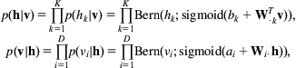
where ![]() is a vector consisting of the transpose of the kth column of the weight matrix
is a vector consisting of the transpose of the kth column of the weight matrix ![]() , while
, while ![]() is the ith row of
is the ith row of ![]() . These are conditional distributions that are derived from the underlying joint model, and the equations can be used to compute the gradient of the loss with respect to W, a, and b. The expectations needed for learning are easier to compute than for an unrestricted model: an exact expression can be obtained for
. These are conditional distributions that are derived from the underlying joint model, and the equations can be used to compute the gradient of the loss with respect to W, a, and b. The expectations needed for learning are easier to compute than for an unrestricted model: an exact expression can be obtained for ![]() , but
, but ![]() remains intractable and must be approximated.
remains intractable and must be approximated.
Contrastive Divergence
Running a Gibbs sampler for a Boltzmann machine often requires many iterations, and a technique called “contrastive divergence” is a popular alternative that initializes the sampler to the observed data instead of randomly and performs a limited number of Gibbs updates. In an RBM, a sample ![]() can be generated from the distribution
can be generated from the distribution ![]() followed by a sample for
followed by a sample for ![]() from
from ![]() . This single step often works well in practice, although the process of alternating the sampling of hidden and visible units can be continued for multiple steps.
. This single step often works well in practice, although the process of alternating the sampling of hidden and visible units can be continued for multiple steps.
Categorical and Continuous Variables
The RBMs discussed so far have been composed of binary variables. However, they can be extended to categorical or continuous attributes by encoding r=1,…, R visible categorical variables using one-hot vectors ![]() and defining hidden binary variables h with the following energy function
and defining hidden binary variables h with the following energy function
The joint distribution defined by this model is complex, but as for binary RBMs the conditional distributions under the model for one layer given the other have simple forms:
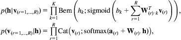
A model with a layer of continuous observed variables v and a layer of hidden binary variables h can be constructed using this energy function:
The conditional distributions are
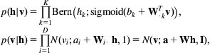
where the conditional distribution of the observed variables given the hidden is a Gaussian whose mean depends on a bias term plus a linear transformation of the binary hidden variable. This Gaussian has an identity covariance matrix and can therefore be written as a product of independent Gaussians for each dimension.
Deep Boltzmann Machines
Deep Boltzmann machines involve coupling layers of random variables using RBM connectivity, as illustrated in Fig. 10.15A. Assuming Bernoulli random variables, the energy function is

where the layers are coupled with matrices ![]() , and
, and ![]() and
and ![]() are the biases for the visible layer and each hidden layer. The gradients for the intermediate layer matrices are
are the biases for the visible layer and each hidden layer. The gradients for the intermediate layer matrices are

where the probability distributions needed for the expectations can be computed using approximate inference techniques such as Gibbs sampling or variational methods.

Examining the Markov blanket of a layer in this network shows that, given the layers above and below, variables in a given layer are independent of other layers. The conditional distribution is

This enables all variables in a layer to be updated in parallel using a method known as “block Gibbs sampling.” This is quicker than standard Gibbs sampling, but yields samples of sufficient quality for fast learning.
The overall learning procedure in deep Boltzmann machines using sampling or variational methods can be slow, and consequently greedy, incremental approaches are often used to initialize weights prior to learning. Deep Boltzmann machines can be trained incrementally by stacking two-layer Boltzmann machines, and learning the two-layer models using gradient descent and the contrastive divergence-based sampling procedure.
When training a deep RBM incrementally by stacking, to deal with the lack of top-down connections in the model, one can double the input variables of the lower-level model and constrain the associated matrix to be the same as the original; double the output variables of the higher-level model and constrain its matrix in the same way. Once the first Boltzmann machine has been learned, the next can be learned using either a sample from independent Bernoulli distributions for the dimensions of ![]() based on the sigmoid models of the rewritten Boltzmann machine, or using the value of the sigmoid activations. In both cases a fast approximate inference upward pass can be performed using a doubled weight matrix to compensate for the fact that the top-down influence of the model is not captured. When generating a sampler or sigmoid activity for the final layer, it is not necessary to double the weights. Subsequent levels can be learned similarly.
based on the sigmoid models of the rewritten Boltzmann machine, or using the value of the sigmoid activations. In both cases a fast approximate inference upward pass can be performed using a doubled weight matrix to compensate for the fact that the top-down influence of the model is not captured. When generating a sampler or sigmoid activity for the final layer, it is not necessary to double the weights. Subsequent levels can be learned similarly.
Deep Belief Networks
While any deep Bayesian network is technically a deep belief network, the term “deep belief network” has become strongly associated with a particular type of deep architecture that can be constructed by training RBMs incrementally. The procedure is based on converting the lower part of a growing model into a Bayesian belief network, adding an RBM for the upper part of the model, then continuing the training, conversion, and stacking process. As we have seen above, an RBM is a two-layer joint model for which we can use some algebra to write conditional models of observed given hidden, or hidden given observed layers that are consistent with the underlying joint distribution. It therefore follows that a deep belief network can be obtained through a procedure of learning a joint RBM model for two layers, converting the model into its conditional formulation for the layer below given the layer above, then adding a new layer on top to the model, parameterizing the top two layers as a new joint RBM model, then learning the new parameters. Fig. 10.15B illustrates the general form, which can be written
where as before the model is defined in terms of a visible layer ![]() and l=l,…,L hidden layers
and l=l,…,L hidden layers ![]() . The conditional distributions are all products of Bernoulli distributions with sigmoidal parameterizations.
. The conditional distributions are all products of Bernoulli distributions with sigmoidal parameterizations.
The top two layers are parameterized as an RBM. If they have directed rather than undirected connections, they can be decomposed into the form ![]() , where the conditional distribution is another sigmoidally parameterized Bernoulli product and
, where the conditional distribution is another sigmoidally parameterized Bernoulli product and ![]() is the product over a separate distribution for each
is the product over a separate distribution for each ![]() . The result is known as a deep sigmoidal belief network.
. The result is known as a deep sigmoidal belief network.
The network shown in Fig. 10.15B can be constructed and trained in a layer-by-layer manner. To see this, consider a RBM with visible variables ![]() and two layers of hidden variables
and two layers of hidden variables ![]() followed by
followed by ![]() on top. A joint model for
on top. A joint model for ![]() can be defined as either a 3-layer Boltzmann machine, or, by restructuring the parameterization of the lower two layers, as a belief network with an RBM at the top using
can be defined as either a 3-layer Boltzmann machine, or, by restructuring the parameterization of the lower two layers, as a belief network with an RBM at the top using
(10.2)
 (10.2)
where ![]() has the usual form
has the usual form

and the parameters ![]() and
and ![]() of
of ![]() are independent of the parameters
are independent of the parameters ![]() ,
, ![]() , and
, and ![]() of
of ![]() .
.
Such networks can be trained as follows: first train a 2-layer Boltzmann machine using the observed data. Then add a layer on top, and initialize its weights to the transpose of the weights learned in the layer below. To train the next layer, compute the conditional distribution for the layer above given the layer below, and either generate a sample or use the activation of the sigmoid function to transform each example of the training data into the first hidden layer representation. The properties of a RBM can be further exploited to obtain the conditional distribution of the lower layer given the upper layer, and the parameters of the conditional model in this direction can be fixed. Once the second Boltzmann machine has been trained, the model has the form (Eq. 10.2), and the process of transforming the data, transforming the top-level Boltzmann machine into a conditional model, adding a layer, and training a top layer Boltzmann machine can be repeated as desired.
If the layer above has a different number of units, the transpose of the matrix below cannot be used for initialization and certain theoretical guarantees no longer apply. However, in practice the procedure is known to work well with random initialization.
10.6 Recurrent Neural Networks
Recurrent neural networks are networks with connections that form directed cycles. As a result, they have an internal state, which makes them prime candidates for tackling learning problems involving sequences of data—such as handwriting recognition, speech recognition, and machine translation. Fig. 10.16A shows how a feedforward network can be transformed into a recurrent network by adding connections from all hidden units hi to hj. Each hidden unit has connections to both itself and other hidden units.

Imagine unfolding a recurrent network over time by following the sequence of steps that perform the underlying computation. Like a hidden Markov model, a recurrent network can be unwrapped and implemented using the same weights and biases at each step to link units over time. Fig. 10.16B shows a hidden Markov model unfolded in time and written as a dynamic Bayesian network, while Fig. 10.16C shows a recurrent network obtained by unwrapping Fig. 10.16A. Recurrent neural networks operate in a deterministic continuous space, in contrast to hidden Markov models, which generally utilize discrete random variables. Whereas it is common to think of deep feedforward networks as computing more abstract features as one progresses up the network, information processing in recurrent networks proceeds more like steps in the execution of a more general algorithm.
Recurrent neural networks, and the particular discussed below—known as “long short-term memory” (LSTM) recurrent neural networks—have been particularly successful for many tasks, from unconstrained handwriting recognition to speech recognition and machine translation.
These networks apply linear matrix operations to the current observation and the hidden units from the previous time step, and the resulting linear terms serve as arguments of activation functions act():
(10.3)
The same matrix ![]() is used at each time step. Through it, the hidden units in the previous step
is used at each time step. Through it, the hidden units in the previous step ![]() influence the computation of
influence the computation of ![]() , while the current observation contributes a term
, while the current observation contributes a term ![]() term that is summed with
term that is summed with ![]() and a bias term
and a bias term ![]() . Both
. Both ![]() and
and ![]() are typically replicated over time. The output layer is modeled by a classical neural network activation function applied to a linear transformation of the hidden units, and the operation is replicated at each time step.
are typically replicated over time. The output layer is modeled by a classical neural network activation function applied to a linear transformation of the hidden units, and the operation is replicated at each time step.
The loss for a particular sequence in the training data can be computed either at each time step or just once, at the end of the sequence. In either case, predictions will be made after many processing steps. This brings us to an important problem. Eq. (10.1) for feedforward networks decomposes the gradient of parameters at layer l into a product of matrix multiplications of the form ![]() . A recurrent network uses the same matrix at each time step, and over many steps the gradient can very easily either diminish to zero or explode to infinity—just as the magnitude of any number (other than one) taken to a large power either approaches zero or increases indefinitely.
. A recurrent network uses the same matrix at each time step, and over many steps the gradient can very easily either diminish to zero or explode to infinity—just as the magnitude of any number (other than one) taken to a large power either approaches zero or increases indefinitely.
Exploding and Vanishing Gradients
The use of L1 or L2 regularization can mitigate the problem of exploding gradients by encouraging weights to be small. Another strategy is to simply detect if the norm of the gradient exceeds some threshold and, if so, scale it down. This is sometimes called gradient (norm) clipping. That is, for a gradient vector ![]() and threshold T,
and threshold T,

T is a hyperparameter, which can be set to the average norm over several previous updates where clipping was not used.
The so-called “LSTM” recurrent neural network architecture was specifically created to address the vanishing gradient problem. It uses a special combination of hidden units, elementwise products and sums between units to implement gates that control “memory cells.” These cells are designed to retain information without modification for long periods of time. They have their own input and output gates, which are controlled by learnable weights that are a function of the current observation and the hidden units at the previous time step. As a result, backpropagated error terms from gradient computations can be stored and propagated backwards without degradation. The original LSTM formulation consisted of input gates and output gates, but forget gates and “peephole weights” were added later. The architecture is complex, but has produced state-of-the-art results on a wide variety of problems. Below we present the most popular variant of LSTM RNNs, which does not include peephole weights but does use forget gates.
LSTM RNNs work as follows: at each time step there are three types of gate, input ![]() , forget
, forget ![]() , and output
, and output ![]() , each being a function of the underlying input
, each being a function of the underlying input ![]() at time t and the hidden units at time t–1,
at time t and the hidden units at time t–1, ![]() . Gates multiply
. Gates multiply ![]() by their own gate-specific W matrix
by their own gate-specific W matrix ![]() , by their own U matrix, and add their own bias vector b, followed by the application of a sigmoidal elementwise nonlinearity.
, by their own U matrix, and add their own bias vector b, followed by the application of a sigmoidal elementwise nonlinearity.
At each time step t, input gates ![]() are used to determine whether a potential input given by
are used to determine whether a potential input given by ![]() is sufficiently important to be placed into the memory unit
is sufficiently important to be placed into the memory unit ![]() . The computation of
. The computation of ![]() itself is a linear combination of the current input value
itself is a linear combination of the current input value ![]() and the previous hidden unit vector
and the previous hidden unit vector ![]() , using weight matrices
, using weight matrices ![]() and
and ![]() along with a bias vector
along with a bias vector ![]() . Forget gates
. Forget gates ![]() allow the content of memory units to be erased using
allow the content of memory units to be erased using ![]() , involving a similar linear input based on
, involving a similar linear input based on ![]() and
and ![]() matrices, plus a bias
matrices, plus a bias ![]() . Output gates
. Output gates ![]() determine whether
determine whether ![]() , the content of the memory units transformed by activation functions, should be placed in the hidden units
, the content of the memory units transformed by activation functions, should be placed in the hidden units ![]() . They are typically controlled by a sigmoidal activation function
. They are typically controlled by a sigmoidal activation function ![]() applied to a linear combination of the current input value
applied to a linear combination of the current input value ![]() and the previous hidden unit vector
and the previous hidden unit vector ![]() , using weight matrices
, using weight matrices ![]() and
and ![]() along with a bias vector
along with a bias vector ![]() .
.
This final gating is implemented as an elementwise product between the output gate and the transformed memory contents, ![]() , where memory units are typically transformed by the tanh function prior to the gated output:
, where memory units are typically transformed by the tanh function prior to the gated output: ![]() . Memory units are updated by
. Memory units are updated by ![]() , an elementwise product between the forget gates
, an elementwise product between the forget gates ![]() and the previous contents of the memory units
and the previous contents of the memory units ![]() , plus the elementwise product of the input gates
, plus the elementwise product of the input gates ![]() , and the new potential inputs
, and the new potential inputs ![]() . Table 10.5 defines these components, and Fig. 10.17 shows a computation graph for the intermediate quantities.
. Table 10.5 defines these components, and Fig. 10.17 shows a computation graph for the intermediate quantities.


Other Recurrent Network Architectures
A wide variety of other recurrent network architectures have been proposed. For example, the network given by Eq. (10.3) can be used with rectified linear activation functions, using scaled versions of the identity matrix to initialize the recurrent weight matrix, and initializing biases to zero. The identity initialization means that error derivatives flow through the network unmodified. Initializing with smaller, scaled versions of the identity matrix has the effect of causing the model to forget longer range dependencies. This approach is known as an IRNN. Another possibility is to simplify LSTM networks by dispensing with separate memory cells and using gated recurrent units or GRUs. For some problems GRUs can provide performance comparable with LSTMs, but with a lower memory requirement.
Recurrent networks can be made bidirectional, propagating information in both directions: Fig. 10.18A shows the general structure. Bidirectional networks have been used for a wide variety of applications, including protein secondary structure prediction and handwriting recognition. Modern software tools determine the gradients required for learning via backpropagation automatically, by manipulating computation graphs.

Fig. 10.18B shows an “encoder-decoder” network. Such networks allow the creation of fixed-length vector representations for variable-length inputs, and can use the fixed-length encoding to generate another variable-length sequence as the output. This is particularly useful for machine translation, where the input is a string in one language and the output is the corresponding string in another language. Given enough data, a deep encoder-decoder architecture such as that of Fig. 10.19 can yield results that compete with those of systems that have been hand-engineered over decades of research. The connectivity structure means that partial computations in the model can flow through the graph in a wave, illustrated by the darker nodes in the figure.

10.7 Further Reading and Bibliographic Notes
The backpropagation algorithm has been known in close to its current form since Werbos’ (1974) PhD thesis; in his extensive literature review of deep learning, Schmidhuber (2015) traces key elements of the algorithm back even further. He also traces the idea of “deep networks” back to the work of Ivakhnenko and Lapa (1965). Modern CNNs are widely acknowledged as having their roots with the “neocognitron” proposed by Fukushima (1980). However, the work of LeCun, Bottou, Bengio, and Haffner (1998) on the LeNet convolutional network architecture has been extremely influential.
The popularity of neural network techniques has gone through several cycles. While some factors are social, there are important technical reasons behind the trends. A single-layer neural network cannot solve the XOR problem, a failing that was derided by Minsky and Papert (1969) which, as mentioned in Section 4.10, stymied neural network development until the mid-1980s. However, it is well known that networks with one additional layer can approximate any function (Cybenko, 1989; Hornik, 1991), and Rumelhart, Hinton, and Williams’ (1986) influential work repopularized neural network methods for a while. However, by the early 2000s they had fallen out of favor again. Indeed, the organizers of NIPS, the Neural Information Processing Systems conference, which was (and still is) widely considered to be the premier forum for neural network research, found that the presence of the term “neural networks” in the title was highly correlated with the paper’s rejection!—a fact that is underscored by citation analysis of key neural network papers during this period. The recent resurgence of interest in deep learning really does feel like a “revolution.”
It is known that most complex Boolean functions require an exponential number of two-step logic gates for their representation (Wegener, 1987). The solution appears to be greater depth: according to Bengio (2009), the evidence strongly suggests that “functions that can be compactly represented with a depth-k architecture could require a very large number of elements in order to be represented by a shallower architecture.”
Many neural network books (Haykin, 1994; Bishop, 1995; Ripley, 1996) do not formulate backpropagation in vector-matrix terms. However, recent online courses (e.g., by Hugo Larochelle), and Rojas’ (1996) text, do adopt this formulation, as we have done in this chapter.
Stochastic gradient descent methods go back at least as far as Robbins and Monro (1951). Bottou (2012) is an excellent source of tips and tricks for learning with stochastic gradient descent, while Bengio (2012) gives further practical recommendations for training deep networks. Bergstra and Bengio (2012) give empirical and theoretical justification for the use of random search for hyperparameter settings. Snoek, Larochelle, and Adams (2012) propose the use of Bayesian learning methods to infer the next hyperparameter setting to explore, and their Spearmint software package performs Bayesian optimizations of both deep network hyperparameters and general machine learning algorithm hyperparameters.
Good parameter initialization can be critical for the success of neural networks, as discussed in LeCun et al.’s (1998) classic work and the more recent work of Glorot and Bengio (2010). Krizhevsky et al.’s (2012) convolutional network of ReLUs initialized weights using 0-mean isotropic Gaussian distributions with a standard deviation of 0.01, and initialized the biases to 1 for most hidden convolutional layers as well as the model’s hidden fully connected layers. They observed that this initialization accelerated the early phase of learning by providing ReLUs with positive inputs.
The origins of dropout and more details about it can be found in Srivastava, Hinton, Krizhevsky, Sutskever, and Salakhutdinov (2014). Ioffe and Szegedy (2015) proposed batch normalization and give more details on its implementation. Glorot and Bengio (2010) cover various weight matrix initialization heuristics, and how the concepts of fan-in and fan-out can be used to justify them for networks with different kinds of activation functions.
The MNIST data set containing 28×28 pixel images of handwritten digits has been popular for exploring ideas in the deep learning research community. However, it was the ImageNet challenge, with a variety of much higher resolutions, that catapulted deep learning into the spotlight in 2012 (Russakovsky et al., 2015). The winning entry from the University of Toronto processed the images at a resolution of 256×256 pixels. Up till then, CNNs were simply incapable of processing such large volumes of imagery at such high resolutions in a reasonable amount of time. Krizhevsky et al.’s (2012) dramatic win used a GPU-accelerated CNNs. This spurred a great deal of development, reflected in rapid subsequent advances in visual recognition performance on the ImageNet benchmark.
In the 2014 challenge, the Oxford Visual Geometry Group and a team from Google pushed performance even further using much deeper architectures: 16–19 weight layers for the Oxford group, using tiny 3×3 convolutional filters (Simonyan and Zisserman, 2014); 22 layers, with filters up to 5×5 for the Google team (Szegedy et al., 2015). The 2015 ImageNet challenge was won by a team from Microsoft Research Asia using an architecture with 152 layers (He et al., 2015), using tiny 3×3 filters combined with shortcut connections that skip over layers, they also perform pooling and decimation after multiple layers of convolution have been applied.
Hinton and Salakhutdinov (2006) noted that it has been known since the 1980s that deep autoencoders, optimized through backpropagation, could be effective for nonlinear dimensionality reduction. The key limiting factors were the small size of the data sets used to train them, coupled with low computation speeds: plus the old problem of local minima. By 2006, data sets such as the MNIST digits and the 20 Newsgroups collection were large enough, and computers were fast enough, for Hinton and Salakhutdinov to present compelling results illustrating the advantages of deep autoencoders over principal component analysis. Their experimental work used generative pretraining to initialize weights to avoid problems with local minima.
Bourlard and Kamp (1988) provide a deep analysis of the relationships between autoencoders and principal component analysis. Vincent, Larochelle, Lajoie, Bengio, and Manzagol (2010) proposed stacked denoising autoencoders and found that they outperform both stacked standard autoencoders and models based on stacking RBMs. Cho and Chen (2014) produced state-of-the-art results on motion capture sequences by training deep autoencoders with rectified linear units using hybrid unsupervised and supervised learning.
The history of Markov random fields has roots in statistical physics in the 1920s with so-called “Ising models” of ferromagnetism. Our presentation of Boltzmann machines follows Hinton and Sejnowski (1983), but we use matrix-vector notation and our exposition more closely resembles formulations such as that of Salakhutdinov and Hinton (2009). Harmonium networks proposed in Smolensky (1986) are essentially equivalent to what are now commonly referred to as RBMs.
Contrastive divergence was proposed by Hinton (2002). The idea of using unsupervised pretraining to initialize deep networks using stacks of RBMs was popularized by Hinton and Salakhutdinov (2006); Salakhutdinov and Hinton (2009) give further details on the use of deep Boltzmann machines and training procedures for deep belief networks, including the variable doubling procedure and other nuances discussed above for greedy training of deep restricted Boltzmann machines. Neal (1992) introduced sigmoidal belief networks. Welling, Rosen-Zvi, and Hinton (2004) showed how to extend Boltzmann machines to categorical and continuous variables using exponential-family models. The greedy layerwise training procedure for deep Boltzmann machines in Section 10.4 is based on a procedure proposed by Hinton and Salakhutdinov (2006) and refined by Murphy (2012).
Hybrid supervised and unsupervised learning procedures for restricted Boltzmann machines were proposed by McCallum, Pal, Druck, and Wang (2006) and further explored by Larochelle and Bengio (2008). Vincent et al. (2010) proposed the autoencoder approach to unsupervised pretraining; they also explored various layerwise stacking and training strategies and compared stacked RBMs with stacked autoencoders.
Graves et al. (2009) demonstrate how recurrent neural networks are particularly effective at handwriting recognition, while Graves, Mohamed, and Hinton (2013) apply recurrent neural networks to speech. The form of gradient clipping presented in Section 10.6 was proposed by Pascanu, Mikolov, and Bengio (2013).
The vanishing gradient problem was formally identified as a key issue for learning in deep networks by Sepp Hochreiter in his diploma thesis (Hochreiter, 1991). The impact in terms of the difficulty of learning long-term dependencies is discussed by Bengio, Simard, and Frasconi (1994). Further analysis of the issue is given by Hochreiter, Bengio, Frasconi, and Schmidhuber (2001).
Hochreiter and Schmidhuber (1997) is the seminal paper on the “long short-term memory” architecture for recurrent neural networks; our explanation follows Graves and Schmidhuber (2005)’s formulation. Greff, Srivastava, Koutník, Steunebrink, and Schmidhuber’s (2015) paper “LSTM: A search space odyssey” explored a wide variety of variants and finds that: (1) none of them significantly outperformed the standard LSTM architecture; and (2) forget gates and the output activation function were the most critical components. Forget gates were added by Gers, Schmidhuber, and Cummins (2000).
IRNNs were proposed by Le, Jaitly, and Hinton (2015), while Chung, Gulcehre, Cho, and Bengio (2014) proposed gated recurrent units and Schuster and Paliwal (1997) proposed bidirectional recurrent neural networks. Chen and Chaudhari (2004) used bidirectional networks for protein structure prediction, while Graves et al. (2009) used them for handwriting recognition. Cho et al. (2014) used encoder-decoder networks for machine translation, while Sutskever, Vinyals, and Le (2014) proposed deep encoder-decoder networks and used them with massive quantities of data.
For further accounts of advances in deep learning and a more extensive history of the field, consult the reviews of LeCun, Bengio, and Hinton (2015), Bengio (2009), and Schmidhuber (2015).
10.8 Deep Learning Software and Network Implementations
Theano
Theano is a library in the Python programming language that has been developed with the specific goal of facilitating research in deep learning (Bergstra et al., 2010; Theano Development Team, 2016). It is also a powerful general purpose tool for mathematical programming. Theano extends NumPy (the fundamental Python package for scientific computing) by adding symbolic differentiation and GPU support, among various other functions. It provides a high-level language for creating the mathematical expressions that underlie deep learning models, and a compiler that takes advantage of deep learning techniques, and calls to GPU libraries, to produce code that executes quickly. Theano supports execution on multiple GPUs. It allows the user to declare symbolic variables for inputs and targets, and supply numerical values only when they are used. Shared variables such as weights and biases are associated with numerical values stored in NumPy arrays. Theano creates symbolic graphs as a result of defining mathematical expressions involving the application of operations to variables. These graphs consist of variable, constant, apply, and operation nodes. Constants, and constant nodes, are a subclass of variables, and variable nodes, which hold data that will remain constant—and can therefore be subjected to various optimizations by the compiler. Theano is an open-source project using a BSD license.
Tensor Flow
Tensor Flow is a C++ and Python-based software library for the types of numerical computation typically associated with deep learning (Abadi et al., 2016). It is heavily inspired by Theano and, like it, uses dataflow graphs to represent the ways in which multidimensional data arrays communicate between one another. These multidimensional arrays are referred to as “tensors.” Tensor Flow also supports symbolic differentiation and execution on multiple GPUs. It was released in 2015 and is available under the Apache 2.0 license.
Torch
Torch is an open-source machine learning library built using C and a high-level scripting language known as Lua (Collobert, Kavukcuoglu, & Farabet, 2011). It uses multidimensional array data structures, and supports various basic numerical linear algebra manipulations. It has a neural network package with modules that permit the typical forward and backward methods needed for training neural networks. It also supports automatic differentiation.
Computational Network Toolkit
The Computational Network Toolkit (CNTK) is a C++ library for manipulating computational networks (Yu et al., 2014). It was produced by Microsoft Research, but has been released under a permissive license. It has been popular for speech and language processing, but also supports convolutional networks of the type used for images. It supports execution on multiple machines and using multiple GPUs.
Caffe
Caffe is a C++ and Python-based BSD-licensed CNN library (Jia et al., 2014). It has a clean and extensible design that makes it a popular alternative to the original open-source implementation of Krizhevsky et al.’s (2012) famous AlexNet that won the 2012 ImageNet challenge.
Deeplearning4j
Deeplearning4j is a Java-based open-source deep learning library available under the Apache 2.0 license. It uses an multidimensional array class and provides linear algebra and matrix manipulation support similar to that provided by Numpy.
Other Packages: Lasagne, Keras, and cuDNN
Lasagne is a lightweight Python library built on top of Theano that simplifies the creation of neural network layers. Similarly, Keras is a Python library that runs on top of either Theano or TensorFlow (Chollet, 2015). It allows one to quickly define a network architecture in terms of layers and also includes functionality for image and text preprocessing. cuDNN is a highly optimized GPU library for NVIDIA units that allows deep networks to be trained more quickly. It can dramatically accelerate the performance of a deep network and is often called by the other packages above.
10.9 WEKA Implementations
Deep learning can be implemented in WEKA using three methods:
• With the wrapper classifier for the third-party DeepLearningForJ package that is available in the deepLearningForJ package.
• Using the MLRClassifier from the RPlugin package to exploit deep learning implementations in R.
• By accessing Python-based deep learning libraries using the PyScript package.