The MNIST Evaluation

To underscore the importance of large benchmark evaluations, consider the Mixed National Institute of Standards and Technology (MNIST) database of handwritten digits. It contains 60,000 training and 10,000 test instances of hand-written digits, encoded as 28×28 pixel grayscale images. The data is a remix of an earlier NIST data set in which adults generated the training data and high school students generated the test set. Table 10.1 gives some results on this data. Note that the LeNet convolutional network (row 5), a deep architecture discussed in Section 10.3, outperformed many standard machine learning techniques, even in 1998.

The lower half of the table shows the results of methods that augment the training set with synthetic distortions of the input images. The use of transformations to further extend the size of an already large data set is an important technique in deep learning. Large networks, with more parameters, have high representational capacity. Plausible synthetic distortion of the data multiplies the amount of data available, preventing overfitting and helping the network to generalize. Of course, other methods such as support vector machines can also scale up model complexity with additional data. Simply adding more support vectors can allow SVM-based methods to outperform classical network architectures. However, as Table 10.1 shows, training deep feedforward networks or CNN with synthetic elastically transformed imagery yields even better results. Because of the large test set, differences in the error rate of more than 0.01 are statistically significant.

The last four entries illustrate the effectiveness of deep networks. Interestingly, a standard multilayer perceptron with six layers using synthetic transformations and trained on a graphics processing unit matches the performance of a large and deep CNN. This shows that plain neural networks can be effective when they are deep and data augmentation is used, because training such a network with synthetically transformed data encourages robustness with respect to plausible distortions. In contrast, CNNs embed translational invariances within the network design itself (see Section 10.3). The best result in Table 10.1 is based on an ensemble of convolutional networks. Ensembles are used to obtain the top performance in many settings.

Losses and Regularization

Section 7.2 noted that different activation functions can be used for multilayer perceptrons. We distinguish the final-layer parameterization, from which the loss function is computed, from the intermediate-layer activation functions. In the past, it was common practice to use sigmoids as output activation functions and base final-layer loss functions on squared errors—sometimes even when classification labels were constrained to be 0 or 1. Later designs, however, embrace the natural probabilistic encoding for any given data type by defining output activation functions as the negative log of the distribution functions used to make probabilistic predictions, whether these distributions are binary, categorical, or continuous. Then predictions can correspond precisely to the underlying probability models defined by Bernoulli, discrete or Gaussian distributions—as in linear and logistic regression, but with greater flexibility.

Viewed in this way, logistic regression is a simple neural network with no hidden units. The underlying optimization criterion for predicting i=1,…, N labels y_i from features x_i with parameters $\theta$ consisting of a matrix of weights W and a vector of biases b is

$\sum _{i=1}^N-\log p(y_i|{\mathbf{x}}_i;\mathbf{W},\mathbf{b})+\lambda \sum _{j=1}^M{w}_j^2=\sum _{i=1}^{N}L(f_i({\mathbf{x}}_i;\theta ),y_i)+\lambda R(\theta )$

where the first term, $L(f_i({\mathbf{x}}_i;\theta ),y_i)$, is the negative conditional log-likelihood or loss, and the second, $\lambda R(\theta )$, is a weighted regularizer used to prevent overfitting.

This formulation as a loss- and regularizer-based objective function gives us the freedom to choose either probabilistic losses or other loss functions dictated by the needs of the application. Using the average loss over the training data, called the empirical risk, leads to the following formulation of the fundamental optimization problem posed by training a deep model: minimize the empirical risk plus a regularization term, i.e.,

$\underset{\theta }{\arg \min }\left[\frac{1}{N}\sum _{i=1}^{N}L\left(f_i\right({\mathbf{x}}_i;\theta ),{\mathbf{y}}_i)+\lambda R\left(\theta \right)\right].$

Note that the factor N must be accounted for if one relates the regularization weight $\lambda$ here to the corresponding parameter derived from a formal probabilistic model for the distribution. In deep learning we are often interested in examining learning curves that show the loss or some other performance metric on a graph as a function of the number of passes that an algorithm has taken over the data. It is much easier to compare the average loss over a training set with the average loss over a validation set on the same graph, because dividing by N gives them the same scale.

To see how deep networks learn, consider composing the final output function of a network in which $f_k(\mathbf{x})=f_k(a_k(\mathbf{x}))$. This function is applied to an input activation consisting of $a_k(\mathbf{x})$. The input frequently comprises a computation of the form $\mathbf{a}(\mathbf{x})=\mathbf{W}\mathbf{h}(\mathbf{x})+\mathbf{b}$, where function a(x) takes a vector argument and returns a vector as its result, so that $a_k(\mathbf{x})$ is just one of the elements of a(x). Table 10.2 gives commonly used output loss functions, output activation functions, and underlying distributions from which they derive.

Table 10.2

Loss Functions, Corresponding Distributions, and Activation Functions

Loss Name, $L(f_i({\mathbf{x}}_i;\theta ),{\mathbf{y}}_i)=$	Distribution Name, $P(f_i({\mathbf{x}}_i;\theta ),{\mathbf{y}}_i)=$	Output Activation Function, $f_k(a_k(\mathbf{x}))=$
Squared error, ${\sum }_{k=1}^K{(f_k(\mathbf{x})-y_k)}^2$	Gaussian, $N(\mathbf{y};\mathbf{f}(\mathbf{x};\theta ),\mathbf{I})$	$\frac{1}{(1+\exp (-a_k(\mathbf{x})))}$
Cross entropy, $-{\sum }_{k=1}^K\left[y_k\log f_k(\mathbf{x})+(1-y_k)\log (1-f_k(\mathbf{x}))\right]$	Bernoulli, $\mathrm{Bern}(\mathbf{y};\mathbf{f}(\mathbf{x};\theta ))$	$\frac{1}{(1+\exp (-a_k(\mathbf{x})))}$
Categorical cross entropy, $-{\sum }_{k=1}^K{y}_k\log f_k(\mathbf{x})$	Discrete or Categorical, $\mathrm{Cat}(\mathbf{y};\mathbf{f}(\mathbf{x};\theta ))$	$\frac{\exp (a_k(\mathbf{x}))}{{\sum }_{j=1}^K\exp (a_j(\mathbf{x}))}$

Deep Layered Network Architecture

Deep neural networks compose computations performed by many layers. Denoting the output of hidden layers by h^(l)(x), the computation for a network with L hidden layers is:

$\mathbf{f}(\mathbf{x})=\mathbf{f}\left[{\mathbf{a}}^{(L+1)}\left({\mathbf{h}}^{(L)}\left({\mathbf{a}}^{(L)}\left(\dots \left({\mathbf{h}}^{(2)}\left({\mathbf{a}}^{(2)}\left({\mathbf{h}}^{(1)}\left({\mathbf{a}}^{(1)}(\mathbf{x})\right)\right)\right)\right)\right)\right)\right)\right].$

Each preactivation function a^(l)(x) is typically a linear operation with matrix W^(l) and bias b^(l), which can be combined into a parameter θ:

$\begin{array}{c}{\mathbf{a}}^{(l)}(\mathbf{x})={\mathbf{W}}^{(l)}\mathbf{x}+{\mathbf{b}}^{(l)},\\ {\mathbf{a}}^{(l)}(\stackrel{\mathbf{ˆ}}{\mathbf{x}})={\mathbf{\theta }}^{(l)}\stackrel{\mathbf{ˆ}}{\mathbf{x}},l=1\\ {\mathbf{a}}^{(l)}({\stackrel{\mathbf{ˆ}}{\mathbf{h}}}^{(l-\mathrm{1})})={\mathbf{\theta }}^{(l)}{\stackrel{\mathbf{ˆ}}{\mathbf{h}}}^{(l-\mathrm{1})},l>1\end{array}$

The “hat” notation $\stackrel{\mathbf{ˆ}}{\mathbf{x}}$ indicates that 1 has been appended to the vector x. Hidden-layer activation functions h^(l)(x) often have the same form at each level, but this is not a requirement.

Fig. 10.1 shows an example network. In contrast to graphical models such as Bayesian networks where hidden variables are random variables, the hidden units here are intermediate deterministic computations, which is why they are not represented as circles. However, the output variables y_k are drawn as circles because they can be formulated probabilistically.

Activation Functions

Activation functions generally operate on the preactivation vectors in an elementwise fashion.

Table 10.3 depicts common hidden-layer activation functions, along with their functional forms and derivatives.

Table 10.3

Activation Functions and Their Derivatives

Name and Graph	Function	Derivative
	$h(x)=\frac{1}{1+\exp (-x)}$	$h\text{'}(x)=h(x)\left[1-h(x)\right]\begin{array}{c}\\ \end{array}$
	$h(x)=\frac{\exp (x)-\exp (-x)}{\exp (x)+\exp (-x)}$	$h\text{'}(x)=1-h{(x)}^2\begin{array}{c}\\ \end{array}$
	$h(x)=\log (1+\exp (x))\begin{array}{c}\\ \end{array}$	$h\text{'}(x)=\frac{1}{1+\exp (-x)}$
	$h(x)=\max (0,x)\begin{array}{c}\\ \end{array}$	$h\text{'}(x)=\{\begin{array}{c}1\\ 0\end{array}\begin{array}{c}\mathrm{if}x\ge 0\\ \mathrm{if}x<0\end{array}$
	$h(x)=\{\begin{array}{c}x\\ ax\end{array}\begin{array}{c}\mathrm{if}x\ge 0\\ \mathrm{if}x<0\end{array}$	$h\text{'}(x)=\{\begin{array}{c}1\\ a\end{array}\begin{array}{c}\mathrm{if}x\ge 0\\ \mathrm{if}x<0\end{array}$

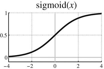
While sigmoid functions have been popular, the hyperbolic tangent function is sometimes preferred, partly because it has a steady state at 0. However, more recently the rectify() function or rectified linear units (ReLUs) have been found to yield superior results in many different settings. Since this function is 0 for negative argument values, some units in the model will yield activations that are 0, giving a “sparseness” property that is useful in many contexts. Moreover, the gradient is particularly simple—either 0 or 1. The fact that when activated, the activation function has a gradient of exactly 1 helps address the vanishing or exploding gradient problem—we discuss this in more detail below, under recurrent networks. ReLUs are a popular choice for h^(l)(x), while piecewise linear functions (the last entry of Table 10.3) have also grown in popularity for deep learning systems. Like ReLUs, these are not differentiable at 0, but gradient descent can be applied by using a subgradient instead, which means that $h\prime \left(0\right)$ can be set to a (e.g.).

Many deep learning software packages make it easy to use a variety of activation functions, including piecewise-linear ones. Some determine the gradients needed for the backpropagation algorithm automatically, using symbolic computations built into the software.

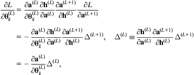
Fig. 10.2 is a computation graph that shows the general form of a canonical deep network architecture with several hidden layers. It illustrates how predictions are computed, how the loss L is obtained, and how the forward pass of the backpropagation algorithm is computed. Hidden-layer activation functions are given by act (a^(l)), and the final layer activation function is given by out (a^(L+1)).

Backpropagation Revisited

Backpropagation is based on the chain rule of calculus. Consider the loss $L(\mathbf{f}(\mathbf{x};\theta ),\mathbf{y})$ for a single-layer network with a softmax output that corresponds exactly to the model for multinomial logistic regression. We use multinomial vectors y, with a single dimension y_k=1 for the corresponding class label and whose other dimensions are 0. Define $\mathbf{f}=\left[\begin{array}{ccc}{f}_1\left(\mathbf{a}\right),& \dots ,& f_K\left(\mathbf{a}\right)\end{array}\right]$, and $\mathbf{a}(\mathbf{x};\mathbf{\theta })=\left[\begin{array}{ccc}{a}_1(\mathbf{x};{\mathbf{\theta }}_1),& \dots ,& a_K(\mathbf{x};{\mathbf{\theta }}_K)\end{array}\right]$ with $a_k(\mathbf{x};{\mathbf{\theta }}_k)={\mathbf{\theta }}_k^T\mathbf{x}$, where ${\mathbf{\theta }}_k$ is a column vector containing the k^th row of the parameter matrix $\mathbf{\theta }$. A softmax loss for $\mathbf{f}(\mathbf{a}(\mathbf{x}))$ is given by

$L=-\sum _{k=1}^K{y}_k\log f_k(\mathbf{x}),f_k(\mathbf{x})=\frac{\exp (a_k(\mathbf{x}))}{{\sum }_{c=1}^K\exp (a_c(\mathbf{x}))}.$

To replicate a model of the form $a_k(\mathbf{x};{\mathbf{w}}_k,\mathbf{b})={\mathbf{w}}_k^T\mathbf{x}+\mathbf{b}$, define x to include a 1 at the end, so that the bias parameter b is the last element of each parameter vector ${\mathbf{\theta }}_k$. The chain rule in vector form gives the partial derivative with respect to any given parameter vector ${\mathbf{\theta }}_k$ as

$\frac{\partial L}{\partial {\mathbf{\theta }}_k}=\frac{\partial \mathbf{a}}{\partial {\mathbf{\theta }}_k}\frac{\partial \mathbf{f}}{\partial \mathbf{a}}\frac{\partial L}{\partial \mathbf{f}}=\frac{\partial \mathbf{a}}{\partial {\mathbf{\theta }}_k}\frac{\partial L}{\partial \mathbf{a}}.$

(Note that the order of terms is reversed compared to earlier applications of the chain rule in this book.)

For each component of the partial derivative of the loss with respect to a,

$\begin{array}{ll}\frac{\partial L}{\partial a_j}\hfill & =\frac{\partial }{\partial a_j}\left[-\sum _{k=1}^K{y}_k\left[a_k-\log \left[\sum _{c=1}^K\exp (a_c)\right]\right]\right]\hfill \\ \hfill & =-\left[y_{k=j}-\frac{\exp (a_{k=j})}{{\sum }_{c=1}^K\exp (a_c)}\right]\hfill \\ \hfill & \mathbf{=}-\left[y_j-p(y_j|\mathbf{x})\right]\hfill \\ \hfill & =-\left[y_j-f_j(\mathbf{x})\right],\hfill \end{array}$

which implies that the vector form can be written

$\frac{\partial L}{\partial \mathbf{a}}=-[\mathbf{y}-\mathbf{f}(\mathbf{x})],$

where $\mathrm{\Delta }=[\mathbf{y}-\mathbf{f}(\mathbf{x})]$ is often referred to as the error.

Next, since

$\frac{\partial a_j}{\partial {\mathbf{\theta }}_k}=\{\begin{array}{cc}\frac{\partial }{\partial {\mathbf{\theta }}_k}{\mathbf{\theta }}_k^T\mathbf{x}=\mathbf{x}& ,j=k\\ 0& ,j\ne k\end{array}$

this implies that

$\frac{\partial \mathbf{a}}{\partial {\mathbf{\theta }}_k}={\mathbf{H}}_k=\left[\begin{array}{ccc}0& x_1& 0\\ ⋮& ⋮& ⋮\\ 0& x_n& 0\end{array}\right]$

where the vector x is stored in the kth column of the matrix. Notice that we avoid working with the partial derivative of the vector a with respect to the matrix $\mathbf{\theta }$, because it cannot be represented as a matrix—it is a multidimensional array of numbers (a tensor).

Using the quantities derived above, we can compute

$\begin{array}{ll}\frac{\partial L}{\partial {\mathbf{\theta }}_k}\hfill & =\frac{\partial \mathbf{a}}{\partial {\mathbf{\theta }}_k}\frac{\partial L}{\partial \mathbf{a}}=-\left[\begin{array}{ccc}0& x_1& 0\\ ⋮& ⋮& ⋮\\ 0& x_n& 0\end{array}\right][\mathbf{y}-\mathbf{f}(\mathbf{x})]\hfill \\ \hfill & =-\mathbf{x}(y_k-f_k(x)).\hfill \end{array}$

This gives the gradient (as a column vector) for the vector in the kth row of the parameter matrix. However, with a little rearrangement the gradient for the entire matrix of parameters $\mathbf{\theta }$ can be written compactly:

$\begin{array}{ll}\frac{\partial L}{\partial \mathbf{\theta }}\hfill & =-[\mathbf{y}-\mathbf{f}(\mathbf{x})]{\mathbf{x}}^{\mathrm{T}}\hfill \\ \hfill & =-\mathrm{\Delta }{\mathbf{x}}^{\mathrm{T}}.\hfill \end{array}$

This formulates the computation of the gradient matrix as the error $\mathrm{\Delta }=[\mathbf{y}-\mathbf{f}(\mathbf{x})]$ times x^T.

Consider now a network using the same activation function for all L hidden layers, and a softmax output layer. The gradient of the kth parameter vector of the (L+1)th matrix of parameters is

$\begin{array}{ll}\frac{\partial L}{\partial {\mathbf{\theta }}_k^{(L+1)}}\hfill & =\frac{\partial {\mathbf{a}}^{(L+1)}}{\partial {\mathbf{\theta }}_k^{(L+1)}}\frac{\partial L}{\partial {\mathbf{a}}^{(L+1)}},\frac{\partial L}{\partial {\mathbf{a}}^{(L+1)}}=-{\mathrm{\Delta }}^{(L+1)}\hfill \\ \hfill & =-\frac{\partial {\mathbf{a}}^{(L+1)}}{\partial {\mathbf{\theta }}_k^{(L+1)}}{\mathrm{\Delta }}^{(L+1)}\hfill \\ \hfill & =-{\mathbf{H}}_k^L{\mathrm{\Delta }}^{(L+1)},\hfill \end{array}$

where ${\mathbf{H}}_k^L$ is a matrix containing the activations of the corresponding hidden layer, in column k, and ${\mathrm{\Delta }}^{(L+1)}$=[y−f(x)], the error term of the output layer. The entire matrix parameter update can be restructured as

$\frac{\partial L}{\partial {\mathbf{\theta }}^{(L+1)}}=-{\mathrm{\Delta }}^{(L+1)}{\tilde{\mathbf{h}}}_{(L)}^T.$

This error term is backpropagated. Consider the gradient of the kth row of the Lth matrix of parameters. Since the bias terms are constant, it is unnecessary to backpropagate through them, so

$\begin{array}{ll}\frac{\partial L}{\partial {\mathbf{\theta }}_k^{(L)}}\hfill & =\frac{\partial {\mathbf{a}}^{(L)}}{\partial {\mathbf{\theta }}_k^{(L)}}\frac{\partial {\mathbf{h}}^{(L)}}{\partial {\mathbf{a}}^{(L)}}\frac{\partial {\mathbf{a}}^{(L+1)}}{\partial {\mathbf{h}}^{(L)}}\frac{\partial L}{\partial {\mathbf{a}}^{(L+1)}}\hfill \\ \hfill & =-\frac{\partial {\mathbf{a}}^{(L)}}{\partial {\mathbf{\theta }}_k^{(L)}}\frac{\partial {\mathbf{h}}^{(L)}}{\partial {\mathbf{a}}^{(L)}}\frac{\partial {\mathbf{a}}^{(L+1)}}{\partial {\mathbf{h}}^{(L)}}{\mathrm{\Delta }}^{(L+1)},{\mathrm{\Delta }}^{(L)}\equiv \frac{\partial {\mathbf{h}}^{(L)}}{\partial {\mathbf{a}}^{(L)}}\frac{\partial {\mathbf{a}}^{(L+1)}}{\partial {\mathbf{h}}^{(L)}}{\mathrm{\Delta }}^{(L+1)}\hfill \\ \hfill & =-\frac{\partial {\mathbf{a}}^{(L)}}{\partial {\mathbf{\theta }}_k^{(L)}}{\mathrm{\Delta }}^{(L)},\hfill \end{array}$

where ${\mathrm{\Delta }}^{(L)}$ is defined in terms of ${\mathrm{\Delta }}^{(L+1)}$. Similarly, for $l\le L$ the other ${\mathrm{\Delta }}^{(l)}$s can be defined recursively in terms of ${\mathrm{\Delta }}^{(l+1)}$ as follows:

$\begin{array}{l}{\mathrm{\Delta }}^{(l)}=\frac{\partial {\mathbf{h}}^{(l)}}{\partial {\mathbf{a}}^{(l)}}\frac{\partial {\mathbf{a}}^{(l+1)}}{\partial {\mathbf{h}}^{(l)}}{\mathrm{\Delta }}^{(l+1)}\hfill \\ {\mathrm{\Delta }}^{(l)}={\mathbf{D}}^{(l)}{\mathbf{W}}^{T(l+1)}{\mathrm{\Delta }}^{(l+1)}\hfill \end{array}$

The last simplification uses the fact that the partial derivatives involved correspond to matrices that can be written

$\frac{\partial {\mathbf{h}}^{(l)}}{\partial {\mathbf{a}}^{(l)}}={\mathbf{D}}^{(l)},\frac{\partial {\mathbf{a}}^{(l+1)}}{\partial {\mathbf{h}}^{(l)}}={\mathbf{W}}^{T(l+1)},$

where ${\mathbf{D}}^{(l)}$ contains the partial derivatives of the hidden-layer activation function with respect to the preactivation input. This matrix is generally diagonal, because activation functions usually operate on an elementwise basis. The ${\mathbf{W}}^{T(l+1)}$ term results from the fact that ${\mathbf{a}}^{(l+1)}({\mathbf{h}}^{(l)})={\mathbf{W}}^{(l+1)}{\mathbf{h}}^{(l)}+{\mathbf{b}}^{(l+1)}$. The gradients for the kth vector of parameters of the lth network layer can therefore be computed using products of matrices of the following form

$\frac{\partial L}{\partial {\mathbf{\theta }}_k^{(l)}}=-{\mathbf{H}}_k^{(l-1)}{\mathbf{D}}^{(l)}{\mathbf{W}}^{T(l+1)}\cdots {\mathbf{D}}^{(L)}{\mathbf{W}}^{T(L+1)}{\mathrm{\Delta }}^{(L+1)}.$ (10.1)

(10.1)

Given these equations, the definition of $\mathbf{f}(\mathbf{x})$, a loss function, and any regularization terms, deep networks formulated in this general way can be optimized using gradient descent. The recursive definitions for ${\mathrm{\Delta }}^{(l)}$ reflect how the algorithm propagates information back from the loss.

The above equations are amenable to numerical optimizations. For example, matrix–matrix multiplications can be avoided in favor of matrix–vector multiplications by computing ${\mathrm{\Delta }}^{(l)}={\mathbf{D}}^{(l)}({\mathbf{W}}^{T(l+1)}{\mathrm{\Delta }}^{(l+1)})$. Observing that most hidden-layer activation functions give a diagonal form for ${\mathbf{D}}^{(l)}$, the matrix–vector multiply can be transformed into an elementwise product, ${\mathrm{\Delta }}^{(l)}={\mathbf{d}}^{(l)}\odot ({\mathbf{W}}^{T(l+1)}{\mathrm{\Delta }}^{(l+1)})$, where $\odot$ is elementwise and vector d^(l) is created by extracting the elements from the diagonal of ${\mathbf{D}}^{(l)}$. Using our observations above we can see here that the entire parameter matrix update at each level has the following simple form:

$\frac{\partial L}{\partial {\mathbf{\theta }}^{(l)}}=-{\mathrm{\Delta }}^{(l)}{\stackrel{\mathbf{ˆ}}{\mathbf{h}}}_{(l-1)}^T.$

When l=1, ${\stackrel{\mathbf{ˆ}}{\mathbf{h}}}_{(0)}=\stackrel{\mathbf{ˆ}}{\mathbf{x}}$, the input data with a 1 appended.

Fig. 10.3 shows the backward computation or error “propagation” step, while Fig. 10.4 shows the final computations required for gradient-based learning.

Computation Graphs and Complex Network Structures

For a simple feedforward network learning takes place in two phases: a forward pass and a backward pass. Furthermore, using vector notation, we saw above that the gradient computations decompose into a simple chain of matrix products.

But what if the graph does not have a simple layered structure? It turns out that more complex computations consisting of applying functions to intermediate results can also be represented by computation graphs. The Computation Graphs and Backpropagation subsection of Appendix A.1 gives an example of a more advanced computation for which finding the gradients needed for backpropagation can be understood and visualized using a computation graph.

Implementing general mechanisms for backpropagation efficiently can become quite complex. Using the concept of a computation graph, gradient information “simply” needs to be propagated along the path found by reversing the arrows in the graph used to define the steps of the forward-propagation of information. Many software packages use interleaved forward propagation and backward propagation phases within computation graphs. Some allow users to define complex network structures in such a way that the system can obtain the required derivatives automatically, and perform computations efficiently using libraries that call graphics processing units.

In principle, learning in a deep network could be by gradient descent or more sophisticated methods that exploit higher-order derivatives. However, in practice a variation of stochastic gradient descent based on “mini-batches” is by far the most popular method, such that software packages and implementations are often optimized assuming that this will be used. We discuss this method, and other key practical aspects of training deep networks, in Section 10.2.

Checking Backpropagation Implementations

An implementation of the backpropagation algorithm can be checked for correctness by comparing the analytic values of gradients with those computed numerically. For example, one could add and subtract a small perturbation $\epsilon$ to each parameter $\theta$ and then compute the symmetric finite difference approximation to the derivative of the loss:

$\frac{\partial L}{\partial \theta }\approx \frac{L(\theta +\epsilon )-L(\theta -\epsilon )}{2\epsilon },$

where the error in the approximation is $O({\epsilon }^2)$.

Early Stopping

Chapter 7, Extending instance-based and linear models, mentioned that “early stopping” is a simple way of alleviating overfitting during training. Deep learning utilizes high-capacity architectures, which are susceptible to overfitting even when data is plentiful, and early stopping is standard practice even when other methods to reduce overfitting are employed, such as regularization and dropout (discussed below). This is done by monitoring learning curves that plot the average loss for the training and validation sets as a function of epoch. The key is to find the point at which the validation set average loss begins to deteriorate.

Fig. 10.5 plots a pair of training set and validation set curves, although with mini-batch-based stochastic gradient descent they are usually noisier. To combat this, model parameters can be retained over a window of recent updates in order to select the final version to be applied to the test set.

People often use one of the standard loss function formulations for neural network outputs simply because it is already integrated into software tools. However, the underlying goal of learning may be different: to minimize the classification error, or perhaps to optimize some combination of precision and recall. In these cases it is important to monitor the true evaluation metric as well as the average loss, to gain a clearer idea as to whether the model is overfitting the training set. Furthermore, it can be instructive to determine whether the model can classify the data perfectly by adding more capacity and stopping at the appropriate point.

Validation, Cross-Validation, and Hyperparameter Tuning

Hyperparameters are tuned by identifying what settings lead to best performance on the validation set, with early stopping. Common hyperparameters include the strength of parameter regularization, model complexity in terms of the number of hidden units and layers and their connectivity, the form of activation functions, and parameters of the learning algorithm itself. Because of the many choices involved, performance monitoring on validation sets assumes an even more central role than it does with traditional machine learning methods.

As usual, the test set should be set aside for a truly final evaluation, because repeated rounds of experiments using test set data would give misleading estimates of performance on fresh data. For this reason, the research community has come to favor public challenges with hidden test-set labels, a development that has undoubtedly helped gauge progress in the field. However, controversy arises when participants submit multiple entries, and some favor a model where participants submit code to a competition server, so that the test data itself is hidden.

The use of a validation set is different from using k-fold cross-validation to evaluate a learning technique or to select hyperparameters. As Section 5.3 explained, cross-validation involves creating multiple training and testing partitions. But data sets for deep learning tend to be so massive that a single large test set adequately represents a model’s performance, reducing the need for cross-validation—and since training often takes days or weeks, even using graphics processing units, cross-validation is impractical anyway.

To obtain the best possible results, one needs to tune hyperparameters, usually with a single validation set extracted from the training set. However, there is a dilemma: omitting the validation set from final training can reduce performance in the test. It is advantageous to train on the combined training and validation data, but this risks overfitting. One solution is to stop training after the same number of epochs that led to the best validation set performance; another is to monitor the average loss over the combined training set and stop when it reaches the level it was at when early stopping was performed using the validation set.

Hyperparameters in deep learning are often tuned heuristically by hand, or using grid search. An alternative is random search, where instead of placing a regular grid over hyperparameter space, probability distributions are specified from which samples are taken. Another approach is to use machine learning and Bayesian techniques to infer the next hyperparameter configuration to try in a sequence of experimental runs.

We have been talking about tuning model hyperparameters, such as the weight used for the regularization term. However, many of the parameters and choices that arise below can be viewed as learning algorithm hyperparameters that could also be tuned. In practice, they are often chosen during informal manual trials, but they could be determined by automated searching using validation sets as a guide.

Mini-Batch-Based Stochastic Gradient Descent

Section 7.2 introduced the method of stochastic gradient descent. For convex functions such as the one used in logistic regression with L₂ regularization, and a learning rate that decays over time t, it can be shown that the approximate gradients converge at a rate that is of the order 1/t. Earlier in this chapter we remarked on the fact that deep learning architectures are often optimized using mini-batch-based stochastic gradient descent. We now explain this technique.

Stochastic gradient descent updates the model parameters according to the gradient computed from one example. The mini-batch variant uses a small subset of the data and bases updates to parameters on the average gradient over the examples in the batch. This operates just like the regular procedure: initialize the parameters, enter a parameter update loop, and terminate by monitoring a validation set. However, in contrast to standard stochastic gradient descent the main loop iterates over mini-batches that have been obtained from the training set, and updates the parameters after processing each batch. Normally these batches are randomly selected disjoint subsets of the training set, perhaps shuffled after each epoch, depending on the time required to do so.

Each pass through a set of mini-batches that represent the complete training set is an epoch. Using the empirical risk plus a regularization term as the objective function, after processing a mini-batch the parameters are updated by

${\mathbf{\theta }}^{\mathrm{new}}\leftarrow \mathbf{\theta }-{\eta }_t\left[\frac{1}{B_k}\sum _{i\in I}\left[\frac{\partial }{\partial \mathbf{\theta }}L(f({\mathbf{x}}_i;\mathbf{\theta }),{\mathbf{y}}_i)\right]+\frac{B_k}{N}\lambda \frac{\partial }{\partial \mathbf{\theta }}R(\mathbf{\theta })\right],$

where ${\eta }_t$ is the learning rate (which may depend on the epoch t); the kth batch has B_k examples and is represented by a set $I=I(t,k)$ of indices into the original data; N is the size of the training set; $L(f({\mathbf{x}}_i;\mathbf{\theta }),{\mathbf{y}}_i)$ is the loss for example x_i, label y_i and parameters $\mathbf{\theta }$; and $R(\mathbf{\theta })$ is the regularizer, with weight $\lambda$. At one extreme, where a single mini-batch contains the whole training set, is the standard update for batch gradient descent; while at the other, with a batch size of 1, is the standard single-example stochastic gradient descent update.

Mini-batches typically contain two to several hundred examples, although for large models the choice may be constrained by computational resources. The batch size often influences the stability and speed of learning; some sizes work particularly well for a given model and data set. Sometimes a search is performed over a set of potential batch sizes to find one that works well, before launching a lengthy optimization.

The mix of class labels in the batches can influence the result. For unbalanced data there may be an advantage in pretraining the model using mini-batches in which the labels are balanced, and then fine-tuning the upper layer or layers using the unbalanced label statistics. This can involve implementing a sampling scheme that ensures that as one cycles through examples they are presented to the learning procedure in an unbiased way.

As with regular gradient descent, invoking momentum can help the optimization escape plateaus in the loss function. If the current gradient of the loss is ${\nabla }_{\mathbf{\theta }}L(\mathbf{\theta })$, momentum is implemented by computing a moving average, and updating the parameters by $\mathrm{\Delta }\mathbf{\theta }=-\eta {\nabla }_{\mathbf{\theta }}L(\mathbf{\theta })+\alpha \mathrm{\Delta }{\mathbf{\theta }}^{\mathrm{old}}$, where $\alpha \in [0,1]$. Since the mini-batch approach operates on a small subset of the data, this averaging can allow information from other recently seen mini-batches to contribute to the current parameter update. A momentum value of 0.9 is often used as a starting point, but it is common to hand-tune it, the learning rate, and the schedule used to modify the learning rate during the training process.

Pseudocode for Mini-Batch Based Stochastic Gradient Descent

Given data ${\mathbf{x}}_i,{\mathbf{y}}_i$, i=1,…, N, loss function $L(f({\mathbf{x}}_i;\mathbf{\theta }),{\mathbf{y}}_i)$ with parameters $\mathbf{\theta }$, and a parameter regularization term $R(\mathbf{\theta })$ weighted by $\lambda$, we wish to optimize the empirical risk plus regularization term, i.e.,

$1/N\sum _{i=1}^{N}L(f({\mathbf{x}}_i;\mathbf{\theta }),{\mathbf{y}}_i)+\lambda R(\mathbf{\theta }).$

The pseudocode in Fig. 10.6 accomplishes this. It uses K mini-batches indexed by the sets I_k, each of which contain B_k examples. The learning rate ${\eta }_t$ may depend on time t. The gradient vector is g, and the update $\mathrm{\Delta }\mathbf{\theta }$ incorporates a momentum term. Mini-batches are often created before entering the while loop; however, in some cases shuffling within the loop yields an improvement.

Learning Rates and Schedules

The learning rate $\eta$ is a critical choice when using mini-batch based stochastic gradient descent. Small values such as 0.001 often work well, but it is common to perform a logarithmically spaced search, say in the interval [10⁻⁸, 1], followed by a finer grid or binary search.

The learning rate may be adapted over epochs t to give a learning rate schedule ${\eta }_t$. A fixed learning rate is often used in the first few epochs, followed by a decreasing schedule such as

${\eta }_t=\frac{{\eta }_0}{1+\epsilon t},\mathrm{or}{\eta }_t=\frac{{\eta }_0}{t^{\epsilon }},(0.5<\epsilon \le 1).$

There are however many heuristics for adapting learning rates by hand during training. For example, the AlexNet model that won the ImageNet 2012 challenge divides the rate by 10 when the validation error rate ceases to improve. The intuition is that a model may make good progress with a given learning rate but eventually become stuck, jumping around a local minimum in the loss function because the parameter steps are too large. Monitoring performance on the validation set is a good guide as to when the learning rate should be changed.

Second-order analysis based on a Taylor expansion of the loss to higher-order terms can also help explain why smaller rates may be desirable in the final stages of learning. If stochastic gradient descent is used it can be shown that the learning rate must be reduced for the approach to yield results consistent with batch gradient descent.

Regularization With Priors on Parameters

Many standard techniques for parameter regularization are applicable to deep networks. We mentioned earlier that L₂ regularization corresponding to a Gaussian prior on parameters has been used for neural networks under the name “weight decay.” As with logistic regression, such regularization is usually applied just to the weights in a network, not to the biases. Alternatively, a weighted combination of L₂ and L₁ regularization, ${\lambda }_2{R}_{L_2}(\mathbf{\theta })+{\lambda }_1{R}_{L_1}(\mathbf{\theta })$, can be applied to the weights in a network, as in the elastic net model discussed in Chapter 9, Probabilistic methods. Although the loss functions used in deep learning may not generally be convex, such regularizers can nevertheless be implemented.

Dropout

Dropout is a form of regularization that randomly deletes units and their connections during training, with the intention of reducing the degree to which hidden units coadapt and thus combat overfitting. It has been argued that this corresponds to sampling from an exponential number of networks with shared parameters from which some connections are missing. One then averages over them at test time by using the original network without any dropped-out connections but with scaled-down weights. If a unit is retained with probability p during training, its outgoing weights are rescaled or multiplied by a factor of p at test time. In effect, by performing dropout a neural network with n units can be made to behave like an ensemble of 2ⁿ smaller networks.

One way to implement dropout is with a binary mask vector m^(l) for each hidden layer l in the network: the dropped out version of h^(l) masks out units from the original version using elementwise multiplication, ${\mathbf{h}}_d^{(l)}={\mathbf{h}}^{(l)}\odot {\mathbf{m}}^{(l)}$. If the activation functions lead to diagonal gradient matrices, the backpropagation update is ${\mathrm{\Delta }}^{(l)}={\mathbf{d}}^{(l)}\odot {\mathbf{m}}^{(l)}\odot ({\mathbf{W}}^{(l+1)}{\mathrm{\Delta }}^{(l+1)})$.

Batch Normalization

Batch normalization is a way of accelerating training and many studies have found it to be important to use to obtain state-of-the-art results on benchmark problems. With batch normalization each element of a layer in a neural network is normalized to zero mean and unit variance, based on its statistics within a mini-batch. This can change the network’s representational power, so each activation is given a learned scaling and shifting parameter. Mini-batch-based stochastic gradient descent is modified by calculating the mean ${\mu }_j$ and variance ${\sigma }_j^2$ over the batch for each hidden unit h_j in each layer and then normalizing the units, scaling them using the learned scaling parameter ${\gamma }_j$ and shifting them by the learned shifting parameter ${\beta }_j$:

${\hat{h}}_j\leftarrow {\gamma }_j\frac{h_j-{\mu }_j}{\sqrt{{\sigma }_j^2+\epsilon }}+{\beta }_j.$

Of course, to update the scaling and shifting parameters one needs to backpropagate the gradient of the loss through these additional parameters.

Parameter Initialization

The strategy used to initialize parameters before training commences can be deceptively important. Bias terms are often initialized to 0, but initializing the weight matrices can be tricky. For example, if they are initialized to all 0s, it can be shown that the tanh activation function will yield zero gradients. If the weights are all the same, the hidden units will produce the same gradients and behave the same as each other, wasting the model’s capacity.

One solution is to initialize all elements of the weight matrix from a uniform distribution over the interval [−b, b]. Different methods have been proposed for selecting the value of b, often motivated by the idea that units with more inputs should have smaller weights. For example, for a given layer l one might scale b by the inverse of the square root of the dimensionality of ${\mathbf{h}}^{(l-1)}(\mathbf{x})$, known as the “fan-in size.” Or one might incorporate the fan-out size as well.

The weight matrices of ReLUs have been successfully initialized using a zero-mean isotropic Gaussian distribution with standard deviation of 0.01. This strategy has also been used for training Gaussian restricted Boltzmann machines (RBMs), which are discussed later in this chapter.

Unsupervised Pretraining

Unsupervised pretraining can be an effective way to both initialize and regularize a feedforward network, especially when the volume of labeled data is small relative to the model’s capacity. The general idea is to model the distribution of unlabeled data using a method that allows the parameters of the learned model to be somehow transferred to the network, or used to initialize or regularize it. We will return to the subject of unsupervised learning in Section 10.4 and Section 10.5. However, the use of activation functions such as ReLUs that improve gradient flow in deep networks, along with good parameter initialization techniques, mitigates the need for sophisticated pretraining methods.

Data Augmentation and Synthetic Transformations

Data augmentation can be critical for best results. As Table 10.1 illustrates, augmenting even a large data set with transformed training data can increase performance significantly—and not just for deep architectures. A simple transformation for visual problems is simply to jiggle the image. If the object to be classified can be cropped out of a larger image, random bounding boxes can be placed around it, adding small translations in the vertical and horizontal directions. By reducing the cropped image, larger displacements can be applied. Other translations such as rotation, scale change, and shearing are appropriate too. In fact, there is a hierarchy of rigid transformations that increase in complexity as parameters are added. One augmentation strategy is to apply them to the original image, then crop a patch of given size out of the distorted result.

The ImageNet Evaluation and Very Deep Convolutional Networks

The ImageNet challenge has been crucial in demonstrating the effectiveness of deep CNNs. The problem is to recognize object categories in typical imagery that one might find on the Internet. The 2012 ImageNet Large Scale Visual Recognition Challenge (ILSVRC) classification task is to classify imagery obtained from Flickr and other search engines into the correct one of 1000 possible object category classes. This task serves as a standard benchmark for deep learning. The imagery was hand-labeled based on the presence or absence of an object belonging to these categories. There are 1.2 million images in the training set with 732–1300 training images available per class. A random subset of 50,000 images was used as the validation set and 100,000 images were used for the test set, with 50 and 100 images per class, respectively.

Visual recognition methods not based on deep CNNs hit a plateau in performance on this benchmark. The “top-5 error” is the percentage of times that the target label does not appear among the 5 highest-probability predictions, and many methods cannot get below 25%. Table 10.4 summarizes the performance of different CNN architectures as a function of network depth for the ImageNet challenge. Note that CNNs dramatically outperform the 25% plateau, and that increasing network depth can further improve performance. Smaller filters have been found to lead to superior results in deep networks: the ones with 19 and 152 layers use filters of size 3×3. The performance for human agreement has been measured at 5.1% top-5 error for ImageNet, so deep CNNs are able to outperform people on this task.