
Thus the multistage decision property can be written in general as
where ![]() .
.
Because of the way the log function works, you can calculate the information measure without having to work out the individual fractions:
This is the way that the information measure is usually calculated in practice. So the information value for the first node of the first tree in Fig. 4.2 is
as stated earlier.
Highly Branching Attributes
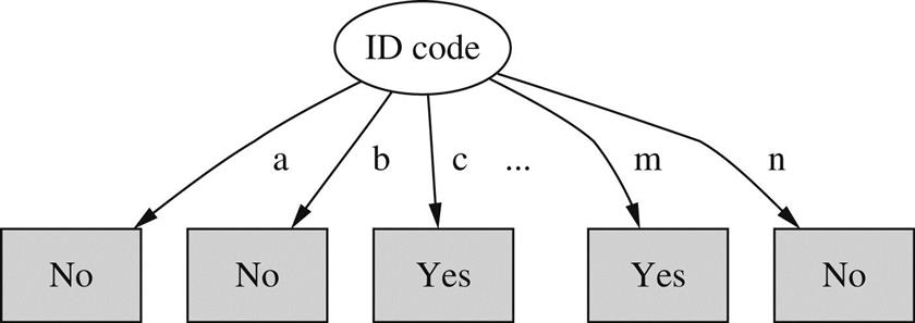
When some attributes have a large number of possible values, giving rise to a multiway branch with many child nodes, a problem arises with the information gain calculation. The problem can best be appreciated in the extreme case when an attribute has a different value for each instance in the dataset—as, e.g., an identification code attribute might.
Table 4.6 gives the weather data with this extra attribute. Branching on ID code produces the tree stump in Fig. 4.5. The expected information required to specify the class given the value of this attribute is
which is zero because each of the 14 terms is zero. This is not surprising: the ID code attribute identifies the instance, which determines the class without any ambiguity—just as Table 4.6 shows. Consequently, the information gain of this attribute is just the information at the root, info([9,5])=0.940 bits. This is greater than the information gain of any other attribute, and so ID code will inevitably be chosen as the splitting attribute. But branching on the identification code is no good for predicting the class of unknown instances.
Table 4.6
The Weather Data with Identification Codes
| ID Code | Outlook | Temperature | Humidity | Windy | Play |
| a | Sunny | Hot | High | False | No |
| b | Sunny | Hot | High | True | No |
| c | Overcast | Hot | High | False | Yes |
| d | Rainy | Mild | High | False | Yes |
| e | Rainy | Cool | Normal | False | Yes |
| f | Rainy | Cool | Normal | True | No |
| g | Overcast | Cool | Normal | True | Yes |
| h | Sunny | Mild | High | False | No |
| i | Sunny | Cool | Normal | False | Yes |
| j | Rainy | Mild | Normal | False | Yes |
| k | Sunny | Mild | Normal | True | Yes |
| l | Overcast | Mild | High | True | Yes |
| m | Overcast | Hot | Normal | False | Yes |
| n | Rainy | Mild | High | True | No |

The overall effect is that the information gain measure tends to prefer attributes with large numbers of possible values. To compensate for this, a modification of the measure called the gain ratio is widely used. The gain ratio is derived by taking into account the number and size of daughter nodes into which an attribute splits the dataset, disregarding any information about the class. In the situation shown in Fig. 4.5, all counts have a value of 1, so the information value of the split is
because the same fraction, 1/14, appears 14 times. This amounts to log 14, or 3.807 bits, which is a very high value. This is because the information value of a split is the number of bits needed to determine to which branch each instance is assigned, and the more branches there are, the greater this value is. The gain ratio is calculated by dividing the original information gain, 0.940 in this case, by the information value of the attribute, 3.807—yielding a gain ratio value of 0.247 for the ID code attribute.
Returning to the tree stumps for the weather data in Fig. 4.2, outlook splits the dataset into three subsets of size 5, 4, and 5 and thus has an intrinsic information value of
without paying any attention to the classes involved in the subsets. As we have seen, this intrinsic information value is greater for a more highly branching attribute such as the hypothesized ID code. Again we can correct the information gain by dividing by the intrinsic information value to get the gain ratio.
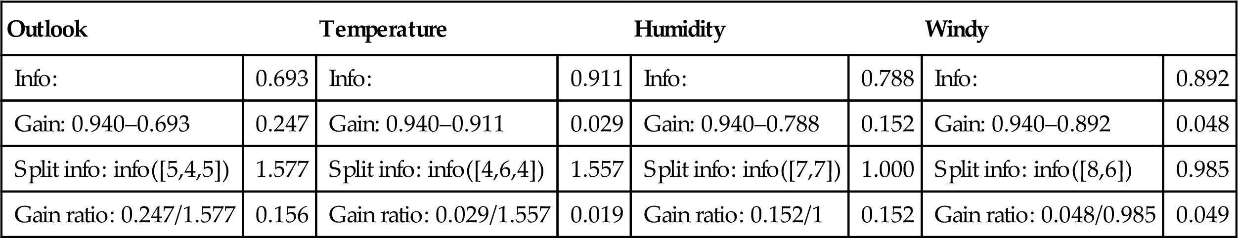
The results of these calculations for the tree stumps of Fig. 4.2 are summarized in Table 4.7 Outlook still comes out on top, but humidity is now a much closer contender because it splits the data into two subsets instead of three. In this particular example, the hypothetical ID code attribute, with a gain ratio of 0.247, would still be preferred to any of these four. However, its advantage is greatly reduced. In practical implementations, we can use an ad hoc test to guard against splitting on such a useless attribute.
Table 4.7
Gain Ratio Calculations for the Tree Stumps of Fig. 4.2
| Outlook | Temperature | Humidity | Windy | ||||
| Info: | 0.693 | Info: | 0.911 | Info: | 0.788 | Info: | 0.892 |
| Gain: 0.940–0.693 | 0.247 | Gain: 0.940–0.911 | 0.029 | Gain: 0.940–0.788 | 0.152 | Gain: 0.940–0.892 | 0.048 |
| Split info: info([5,4,5]) | 1.577 | Split info: info([4,6,4]) | 1.557 | Split info: info([7,7]) | 1.000 | Split info: info([8,6]) | 0.985 |
| Gain ratio: 0.247/1.577 | 0.156 | Gain ratio: 0.029/1.557 | 0.019 | Gain ratio: 0.152/1 | 0.152 | Gain ratio: 0.048/0.985 | 0.049 |
Unfortunately, in some situations the gain ratio modification overcompensates and can lead to preferring an attribute just because its intrinsic information is much lower than for the other attributes. A standard fix is to choose the attribute that maximizes the gain ratio, provided that the information gain for that attribute is at least as great as the average information gain for all the attributes examined.
The basic information-gain algorithm we have described is called ID3. A series of improvements to ID3, including the gain ratio criterion, culminated in a practical and influential system for decision tree induction called C4.5. Further improvements include methods for dealing with numeric attributes, missing values, noisy data, and generating rules from trees, and they are described in Section 6.1.
4.4 Covering Algorithms: Constructing Rules
As we have seen, decision tree algorithms are based on a divide-and-conquer approach to the classification problem. They work top-down, seeking at each stage an attribute to split on that best separates the classes, and then recursively processing the subproblems that result from the split. This strategy generates a decision tree, which can if necessary be converted into a set of classification rules—although if it is to produce effective rules, the conversion is not trivial.
An alternative approach is to take each class in turn and seek a way of covering all instances in it, at the same time excluding instances not in the class. This is called a covering approach because at each stage you identify a rule that “covers” some of the instances. By its very nature, this covering approach leads to a set of rules rather than to a decision tree.
The covering method can readily be visualized in a two-dimensional space of instances as shown in Fig. 4.6A. We first make a rule covering the a’s. For the first test in the rule, split the space vertically as shown in the center picture. This gives the beginnings of a rule:

If x > 1.2 then class = a
However, the rule covers many b’s as well as a’s, so a new test is added to the rule by further splitting the space horizontally as shown in the third diagram:
If x > 1.2 and y > 2.6 then class = a
This gives a rule covering all but one of the a’s. It’s probably appropriate to leave it at that, but if it were felt necessary to cover the final a, another rule would be necessary—perhaps.
If x > 1.4 and y < 2.4 then class = a
The same procedure leads to two rules covering the b’s:
If x ≤1.2 then class = b
If x > 1.2 and y ≤2.6 then class = b
Again, one a is erroneously covered by these rules. If it were necessary to exclude it, more tests would have to be added to the second rule, and additional rules would be needed to cover the b’s that these new tests exclude.
Rules Versus Trees
A top-down divide-and-conquer algorithm operates on the same data in a manner, i.e., at least superficially, quite similar to a covering algorithm. It might first split the dataset using the x attribute, and would probably end up splitting it at the same place, x=1.2. However, whereas the covering algorithm is concerned only with covering a single class, the division would take both classes into account, because divide-and-conquer algorithms create a single concept description that applies to all classes. The second split might also be at the same place, y=2.6, leading to the decision tree in Fig. 4.6B. This tree corresponds exactly to the set of rules, and in this case there is no difference in effect between the covering and the divide-and-conquer algorithms.
But in many situations there is a difference between rules and trees in terms of the perspicuity of the representation. For example, when we described the replicated subtree problem in Section 3.4, we noted that rules can be symmetric whereas trees must select one attribute to split on first, and this can lead to trees that are much larger than an equivalent set of rules. Another difference is that, in the multiclass case, a decision tree split takes all classes into account, trying to maximize the purity of the split, whereas the rule-generating method concentrates on one class at a time, disregarding what happens to the other classes.
A Simple Covering Algorithm
Covering algorithms operate by adding tests to the rule that is under construction, always striving to create a rule with maximum accuracy. In contrast, divide-and-conquer algorithms operate by adding tests to the tree that is under construction, always striving to maximize the separation between the classes. Each of these involves finding an attribute to split on. But the criterion for the best attribute is different in each case. Whereas divide-and-conquer algorithms such as ID3 choose an attribute to maximize the information gain, the covering algorithm we will describe chooses an attribute–value pair to maximize the probability of the desired classification.
Fig. 4.7 gives a picture of the situation, showing the space containing all the instances, a partially constructed rule, and the same rule after a new term has been added. The new term restricts the coverage of the rule: the idea is to include as many instances of the desired class as possible and exclude as many instances of other classes as possible. Suppose the new rule will cover a total of t instances, of which p are positive examples of the class and t–p are in other classes—i.e., they are errors made by the rule. Then choose the new term to maximize the ratio p/t.

An example will help. For a change, we use the contact lens problem of Table 1.1. We will form rules that cover each of the three classes, hard, soft, and none, in turn. To begin, we seek a rule.
If ? then recommendation = hard.
For the unknown term “?,” we have nine choices:
| age = young | 2/8 |
| age = pre-presbyopic | 1/8 |
| age = presbyopic | 1/8 |
| spectacle prescription = myope | 3/12 |
| spectacle prescription = hypermetrope | 1/12 |
| astigmatism = no | 0/12 |
| astigmatism = yes | 4/12 |
| tear production rate = reduced | 0/12 |
| tear production rate = normal | 4/12 |
The numbers on the right show the fraction of “correct” instances in the set singled out by that choice. In this case, correct means that the recommendation is hard. For instance, age=young selects eight instances, two of which recommend hard contact lenses, so the first fraction is 2/8. (To follow this, you will need to look back at the contact lens data in Table 1.1 and count up the entries in the table.) We select the largest fraction, 4/12, arbitrarily choosing between the seventh and the last choice in the list, and create the rule:
If astigmatism = yes then recommendation = hard
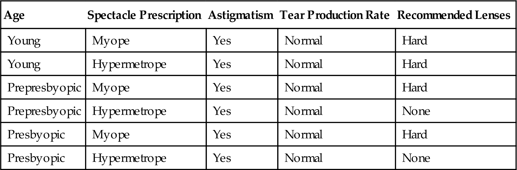
This rule is quite inaccurate, getting only 4 instances correct out of the 12 that it covers, shown in Table 4.8. So we refine it further:
Table 4.8
Part of the Contact Lens Data for which Astigmatism=Yes
| Age | Spectacle Prescription | Astigmatism | Tear Production Rate | Recommended Lenses |
| Young | Myope | Yes | Reduced | None |
| Young | Myope | Yes | Normal | Hard |
| Young | Hypermetrope | Yes | Reduced | None |
| Young | Hypermetrope | Yes | Normal | Hard |
| Prepresbyopic | Myope | Yes | Reduced | None |
| Prepresbyopic | Myope | Yes | Normal | Hard |
| Prepresbyopic | Hypermetrope | Yes | Reduced | None |
| Prepresbyopic | Hypermetrope | Yes | Normal | None |
| Presbyopic | Myope | Yes | Reduced | None |
| Presbyopic | Myope | Yes | Normal | Hard |
| Presbyopic | Hypermetrope | Yes | Reduced | None |
| Presbyopic | Hypermetrope | Yes | Normal | None |

If astigmatism = yes and ? then recommendation = hard
Considering the possibilities for the unknown term ? yields the seven choices:
| age = young | 2/4 |
| age = pre-presbyopic | 1/4 |
| age = presbyopic | 1/4 |
| spectacle prescription = myope | 3/6 |
| spectacle prescription = hypermetrope | 1/6 |
| tear production rate = reduced | 0/6 |
| tear production rate = normal | 4/6 |
(Again, count the entries in Table 4.8.) The last is a clear winner, getting four instances correct out of the six that it covers, and corresponds to the rule.
If astigmatism = yes and tear production rate = normal
then recommendation = hard
Should we stop here? Perhaps. But let’s say we are going for exact rules, no matter how complex they become. Table 4.9 shows the cases that are covered by the rule so far. The possibilities for the next term are now.
| age = young | 2/2 |
| age = pre-presbyopic | 1/2 |
| age = presbyopic | 1/2 |
| spectacle prescription = myope | 3/3 |
| spectacle prescription = hypermetrope | 1/3 |
Table 4.9
Part of the Contact Lens Data for Which Astigmatism=Yes and Tear Production Rate=Normal
| Age | Spectacle Prescription | Astigmatism | Tear Production Rate | Recommended Lenses |
| Young | Myope | Yes | Normal | Hard |
| Young | Hypermetrope | Yes | Normal | Hard |
| Prepresbyopic | Myope | Yes | Normal | Hard |
| Prepresbyopic | Hypermetrope | Yes | Normal | None |
| Presbyopic | Myope | Yes | Normal | Hard |
| Presbyopic | Hypermetrope | Yes | Normal | None |
We need to choose between the first and fourth. So far we have treated the fractions numerically, but although these two are equal (both evaluate to 1), they have different coverage: one selects just two correct instances and the other selects three. In the event of a tie, we choose the rule with the greater coverage, giving the final rule:
If astigmatism = yes and tear production rate = normal
and spectacle prescription = myope then recommendation = hard
This is indeed one of the rules given for the contact lens problem. But it only covers three out of the four hard recommendations. So we delete these three from the set of instances and start again, looking for another rule of the form:
If ? then recommendation = hard
Following the same process, we will eventually find that age=young is the best choice for the first term. Its coverage is one out of seven; the reason for the seven is that 3 instances have been removed from the original set, leaving 21 instances altogether. The best choice for the second term is astigmatism=yes, selecting 1/3 (actually, this is a tie); tear production rate=normal is the best for the third, selecting 1/1.
If age = young and astigmatism = yes
and tear production rate = normal
then recommendation = hard
This rule actually covers two of the original set of instances, one of which is covered by the previous rule—but that’s all right because the recommendation is the same for each rule.
Now that all the hard-lens cases are covered, the next step is to proceed with the soft-lens ones in just the same way. Finally, rules are generated for the none case—unless we are seeking a rule set with a default rule, in which case explicit rules for the final outcome are unnecessary.
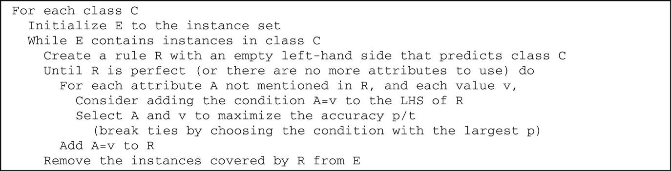
What we have just described is the PRISM method for constructing rules. It generates only correct or “perfect” rules. It measures the success of a rule by the accuracy formula p/t. Any rule with accuracy less than 100% is “incorrect” in that it assigns cases to the class in question that actually do not have that class. PRISM continues adding clauses to each rule until it is perfect: its accuracy is 100%. Fig. 4.8 gives a summary of the algorithm. The outer loop iterates over the classes, generating rules for each class in turn. Note that we reinitialize to the full set of examples each time round. Then we create rules for that class and remove the examples from the set until there are none of that class left. Whenever we create a rule, start with an empty rule (which covers all the examples), and then restrict it by adding tests until it covers only examples of the desired class. At each stage choose the most promising test, i.e., the one that maximizes the accuracy of the rule. Finally, break ties by selecting the test with greatest coverage.
Rules Versus Decision Lists
Consider the rules produced for a particular class, i.e., the algorithm in Fig. 4.8 with the outer loop removed. It seems clear from the way that these rules are produced that they are intended to be interpreted in order, i.e., as a decision list, testing the rules in turn until one applies and then using that. This is because the instances covered by a new rule are removed from the instance set as soon as the rule is completed (in the last line of the code in Fig. 4.8): thus subsequent rules are designed for instances that are not covered by the rule. However, although it appears that we are supposed to check the rules in turn, we do not have to do so. Consider that any subsequent rules generated for this class will have the same effect—they all predict the same class. This means that it does not matter what order they are executed in: either a rule will be found that covers this instance, in which case the class in question is predicted, or no such rule is found, in which case the class is not predicted.
Now return to the overall algorithm. Each class is considered in turn, and rules are generated that distinguish instances in that class from the others. No ordering is implied between the rules for one class and those for another. Consequently the rules that are produced can be executed in any order.
As described in Section 3.4, order-independent rules seem to provide more modularity by acting as independent nuggets of “knowledge,” but they suffer from the disadvantage that it is not clear what to do when conflicting rules apply. With rules generated in this way, a test example may receive multiple classifications, i.e., it may satisfy rules that apply to different classes. Other test examples may receive no classification at all. A simple strategy to force a decision in ambiguous cases is to choose, from the classifications that are predicted, the one with the most training examples or, if no classification is predicted, to choose the category with the most training examples overall. These difficulties do not occur with decision lists because they are meant to be interpreted in order and execution stops as soon as one rule applies: the addition of a default rule at the end ensures that any test instance receives a classification. It is possible to generate good decision lists for the multiclass case using a slightly different method, as we shall see in Section 6.2.
Methods such as Prism can be described as separate-and-conquer algorithms: you identify a rule that covers many instances in the class (and excludes ones not in the class), separate out the covered instances because they are already taken care of by the rule, and continue the process on those that are left. This contrasts with the divide-and-conquer approach of decision trees. The “separate” step results in an efficient method because the instance set continually shrinks as the operation proceeds.
4.5 Mining Association Rules
Association rules are like classification rules. You could find them in the same way, by executing a separate-and-conquer rule-induction procedure for each possible expression that could occur on the right-hand side of the rule. But not only might any attribute occur on the right-hand side with any possible value; a single association rule often predicts the value of more than one attribute. To find such rules, you would have to execute the rule induction procedure once for every possible combination of attributes, with every possible combination of values, on the right-hand side. That would result in an enormous number of association rules, which would then have to be pruned down on the basis of their coverage (the number of instances that they predict correctly) and their accuracy (the same number expressed as a proportion of the number of instances to which the rule applies). This approach is quite infeasible. (Note that, as we mentioned in Section 3.4, what we are calling coverage is often called support and what we are calling accuracy is often called confidence.)
Instead, we capitalize on the fact that we are only interested in association rules with high coverage. We ignore, for the moment, the distinction between the left- and right-hand sides of a rule and seek combinations of attribute–value pairs that have a prespecified minimum coverage. These are called frequent item sets: an attribute–value pair is an item. The terminology derives from market basket analysis, in which the items are articles in your shopping cart and the supermarket manager is looking for associations among these purchases.
Item Sets
The first column of Table 4.10 shows the individual items for the weather data of Table 1.2, with the number of times each item appears in the dataset given at the right. These are the one-item sets. The next step is to generate the two-item sets by making pairs of one-item ones. Of course, there is no point in generating a set containing two different values of the same attribute (such as outlook=sunny and outlook=overcast), because that cannot occur in any actual instance.
Table 4.10
Item Sets for the Weather Data With Coverage 2 or Greater
| One-Item Sets | Two-Item Sets | Three-Item Sets | Four-Item Sets | |||||
| 1 | Outlook=sunny | 5 | Outlook=sunny temperature=mild | 2 | Outlook=sunny temperature=hot humidity=high | 2 | Outlook=sunny temperature=hot humidity=high play=no | 2 |
| 2 | Outlook=overcast | 4 | Outlook=sunny temperature=hot | 2 | Outlook=sunny temperature=hot play=no | 2 | Outlook=sunny humidity=high windy=false play=no | 2 |
| 3 | Outlook=rainy | 5 | Outlook=sunny humidity=normal | 2 | Outlook=sunny humidity=normal play=yes | 2 | Outlook=overcast temperature=hot windy=false play=yes | 2 |
| 4 | Temperature=cool | 4 | Outlook=sunny humidity=high | 3 | Outlook=sunny humidity=high windy=false | 2 | Outlook=rainy temperature=mild windy=false play=yes | 2 |
| 5 | Temperature=mild | 6 | Outlook=sunny windy=true | 2 | Outlook=sunny humidity=high play=no | 3 | Outlook=rainy humidity=normal windy=false play=yes | 2 |
| 6 | Temperature=hot | 4 | Outlook=sunny windy=false | 3 | Outlook=sunny windy=false play=no | 2 | Temperature=cool humidity=normal windy=false play=yes | 2 |
| 7 | Humidity=normal | 7 | Outlook=sunny play=yes | 2 | Outlook=overcast temperature=hot windy=false | 2 | ||
| 8 | Humidity=high | 7 | Outlook=sunny play=no | 3 | Outlook=overcast temperature=hot play=yes | 2 | ||
| 9 | Windy=true | 6 | Outlook=overcast temperature=hot | 2 | Outlook=overcast humidity=normal play=yes | 2 | ||
| 10 | Windy=false | 8 | Outlook=overcast humidity=normal | 2 | Outlook=overcast humidity=high play=yes | 2 | ||
| 11 | Play=yes | 9 | Outlook=overcast humidity=high | 2 | Outlook=overcast windy=true play=yes | 2 | ||
| 12 | Play=no | 5 | Outlook=overcast windy=true | 2 | Outlook=overcast windy=false play=yes | 2 | ||
| 13 | Outlook=overcast windy=false | 2 | Outlook=rainy temperature=cool humidity=normal | 2 | ||||
| … | … | … | ||||||
| 38 | Humidity=normal windy=false | 4 | Humidity=normal windy=false play=yes | 4 | ||||
| 39 | Humidity=normal play=yes | 6 | Humidity=high windy=false play=no | 2 | ||||
| 40 | Humidity=high windy=true | 3 | ||||||
| … | … | |||||||
| 47 | Windy=false play=no | 2 |
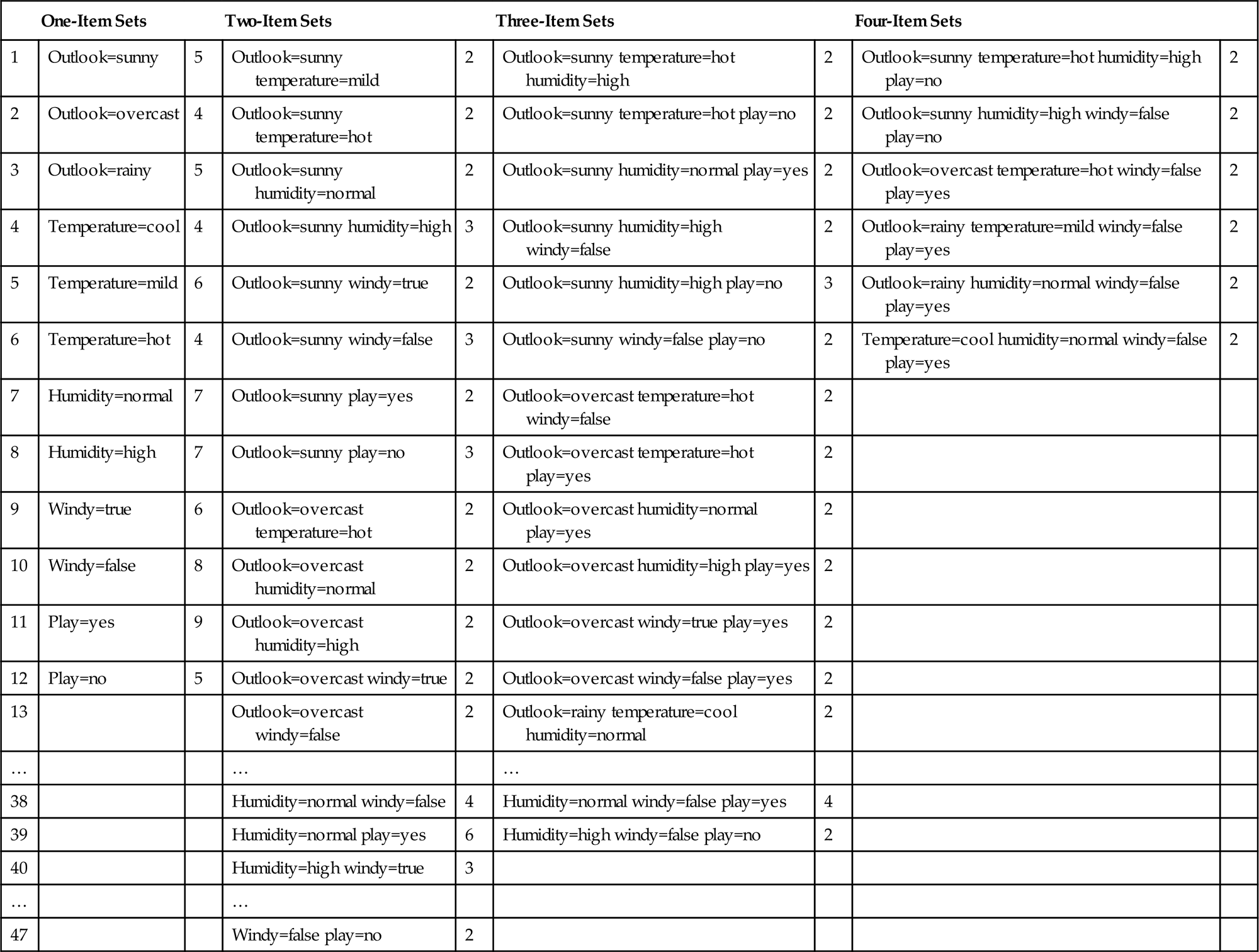
Assume that we seek association rules with minimum coverage 2: thus we discard any item sets that cover fewer than two instances. This leaves 47 two-item sets, some of which are shown in the second column along with the number of times they appear. The next step is to generate the three-item sets, of which 39 have a coverage of 2 or greater. There are 6 four-item sets, and no five-item sets—for this data, a five-item set with coverage 2 or greater could only correspond to a repeated instance. The first rows of the table, e.g., show that there are 5 days when outlook=sunny, two of which have temperature=hot, and, in fact, on both of those days humidity=high and play=no as well.
Association Rules
Shortly we will explain how to generate these item sets efficiently. But first let us finish the story. Once all item sets with the required coverage have been generated, the next step is to turn each into a rule, or set of rules, with at least the specified minimum accuracy. Some item sets will produce more than one rule; others will produce none. For example, there is one three-item set with a coverage of 4 (row 38 of Table 4.10):
humidity = normal, windy = false, play = yes
This set leads to seven potential rules:
| If humidity = normal and windy = false then play = yes | 4/4 |
| If humidity = normal and play = yes then windy = false | 4/6 |
| If windy = false and play = yes then humidity = normal | 4/6 |
| If humidity = normal then windy = false and play = yes | 4/7 |
| If windy = false then humidity = normal and play = yes | 4/8 |
| If play = yes then humidity = normal and windy = false | 4/9 |
| If–then humidity = normal and windy = false and play = yes | 4/14 |
The figures at the right show the number of instances for which all three conditions are true—i.e., the coverage—divided by the number of instances for which the conditions in the antecedent are true. Interpreted as a fraction, they represent the proportion of instances on which the rule is correct—i.e., its accuracy. Assuming that the minimum specified accuracy is 100%, only the first of these rules will make it into the final rule set. The denominators of the fractions are readily obtained by looking up the antecedent expression in Table 4.10 (although some are not shown in the table). The final rule above has no conditions in the antecedent, and its denominator is the total number of instances in the dataset.
Table 4.11 shows the final rule set for the weather data, with minimum coverage 2 and minimum accuracy 100%, sorted by coverage. There are 58 rules, 3 with coverage 4, 5 with coverage 3, and 50 with coverage 2. Only 7 have two conditions in the consequent, and none has more than two. The first rule comes from the item set described previously. Sometimes several rules arise from the same item set. For example, rules 9, 10, and 11 all arise from the four-item set in row 6 of Table 4.10:
Table 4.11
Association Rules for the Weather Data
| Association Rule | Coverage | Accuracy (%) | |||
| 1 | Humidity=normal windy=false | ⇒ | Play=yes | 4 | 100 |
| 2 | Temperature=cool | ⇒ | Humidity=normal | 4 | 100 |
| 3 | Outlook=overcast | ⇒ | Play=yes | 4 | 100 |
| 4 | Temperature=cool play=yes | ⇒ | Humidity=normal | 3 | 100 |
| 5 | Outlook=rainy windy=false | ⇒ | Play=yes | 3 | 100 |
| 6 | Outlook=rainy play=yes | ⇒ | Windy=false | 3 | 100 |
| 7 | Outlook=sunny humidity=high | ⇒ | Play=no | 3 | 100 |
| 8 | Outlook=sunny play=no | ⇒ | Humidity=high | 3 | 100 |
| 9 | Temperature=cool windy=false | ⇒ | Humidity=normal play=yes | 2 | 100 |
| 10 | Temperature=cool humidity=normal windy=false⇒ | ⇒ | Play=yes | 2 | 100 |
| 11 | Temperature=cool windy=false play=yes | ⇒ | Humidity=normal | 2 | 100 |
| 12 | Outlook=rainy humidity=normal windy=false | ⇒ | Play=yes | 2 | 100 |
| 13 | Outlook=rainy humidity=normal play=yes | ⇒ | Windy=false | 2 | 100 |
| 14 | Outlook=rainy temperature=mild windy=false | ⇒ | Play=yes | 2 | 100 |
| 15 | Outlook=rainy temperature=mild play=yes | ⇒ | Windy=false | 2 | 100 |
| 16 | Temperature=mild windy=false play=yes | ⇒ | Outlook=rainy | 2 | 100 |
| 17 | Outlook=overcast temperature=hot | ⇒ | Windy=false play=yes | 2 | 100 |
| 18 | Outlook=overcast windy=false | ⇒ | Temperature=hot play=yes | 2 | 100 |
| 19 | Temperature=hot play=yes | ⇒ | Outlook=overcast windy=false | 2 | 100 |
| 20 | Outlook=overcast temperature=hot windy=false ⇒ | ⇒ | Play=yes | 2 | 100 |
| 21 | Outlook=overcast temperature=hot play=yes | ⇒ | Windy=false | 2 | 100 |
| 22 | Outlook=overcast windy=false play=yes | ⇒ | Temperature=hot | 2 | 100 |
| 23 | Temperature=hot windy=false play=yes | ⇒ | Outlook=overcast | 2 | 100 |
| 24 | Windy=false play=no | ⇒ | Outlook=sunny humidity=high | 2 | 100 |
| 25 | Outlook=sunny humidity=high windy=false | ⇒ | Play=no | 2 | 100 |
| 26 | Outlook=sunny windy=false play=no | ⇒ | Humidity=high | 2 | 100 |
| 27 | Humidity=high windy=false play=no | ⇒ | Outlook=sunny | 2 | 100 |
| 28 | Outlook=sunny temperature=hot | ⇒ | Humidity=high play=no | 2 | 100 |
| 29 | Temperature=hot play=no | ⇒ | Outlook=sunny humidity=high | 2 | 100 |
| 30 | Outlook=sunny temperature=hot humidity=high | ⇒ | Play=no | 2 | 100 |
| 31 | Outlook=sunny temperature=hot play=no | ⇒ | Humidity=high | 2 | 100 |
| … | … | … | … | ||
| 58 | Outlook=sunny temperature=hot | ⇒ | Humidity=high | 2 | 100 |

temperature = cool, humidity = normal, windy = false, play = yes
which has coverage 2. Three subsets of this item set also have coverage 2:
temperature = cool, windy = false
temperature = cool, humidity = normal, windy = false
temperature = cool, windy = false, play = yes
and these lead to rules 9, 10, and 11, all of which are 100% accurate (on the training data).
Generating Rules Efficiently
We now consider in more detail an algorithm for producing association rules with specified minimum coverage and accuracy. There are two stages: generating item sets with the specified minimum coverage, and from each item set determining the rules that have the specified minimum accuracy.
The first stage proceeds by generating all one-item sets with the given minimum coverage (the first column of Table 4.10) and then using this to generate the two-item sets (second column), three-item sets (third column), and so on. Each operation involves a pass through the dataset to count the items in each set, and after the pass the surviving item sets are stored in a hash table—a standard data structure that allows elements stored in it to be found very quickly. From the one-item sets, candidate two-item sets are generated, and then a pass is made through the dataset, counting the coverage of each two-item set; at the end the candidate sets with less than minimum coverage are removed from the table. The candidate two-item sets are simply all of the one-item sets taken in pairs, because a two-item set cannot have the minimum coverage unless both its constituent one-item sets have the minimum coverage, too. This applies in general: a three-item set can only have the minimum coverage if all three of its two-item subsets have minimum coverage as well, and similarly for four-item sets.
An example will help to explain how candidate item sets are generated. Suppose there are five three-item sets: (A B C), (A B D), (A C D), (A C E), and (B C D)—where, e.g., A is a feature such as outlook=sunny. The union of the first two, (A B C D), is a candidate four-item set because its other three-item subsets (A C D) and (B C D) have greater than minimum coverage. If the three-item sets are sorted into lexical order, as they are in this list, then we need only consider pairs whose first two members are the same. For example, we do not consider (A C D) and (B C D) because (A B C D) can also be generated from (A B C) and (A B D), and if these two are not three-item sets with minimum coverage then (A B C D) cannot be a candidate four-item set. This leaves the pairs (A B C) and (A B D), which we have already explained, and (A C D) and (A C E). This second pair leads to the set (A C D E) whose three-item subsets do not all have the minimum coverage, so it is discarded. The hash table assists with this check: we simply remove each item from the set in turn and check that the remaining three-item set is indeed present in the hash table. Thus in this example there is only one candidate four-item set, (A B C D). Whether or not it actually has minimum coverage can only be determined by checking the instances in the dataset.
The second stage of the procedure takes each item set and generates rules from it, checking that they have the specified minimum accuracy. If only rules with a single test on the right-hand side were sought, it would be simply a matter of considering each condition in turn as the consequent of the rule, deleting it from the item set, and dividing the coverage of the entire item set by the coverage of the resulting subset—obtained from the hash table—to yield the accuracy of the corresponding rule. Given that we are also interested in association rules with multiple tests in the consequent, it looks like we have to evaluate the effect of placing each subset of the item set on the right-hand side, leaving the remainder of the set as the antecedent.
This brute-force method will be excessively computation intensive unless item sets are small, because the number of possible subsets grows exponentially with the size of the item set. However, there is a better way. We observed when describing association rules in Section 3.4 that if the double-consequent rule
If windy = false and play = no
then outlook = sunny and humidity = high
holds with a given minimum coverage and accuracy, then both single-consequent rules formed from the same item set must also hold:
If humidity = high and windy = false and play = no
then outlook = sunny
If outlook = sunny and windy = false and play = no
then humidity = high
Conversely, if one or other of the single-consequent rules does not hold, there is no point in considering the double-consequent one. This gives a way of building up from single-consequent rules to candidate double-consequent ones, from double-consequent rules to candidate triple-consequent ones, and so on. Of course, each candidate rule must be checked against the hash table to see if it really does have more than the specified minimum accuracy. But this generally involves checking far fewer rules than the brute force method. It is interesting that this way of building up candidate (n+1)-consequent rules from actual n-consequent ones is really just the same as building up candidate (n+1)-item sets from actual n-item sets, described earlier.
Fig. 4.9 shows pseudocode for the two parts of the association rule mining process. Fig. 4.9A shows how to find all item sets of sufficient coverage. In an actual implementation, the minimum coverage (or support) would be specified by a parameter whose value the user can specify. Fig. 4.9B shows how to find all rules that are sufficiently accurate, for a particular item set found by the previous algorithm. Again, in practice, minimum accuracy (or confidence) would be determined by a user-specified parameter.

To find all rules for a particular dataset, the process shown in the second part would be applied to all the item sets found using the algorithm in the first part. Note that the code in the second part requires access to the hash tables established by the first part, which contain all the sufficiently frequent item sets that have been found, along with their coverage. In this manner, the algorithm in Fig. 4.9B does not need to revisit the original data at all: accuracy can be estimated based on the information in these tables.
Association rules are often sought for very large datasets, and efficient algorithms are highly valued. The method we have described makes one pass through the dataset for each different size of item set. Sometimes the dataset is too large to read in to main memory and must be kept on disk; then it may be worth reducing the number of passes by checking item sets of two consecutive sizes in one go. For example, once sets with two items have been generated, all sets of three items could be generated from them before going through the instance set to count the actual number of items in the sets. More three-item sets than necessary would be considered, but the number of passes through the entire dataset would be reduced.
In practice, the amount of computation needed to generate association rules depends critically on the minimum coverage specified. The accuracy has less influence because it does not affect the number of passes that must be made through the dataset. In many situations we would like to obtain a certain number of rules—say 50—with the greatest possible coverage at a prespecified minimum accuracy level. One way to do this is to begin by specifying the coverage to be rather high and to then successively reduce it, reexecuting the entire rule-finding algorithm for each coverage value and repeating until the desired number of rules has been generated.
The tabular input format that we use throughout this book, and in particular the standard ARFF format based on it, is very inefficient for many association-rule problems. Association rules are often used in situations where attributes are binary—either present or absent—and most of the attribute values associated with a given instance are absent. This is a case for the sparse data representation described in Section 2.4; the same algorithm for finding association rules applies.
4.6 Linear Models
The methods we have been looking at for decision trees and rules work most naturally with nominal attributes. They can be extended to numeric attributes either by incorporating numeric-value tests directly into the decision tree or rule induction scheme, or by prediscretizing numeric attributes into nominal ones. We will see how in Chapter 6, Trees and rules, and Chapter 8, Data transformations. However, there are methods that work most naturally with numeric attributes, namely, the linear models introduced in Section 3.2; we examine them in more detail here. They can form components or starting points for more complex learning methods, which we will investigate later.
Numeric Prediction: Linear Regression
When the outcome, or class, is numeric, and all the attributes are numeric, linear regression is a natural technique to consider. This is a staple method in statistics. The idea is to express the class as a linear combination of the attributes, with predetermined weights:
where x is the class; a1, a2,…, ak are the attribute values; and w0, w1,…, wk are weights.
The weights are calculated from the training data. Here the notation gets a little heavy, because we need a way of expressing the attribute values for each training instance. The first instance will have a class, say x(1), and attribute values, ![]() ,
, ![]() ,…,
,…, ![]() , where the superscript denotes that it is the first example. Moreover, it is notationally convenient to assume an extra attribute a0, whose value is always 1.
, where the superscript denotes that it is the first example. Moreover, it is notationally convenient to assume an extra attribute a0, whose value is always 1.
The predicted value for the first instance’s class can be written as
This is the predicted, not the actual, value for the class. Of interest is the difference between the predicted and actual values. The method of least-squares linear regression is to choose the coefficients wj—there are k+1 of them—to minimize the sum of the squares of these differences over all the training instances. Suppose there are n training instances: denote the ith one with a superscript (i). Then the sum of the squares of the differences is
where the expression inside the parentheses is the difference between the ith instance’s actual class and its predicted class. This sum of squares is what we have to minimize by choosing the coefficients appropriately.
This is all starting to look rather formidable. However, the minimization technique is straightforward if you have the appropriate math background. Suffice it to say that given enough examples—roughly speaking, more examples than attributes—choosing weights to minimize the sum of the squared differences is really not difficult. It does involve a matrix inversion operation, but this is readily available as prepackaged software.
Once the math has been accomplished, the result is a set of numeric weights, based on the training data, which can be used to predict the class of new instances. We saw an example of this when looking at the CPU performance data, and the actual numeric weights are given in Fig. 3.4A. This formula can be used to predict the CPU performance of new test instances.
Linear regression is an excellent, simple method for numeric prediction, and it has been widely used in statistical applications for decades. Of course, basic linear models suffer from the disadvantage of, well, linearity. If the data exhibits a nonlinear dependency, the best-fitting straight line will be found, where “best” is interpreted as the least mean-squared difference. This line may not fit very well. However, linear models serve well as building blocks or starting points for more complex learning methods.
Linear Classification: Logistic Regression
Linear regression can easily be used for classification in domains with numeric attributes. Indeed, we can use any regression technique for classification. The trick is to perform a regression for each class, setting the output equal to one for training instances that belong to the class and zero for those that do not. The result is a linear expression for the class. Then, given a test example of unknown class, calculate the value of each linear expression and choose the one that is largest. When used with linear regression, this scheme is sometimes called multiresponse linear regression.
One way of looking at multiresponse linear regression is to imagine that it approximates a numeric membership function for each class. The membership function is 1 for instances that belong to that class and 0 for other instances. Given a new instance we calculate its membership for each class and select the biggest.
Multiresponse linear regression often yields good results in practice. However, it has two drawbacks. First, the membership values it produces are not proper probabilities because they can fall outside the range 0–1. Second, least-squares regression assumes that the errors are not only statistically independent, but are also normally distributed with the same standard deviation, an assumption that is blatantly violated when the method is applied to classification problems because the observations only ever take on the values 0 and 1.
A related statistical technique called logistic regression does not suffer from these problems. Instead of approximating the 0 and 1 values directly, thereby risking illegitimate probability values when the target is overshot, logistic regression builds a linear model based on a transformed target variable.
Suppose first that there are only two classes. Logistic regression replaces the original target variable
which cannot be approximated accurately using a linear function, by
The resulting values are no longer constrained to the interval from 0 to 1 but can lie anywhere between negative infinity and positive infinity. Fig. 4.10A plots the transformation function, which is often called the logit transformation.

The transformed variable is approximated using a linear function just like the ones generated by linear regression. The resulting model is
with weights w. Fig. 4.10B shows an example of this function in one dimension, with two weights w0=−1.25 and w1=0.5.
Just as in linear regression, weights must be found that fit the training data well. Linear regression measures goodness of fit using the squared error. In logistic regression the log-likelihood of the model is used instead. This is given by
where the x(i) are either zero or one.
The weights wi need to be chosen to maximize the log-likelihood. There are several methods for solving this maximization problem. A simple one is to iteratively solve a sequence of weighted least-squares regression problems until the log-likelihood converges to a maximum, which usually happens in a few iterations.
To generalize logistic regression to several classes, one possibility is to proceed in the way described above for multiresponse linear regression by performing logistic regression independently for each class. Unfortunately, the resulting probability estimates will not generally sum to one. To obtain proper probabilities it is necessary to couple the individual models for each class. This yields a joint optimization problem, and there are efficient solution methods for this.
The use of linear functions for classification can easily be visualized in instance space. The decision boundary for two-class logistic regression lies where the prediction probability is 0.5, i.e.:
This occurs when
Because this is a linear equality in the attribute values, the boundary is a plane, or hyperplane, in instance space. It is easy to visualize sets of points that cannot be separated by a single hyperplane, and these cannot be discriminated correctly by logistic regression.
Multiresponse linear regression suffers from the same problem. Each class receives a weight vector calculated from the training data. Focus for the moment on a particular pair of classes. Suppose the weight vector for class 1 is
and the same for class 2 with appropriate superscripts. Then, an instance will be assigned to class 1 rather than class 2 if
In other words, it will be assigned to class 1 if
This is a linear inequality in the attribute values, so the boundary between each pair of classes is a hyperplane.
Linear Classification Using the Perceptron
Logistic regression attempts to produce accurate probability estimates by maximizing the probability of the training data. Of course, accurate probability estimates lead to accurate classifications. However, it is not necessary to perform probability estimation if the sole purpose of the model is to predict class labels. A different approach is to learn a hyperplane that separates the instances pertaining to the different classes—let’s assume that there are only two of them. If the data can be separated perfectly into two groups using a hyperplane, it is said to be linearly separable. It turns out that if the data is linearly separable, there is a very simple algorithm for finding a separating hyperplane.
The algorithm is called the perceptron learning rule. Before looking at it in detail, let’s examine the equation for a hyperplane again:
Here, a1, a2,…, ak are the attribute values, and w0, w1,…, wk are the weights that define the hyperplane. We will assume that each training instance a1, a2,… is extended by an additional attribute a0 that always has the value 1 (as we did in the case of linear regression). This extension, which is called the bias, just means that we don’t have to include an additional constant element in the sum. If the sum is greater than zero, we will predict the first class; otherwise, we will predict the second class. We want to find values for the weights so that the training data is correctly classified by the hyperplane.
Fig. 4.11A gives the perceptron learning rule for finding a separating hyperplane. The algorithm iterates until a perfect solution has been found, but it will only work properly if a separating hyperplane exists, i.e., if the data is linearly separable. Each iteration goes through all the training instances. If a misclassified instance is encountered, the parameters of the hyperplane are changed so that the misclassified instance moves closer to the hyperplane or maybe even across the hyperplane onto the correct side. If the instance belongs to the first class, this is done by adding its attribute values to the weight vector; otherwise, they are subtracted from it.

To see why this works, consider the situation after an instance a pertaining to the first class has been added:
This means the output for a has increased by
This number is always positive. Thus the hyperplane has moved in the correct direction for classifying instance a as positive. Conversely, if an instance belonging to the second class is misclassified, the output for that instance decreases after the modification, again moving the hyperplane in the correct direction.
These corrections are incremental, and can interfere with earlier updates. However, it can be shown that the algorithm converges into a finite number of iterations if the data is linearly separable. Of course, if the data is not linearly separable, the algorithm will not terminate, so an upper bound needs to be imposed on the number of iterations when this method is applied in practice.
The resulting hyperplane is called a perceptron, and it’s the grandfather of neural networks (we return to neural networks in Section 7.2 and chapter: Deep learning). Fig. 4.11B represents the perceptron as a graph with nodes and weighted edges, imaginatively termed a “network” of “neurons.” There are two layers of nodes: input and output. The input layer has one node for every attribute, plus an extra node that is always set to one. The output layer consists of just one node. Every node in the input layer is connected to the output layer. The connections are weighted, and the weights are those numbers found by the perceptron learning rule.
When an instance is presented to the perceptron, its attribute values serve to “activate” the input layer. They are multiplied by the weights and summed up at the output node. If the weighted sum is greater than 0 the output signal is 1, representing the first class; otherwise, it is −1, representing the second.
Linear Classification Using Winnow
The perceptron algorithm is not the only method that is guaranteed to find a separating hyperplane for a linearly separable problem. For datasets with binary attributes there is an alternative known as Winnow, shown in Fig. 4.12A. The structure of the two algorithms is very similar. Like the perceptron, Winnow only updates the weight vector when a misclassified instance is encountered—it is mistake driven.
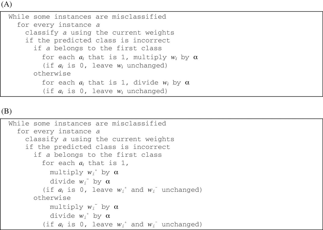
The two methods differ in how the weights are updated. The perceptron rule employs an additive mechanism that alters the weight vector by adding (or subtracting) the instance’s attribute vector. Winnow employs multiplicative updates and alters weights individually by multiplying them by a user-specified parameter α (or its inverse). The attribute values ai are either 0 or 1 because we are working with binary data. Weights are unchanged if the attribute value is 0, because then they do not participate in the decision. Otherwise, the multiplier is α if that attribute helps to make a correct decision and 1/α if it does not.
Another difference is that the threshold in the linear function is also a user-specified parameter. We call this threshold θ and classify an instance as belonging to class 1 if and only if
The multiplier α needs to be greater than one. The wi are set to a constant at the start.
The algorithm we have described doesn’t allow for negative weights, which—depending on the domain—can be a drawback. However, there is a version, called Balanced Winnow, which does allow them. This version maintains two weight vectors, one for each class. An instance is classified as belonging to class 1 if:
Fig. 4.12B shows the balanced algorithm.
Winnow is very effective in homing in on the relevant features in a dataset—therefore it is called an attribute-efficient learner. That means that it may be a good candidate algorithm if a dataset has many (binary) features and most of them are irrelevant. Both Winnow and the perceptron algorithm can be used in an online setting in which new instances arrive continuously, because they can incrementally update their concept descriptions as new instances arrive.
4.7 Instance-Based Learning
In instance-based learning the training examples are stored verbatim, and a distance function is used to determine which member of the training set is closest to an unknown test instance. Once the nearest training instance has been located, its class is predicted for the test instance. The only remaining problem is defining the distance function, and that is not very difficult to do, particularly if the attributes are numeric.
The Distance Function
Although there are other possible choices, most instance-based learners use Euclidean distance. The distance between an instance with attribute values ![]() ,
, ![]() ,…,
,…, ![]() (where k is the number of attributes) and one with values
(where k is the number of attributes) and one with values ![]() ,
, ![]() ,…,
,…, ![]() is defined as
is defined as
When comparing distances it is not necessary to perform the square root operation: the sums of squares can be compared directly. One alternative to the Euclidean distance is the Manhattan or city-block metric, where the difference between attribute values is not squared but just added up (after taking the absolute value). Others are obtained by taking powers higher than the square. Higher powers increase the influence of large differences at the expense of small differences. Generally, the Euclidean distance represents a good compromise. Other distance metrics may be more appropriate in special circumstances. The key is to think of actual instances and what it means for them to be separated by a certain distance—What would twice that distance mean, for example?
Different attributes are measured on different scales, so if the Euclidean distance formula were used directly, the effect of some attributes might be completely dwarfed by others that had larger scales of measurement. Consequently, it is usual to normalize all attribute values to lie between 0 and 1, by calculating
where vi is the actual value of attribute i, and the maximum and minimum are taken over all instances in the training set.
These formulae implicitly assume numeric attributes. Here the difference between two values is just the numerical difference between them, and it is this difference that is squared and added to yield the distance function. For nominal attributes that take on values that are symbolic rather than numeric, the difference between two values that are not the same is often taken to be one, whereas if the values are the same the difference is zero. No scaling is required in this case because only the values 0 and 1 are used.
A common policy for handling missing values is as follows: for nominal attributes, assume that a missing feature is maximally different from any other feature value. Thus if either or both values are missing, or if the values are different, the difference between them is taken as one; the difference is zero only if they are not missing and both are the same. For numeric attributes, the difference between two missing values is also taken as one. However, if just one value is missing, the difference is often taken as either the (normalized) size of the other value or one minus that size, whichever is larger. This means that if values are missing, the difference is as large as it can possibly be.
Finding Nearest Neighbors Efficiently
Although instance-based learning is simple and effective, it is often slow. The obvious way to find which member of the training set is closest to an unknown test instance is to calculate the distance from every member of the training set and select the smallest. This procedure is linear in the number of training instances: in other words, the time it takes to make a single prediction is proportional to the number of training instances. Processing an entire test set takes time proportional to the product of the number of instances in the training and test sets.
Nearest neighbors can be found more efficiently by representing the training set as a tree, although it is not quite obvious how. One suitable structure is a kD-tree. This is a binary tree that divides the input space with a hyperplane and then splits each partition again, recursively. All splits are made parallel to one of the axes, either vertically or horizontally, in the two-dimensional case. The data structure is called a kD-tree because it stores a set of points in k-dimensional space, k being the number of attributes.
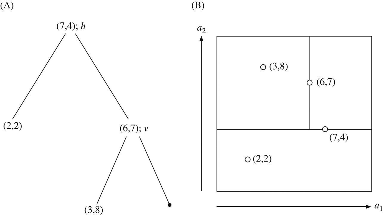
Fig. 4.13A gives a small example with k=2, and Fig. 4.13B shows the four training instances it represents, along with the hyperplanes that constitute the tree. Note that these hyperplanes are not decision boundaries: decisions are made on a nearest-neighbor basis as explained later. The first split is horizontal (h), through the point (7,4)—this is the tree’s root. The left branch is not split further: it contains the single point (2,2), which is a leaf of the tree. The right branch is split vertically (v) at the point (6,7). Its right child is empty, and its left child contains the point (3,8). As this example illustrates, each region contains just one point—or, perhaps, no points. Sibling branches of the tree—e.g., the two daughters of the root in Fig. 4.13A—are not necessarily developed to the same depth. Every point in the training set corresponds to a single node, and up to half are leaf nodes.
How do you build a kD-tree from a dataset? Can it be updated efficiently as new training examples are added? And how does it speed up nearest-neighbor calculations? We tackle the last question first.
To locate the nearest neighbor of a given target point, follow the tree down from its root to locate the region containing the target. Fig. 4.14 shows a space like that of Fig. 4.13B but with a few more instances and an extra boundary. The target, which is not one of the instances in the tree, is marked by a star. The leaf node of the region containing the target is colored black. This is not necessarily the target’s closest neighbor, as this example illustrates, but it is a good first approximation. In particular, any nearer neighbor must lie closer—within the dashed circle in Fig. 4.14. To determine whether one exists, first check whether it is possible for a closer neighbor to lie within the node’s sibling. The black node’s sibling is shaded in Fig. 4.14, and the circle does not intersect it, so the sibling cannot contain a closer neighbor. Then back up to the parent node and check its sibling—which here covers everything above the horizontal line. In this case it must to be explored, because the area it covers intersects with the best circle so far. To explore it, find its daughters (the original point’s two aunts), check whether they intersect the circle (the left one does not, but the right one does), and descend to see if it contains a closer point (it does).

In a typical case, this algorithm is far faster than examining all points to find the nearest neighbor. The work involved in finding the initial approximate nearest neighbor—the black point in Fig. 4.14—depends on the depth of the tree, given by the logarithm log2n of the number of nodes n, if the tree is well balanced. The amount of work involved in backtracking to check whether this really is the nearest neighbor depends a bit on the tree, and on how good the initial approximation is. But for a well-constructed tree whose nodes are approximately square, rather than long skinny rectangles, it can also be shown to be logarithmic in the number of nodes (if the number of attributes in the dataset is not too large).
How do you build a good tree for a set of training examples? The problem boils down to selecting the first training instance to split at and the direction of the split. Once you can do that, apply the same method recursively to each child of the initial split to construct the entire tree.
To find a good direction for the split, calculate the variance of the data points along each axis individually, select the axis with the greatest variance, and create a splitting hyperplane perpendicular to it. To find a good place for the hyperplane, locate the median value along that axis and select the corresponding point. This makes the split perpendicular to the direction of greatest spread, with half the points lying on either side. This produces a well-balanced tree. To avoid long skinny regions it is best for successive splits to be along different axes, which is likely because the dimension of greatest variance is chosen at each stage. However, if the distribution of points is badly skewed, choosing the median value may generate several successive splits in the same direction, yielding long, skinny hyperrectangles. A better strategy is to calculate the mean rather than the median and use the point closest to that. The tree will not be perfectly balanced, but its regions will tend to be squarish because there is a greater chance that different directions will be chosen for successive splits.
An advantage of instance-based learning over most other machine learning methods is that new examples can be added to the training set at any time. To retain this advantage when using a kD-tree, we need to be able to update it incrementally with new data points. To do this, determine which leaf node contains the new point and find its hyperrectangle. If it is empty, simply place the new point there. Otherwise split the hyperrectangle, splitting it along its longest dimension to preserve squareness. This simple heuristic does not guarantee that adding a series of points will preserve the tree’s balance, nor that the hyperrectangles will be well shaped for nearest-neighbor search. It is a good idea to rebuild the tree from scratch occasionally—e.g., when its depth grows to twice the best possible depth.
As we have seen, kD-trees are good data structures for finding nearest neighbors efficiently. However, they are not perfect. Skewed datasets present a basic conflict between the desire for the tree to be perfectly balanced and the desire for regions to be squarish. More importantly, rectangles—even squares—are not the best shape to use anyway, because of their corners. If the dashed circle in Fig. 4.14 were any bigger, which it would be if the black instance were a little further from the target, it would intersect the lower right-hand corner of the rectangle at the top left and then that rectangle would have to be investigated, too—despite the fact that the training instances that define it are a long way from the corner in question. The corners of rectangular regions are awkward.
The solution? Use hyperspheres, not hyperrectangles. Neighboring spheres may overlap whereas rectangles can abut, but this is not a problem because the nearest-neighbor algorithm for kD-trees does not depend on the regions being disjoint. A data structure called a ball tree defines k-dimensional hyperspheres (balls) that cover the data points, and arranges them into a tree.
Fig. 4.15A shows 16 training instances in two-dimensional space, overlaid by a pattern of overlapping circles, and Fig. 4.15B shows a tree formed from these circles. Circles at different levels of the tree are indicated by different styles of dash, and the smaller circles are drawn in shades of gray. Each node of the tree represents a ball, and the node is dashed or shaded according to the same convention so that you can identify which level the balls are at. To help you understand the tree, numbers are placed on the nodes to show how many data points are deemed to be inside that ball. But be careful: this is not necessarily the same as the number of points falling within the spatial region that the ball represents. The regions at each level sometimes overlap, but points that fall into the overlap area are assigned to only one of the overlapping balls (the diagram does not show which one). Instead of the occupancy counts in Fig. 4.15B the nodes of actual ball trees store the center and radius of their ball; leaf nodes record the points they contain as well.

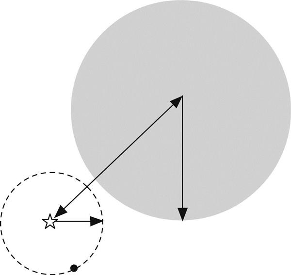
To use a ball tree to find the nearest neighbor to a given target, start by traversing the tree from the top down to locate the leaf that contains the target and find the closest point to the target in that ball. (If no ball contains the instance, pick the closest ball.) This gives an upper bound for the target’s distance from its nearest neighbor. Then, just as for the kD-tree, examine the sibling node. If the distance from the target to the sibling’s center exceeds its radius plus the current upper bound, it cannot possibly contain a closer point; otherwise the sibling must be examined by descending the tree further. In Fig. 4.16 the target is marked with a star and the black dot is its closest currently known neighbor. The entire contents of the gray ball can be ruled out: it cannot contain a closer point because its center is too far away. Proceed recursively back up the tree to its root, examining any ball that may possibly contain a point nearer than the current upper bound.
Ball trees are built from the top down, and as with kD-trees the basic problem is to find a good way of splitting a ball containing a set of data points into two. In practice you do not have to continue until the leaf balls contain just two points: you can stop earlier, once a predetermined minimum number is reached—and the same goes for kD-trees. Here is one possible splitting method. Choose the point in the ball that is farthest from its center, and then a second point that is farthest from the first one. Assign all data points in the ball to the closest one of these two provisional cluster centers, then compute the centroid of each cluster and the minimum radius required for it to enclose all the data points it represents. This method has the merit that the cost of splitting a ball containing n points is only linear in n. There are more elaborate algorithms that produce tighter balls, but they require more computation. We will not describe sophisticated algorithms for constructing ball trees or updating them incrementally as new training instances are encountered.
Remarks
Nearest-neighbor instance-based learning is simple and often works very well. In the scheme we have described each attribute has exactly the same influence on the decision, just as it does in the Naïve Bayes method. Another problem is that the database can easily become corrupted by noisy exemplars. One solution is to adopt the k-nearest neighbor strategy, where some fixed, small, number k of nearest neighbors—say five—are located and used together to determine the class of the test instance through a simple majority vote. (Note that earlier we used k to denote the number of attributes; this is a different, independent usage.) Another way of proofing the database against noise is to choose the exemplars that are added to it selectively and judiciously. Improved procedures, described in Section 7.1, address these shortcomings.
The nearest-neighbor method originated many decades ago, and statisticians analyzed k-nearest-neighbor schemes in the early 1950s. If the number of training instances is large, it makes intuitive sense to use more than one nearest neighbor, but clearly this is dangerous if there are few instances. It can be shown that when k and the number n of instances both become infinite in such a way that k/n→0, the probability of error approaches the theoretical minimum for the dataset. The nearest-neighbor method was adopted as a classification scheme in the early 1960s and has been widely used in the field of pattern recognition for almost half a century.
Nearest-neighbor classification was notoriously slow until kD-trees began to be applied in the early 1990s, although the data structure itself was developed much earlier. In practice, these trees become inefficient when the dimension of the space increases and are only worthwhile when the number of attributes is relatively small. Ball trees were developed much more recently and are an instance of a more general structure called a metric tree.
4.8 Clustering
Clustering techniques apply when there is no class to be predicted but rather when the instances are to be divided into natural groups. These clusters presumably reflect some mechanism at work in the domain from which instances are drawn, a mechanism that causes some instances to bear a stronger resemblance to each other than they do to the remaining instances. Clustering naturally requires different techniques to the classification and association learning methods that we have considered so far.
As we saw in Section 3.6, there are different ways in which the result of clustering can be expressed. The groups that are identified may be exclusive: any instance belongs in only one group. Or they may be overlapping: an instance may fall into several groups. Or they may be probabilistic: an instance belongs to each group with a certain probability. Or they may be hierarchical: a rough division of instances into groups at the top level and each group refined further—perhaps all the way down to individual instances. Really, the choice among these possibilities should be dictated by the nature of the mechanisms that are thought to underlie the particular clustering phenomenon. However, because these mechanisms are rarely known—the very existence of clusters is, after all, something that we’re trying to discover—and for pragmatic reasons too, the choice is usually dictated by the clustering tools that are available.
We will begin by examining an algorithm that works in numeric domains, partitioning instances into disjoint clusters. Like the basic nearest-neighbor method of instance-based learning, it is a simple and straightforward technique that has been used for several decades. The algorithm is known as k-means and many variations of the procedure have been developed.
In the basic formulation k initial points are chosen to represent initial cluster centers, all data points are assigned to the nearest one, the mean value of the points in each cluster is computed to form its new cluster center, and iteration continues until there are no changes in the clusters. This procedure only works when the number of clusters is known in advance. This leads to the natural question: How do you choose k? Often nothing is known about the likely number of clusters, and the whole point of clustering is to find out. We therefore go on to discuss what to do when the number of clusters is not known in advance.
Some techniques produce a hierarchical clustering by applying the algorithm with k=2 to the overall dataset and then repeating, recursively, within each cluster. We go on to look at techniques for creating a hierarchical clustering structure by “agglomeration,” i.e., starting with the individual instances and successively joining them up into clusters. Then we look at a method that works incrementally, processing each new instance as it appears. This method was developed in the late 1980s and embodied in a pair of systems called Cobweb (for nominal attributes) and Classit (for numeric attributes). Both come up with a hierarchical grouping of instances, and use a measure of cluster “quality” called category utility.
Iterative Distance-Based Clustering
The classic clustering technique is called k-means. First, you specify in advance how many clusters are being sought: this is the parameter k. Then k points are chosen at random as cluster centers. All instances are assigned to their closest cluster center according to the ordinary Euclidean distance metric. Next the centroid, or mean, of the instances in each cluster is calculated—this is the “means” part. These centroids are taken to be new center values for their respective clusters. Finally, the whole process is repeated with the new cluster centers. Iteration continues until the same points are assigned to each cluster in consecutive rounds, at which stage the cluster centers have stabilized and will remain the same forever.
Fig. 4.17 shows an example of how this process works, based on scatter plots of a simple dataset with 15 instances and 2 numeric attributes. Each of the four columns corresponds to one iteration of the k-means algorithm. This example assumes we are seeing three clusters; thus we set k=3. Initially, at the top left, three cluster centers, represented by different geometric shapes, are placed randomly. Then, in the plot, instances are tentatively assigned to clusters by finding the closest cluster center for each instance. This completes the first iteration of the algorithm. So far, the clustering looks messy—which is not surprising because the initial cluster centers were random. The key is to update the centers based on the assignment that has just been created. In the next iteration, the cluster centers are recalculated based on the instances that have been assigned to each cluster, to obtain the upper plot in the second column. Then instances are reassigned to these new centers to obtain the plot below. This produces a much nicer set of clusters. However, the centers are still not in the middle of their clusters; moreover, one triangle is still incorrectly clustered as a circle. Thus, the two steps—center recalculation and instance reassignment—need to be repeated. This yields Step 2, in which the clusters look very plausible. But the two top-most cluster centers still need to be updated, because they are based on the old assignment of instances to clusters. Recomputing the assignments in the next and final iteration shows that all instances remain assigned to the same cluster centers. The algorithm has converged.

This clustering method is simple and effective. It is easy to prove that choosing the cluster center to be the centroid minimizes the total squared distance from each of the cluster’s points to its center. Once the iteration has stabilized, each point is assigned to its nearest cluster center, so the overall effect is to minimize the total squared distance from all points to their cluster centers. But the minimum is a local one: there is no guarantee that it is the global minimum. The final clusters are quite sensitive to the initial cluster centers. Completely different arrangements can arise from small changes in the initial random choice. In fact, this is true of all practical clustering techniques: it is almost always infeasible to find globally optimal clusters. To increase the chance of finding a global minimum people often run the algorithm several times with different initial choices and choose the best final result—the one with the smallest total squared distance.
It is easy to imagine situations in which k-means fails to find a good clustering. Consider four instances arranged at the vertices of a rectangle in two-dimensional space. There are two natural clusters, formed by grouping together the two vertices at either end of a short side. But suppose the two initial cluster centers happen to fall at the midpoints of the long sides. This forms a stable configuration. The two clusters each contain the two instances at either end of a long side—no matter how great the difference between the long and the short sides.
k-means clustering can be dramatically improved by careful choice of the initial cluster centers, often called “seeds.” Instead of beginning with an arbitrary set of seeds, here is a better procedure. Choose the initial seed at random from the entire space, with a uniform probability distribution. Then choose the second seed with a probability that is proportional to the square of the distance from the first. Proceed, at each stage choosing the next seed with a probability proportional to the square of the distance from the closest seed that has already been chosen. This procedure, called k-means++, improves both speed and accuracy over the original algorithm with random seeds.
Faster Distance Calculations
The k-means clustering algorithm usually requires several iterations, each involving finding the distance of k cluster centers from every instance to determine its cluster. There are simple approximations that speed this up considerably. For example, you can project the dataset and make cuts along selected axes, instead of using the arbitrary hyperplane divisions that are implied by choosing the nearest cluster center. But this inevitably compromises the quality of the resulting clusters.
Here’s a better way of speeding things up. Finding the closest cluster center is not so different from finding nearest neighbors in instance-based learning. Can the same efficient solutions—kD-trees and ball trees—be used? Yes! Indeed they can be applied in an even more efficient way, because in each iteration of k-means all the data points are processed together, whereas in instance-based learning test instances are processed individually.
First, construct a kD-tree or ball tree for all the data points, which will remain static throughout the clustering procedure. Each iteration of k-means produces a set of cluster centers, and all data points must be examined and assigned to the nearest center. One way of processing the points is to descend the tree from the root until reaching a leaf, and then check each individual point in the leaf to find its closest cluster center. But it may be that the region represented by a higher interior node falls entirely within the domain of a single cluster center. In that case all the data points under that node can be processed in one blow!
The aim of the exercise, after all, is to find new positions for the cluster centers by calculating the centroid of the points they contain. The centroid can be calculated by keeping a running vector sum of the points in the cluster, and a count of how many there are so far. At the end, just divide one by the other to find the centroid. Suppose that with each node of the tree we store the vector sum of the points within that node and a count of the number of points. If the whole node falls within the ambit of a single cluster, the running totals for that cluster can be updated immediately. If not, look inside the node by proceeding recursively down the tree.
Fig. 4.18 shows the same instances and ball tree as Fig. 4.15, but with two cluster centers marked as black stars. Because all instances are assigned to the closest center, the space is divided into two by the thick line shown in Fig. 4.18A. Begin at the root of the tree in Fig. 4.18B, with initial values for the vector sum and counts for each cluster; all initial values are zero. Proceed recursively down the tree. When node A is reached, all points within it lie in cluster 1, so cluster 1’s sum and count can be updated with the sum and count for node A, and we need descend no further. Recursing back to node B, its ball straddles the boundary between the clusters, so its points must be examined individually. When node C is reached, it falls entirely within cluster 2; again, we can update cluster 2 immediately and need descend no further. The tree is only examined down to the frontier marked by the dashed line in Fig. 4.18B, and the advantage is that the nodes below need not be opened—at least, not on this particular iteration of k-means. Next time, the cluster centers will have changed and things may be different.

Choosing the Number of Clusters
Suppose you are using k-means but do not know the number of clusters in advance. One solution is to try out different possibilities and see which is best. A simple strategy is to start from a given minimum, perhaps k=1, and work up to a small fixed maximum. Note that on the training data the “best” clustering according to the total squared distance criterion will always be to choose as many clusters as there are data points! To penalize solutions with many clusters you will have to apply something like the minimum description length (MDL) criterion of Section 5.10.
Another possibility is to begin by finding a few clusters and determining whether it is worth splitting them. You could choose k=2, perform k-means clustering until it terminates, and then consider splitting each cluster. Computation time will be reduced considerably if the initial two-way clustering is considered irrevocable and splitting is investigated for each component independently. One way to split a cluster is to make a new seed, one standard deviation away from the cluster’s center in the direction of its greatest variation, and make a second seed the same distance in the opposite direction. (Alternatively, if this is too slow, choose a distance proportional to the cluster’s bounding box and a random direction.) Then apply k-means to the points in the cluster with these two new seeds.
Having tentatively split a cluster, is it worthwhile retaining the split or is the original cluster equally plausible by itself? It’s no good looking at the total squared distance of all points to their cluster center—this is bound to be smaller for two subclusters. A penalty should be incurred for inventing an extra cluster, and this is a job for the MDL criterion. That principle can be applied to see whether the information required to specify the two new cluster centers, along with the information required to specify each point with respect to them, exceeds the information required to specify the original center and all the points with respect to it. If so, the new clustering is unproductive and should be abandoned.
If the split is retained, try splitting each new cluster further. Continue the process until no worthwhile splits remain.
Additional implementation efficiency can be achieved by combining this iterative clustering process with kD-tree or ball tree data structures. Then, the data points are reached by working down the tree from the root. When considering splitting a cluster, there is no need to consider the whole tree, just look at those parts of it that are needed to cover the cluster. For example, when deciding whether to split the lower left cluster in Fig. 4.18A (below the thick line), it is only necessary to consider nodes A and B of the tree in Fig. 4.18B, because node C is irrelevant to that cluster.
Hierarchical Clustering
Forming an initial pair of clusters and then recursively considering whether it is worth splitting each one further produces a hierarchy that can be represented as a binary tree called a dendrogram. In fact, we illustrated a dendrogram in Fig. 3.11D (there, some of the branches were three-way). The same information could be represented as a Venn diagram of sets and subsets: the constraint that the structure is hierarchical corresponds to the fact that although subsets can include one another, they cannot intersect. In some cases there exists a measure of the degree of dissimilarity between the clusters in each set; then, the height of each node in the dendrogram can be made proportional to the dissimilarity between its children. This provides an easily interpretable diagram of a hierarchical clustering.
An alternative to the top-down method for forming a hierarchical structure of clusters is to use a bottom-up approach, which is called agglomerative clustering. This idea was proposed many years ago and has recently enjoyed a resurgence in popularity. The basic algorithm is simple. All you need is a measure of distance (or alternatively, a similarity measure) between any two clusters. You begin by regarding each instance as a cluster in its own right, find the two closest clusters, merge them, and keep on doing this until only one cluster is left. The record of mergings forms a hierarchical clustering structure—a binary dendrogram.
There are numerous possibilities for the distance measure. One is the minimum distance between the clusters—the distance between their two closest members. This yields what is called the single-linkage clustering algorithm. Since this measure takes into account only the two closest members of a pair of clusters, the procedure is sensitive to outliers: the addition of just a single new instance can radically alter the entire clustering structure. Also, if we define the diameter of a cluster to be the greatest distance between its members, single-linkage clustering can produce clusters with very large diameters. Another measure is the maximum distance between the clusters, instead of the minimum. Two clusters are considered close only if all instances in their union are relatively similar—sometimes called the complete-linkage method. This measure, which is also sensitive to outliers, seeks compact clusters with small diameters. However, some instances may end up much closer to other clusters than they are to the rest of their own cluster.
There are other measures that represent a compromise between the extremes of minimum and maximum distance between cluster members. One is to represent clusters by the centroid of their members, as the k-means algorithm does, and use the distance between centroids—the centroid-linkage method. This works well when the instances are positioned in multidimensional Euclidean space and the notion of centroid is clear, but not if all we have is a pairwise similarity measure between instances, because centroids are not instances and the similarity between them may be impossible to define. Another measure, which avoids this problem, is to calculate the average distance between each pair of members of the two clusters—the average-linkage method. Although this seems like a lot of work, you would have to calculate all pairwise distances in order to find the maximum or minimum anyway, and averaging them isn’t much additional burden. Both these measures have a technical deficiency: their results depend on the numerical scale on which distances are measured. The minimum and maximum distance measures produce a result that depends only on the ordering between the distances involved. In contrast, the result of both centroid-based and average-distance clustering can be altered by a monotonic transformation of all distances, even though it preserves their relative ordering.
Another method, called group-average clustering, uses the average distance between all members of the merged cluster. This differs from the “average” method just described because it includes in the average pairs from the same original cluster. Finally, Ward’s clustering method calculates the increase in the sum of squares of the distances of the instances from the centroid before and after fusing two clusters. The idea is to minimize the increase in this squared distance at each clustering step.
All these measures will produce the same hierarchical clustering result if the clusters are compact and well separated. However, in other cases they can yield quite different structures.
Example of Hierarchical Clustering
Fig. 4.19 shows displays of the result of agglomerative hierarchical clustering. (These visualizations have been generated using the FigTree program. (http://tree.bio.ed.ac.uk/software/figtree/)) In this case the dataset contained 50 examples of different kinds of creatures, from dolphin to mongoose, from giraffe to lobster. There was one numeric attribute (number of legs, ranging from 0 to 6, but scaled to the range [0, 1]) and fifteen Boolean attributes such as has feathers, lays eggs, and venomous, which are treated as binary attributes with values 0 and 1 in the distance calculation.

Two kinds of display are shown: a standard dendrogram and a polar plot. Fig. 4.19A and B shows the output from an agglomerative clusterer plotted in two different ways, and Fig. 4.19C and D shows the result of a different agglomerative clusterer plotted in the same two ways. The difference is that the pair at the top was produced using the complete-linkage measure and the pair beneath was produced using the single-linkage measure. You can see that the complete-linkage method tends to produce compact clusters while the single-linkage method produces clusters with large diameters at fairly low levels of the tree.
In all four methods the height of each node in the dendrogram is proportional to the dissimilarity between its children, measured as the Euclidean distance between instances. A numeric scale is provided beneath Fig. 4.19A and C. The total dissimilarity from root to leaf is far greater for the complete-linkage method at the top than for the single-linkage method at the bottom since the former involves the maximum distance and the latter the minimum distance between instances in each cluster. In the first case the total dissimilarity is a little less than 3.75, which is almost the maximum possible distance between instances—the distance between two instances that differ in 14 of the 15 attributes is ![]() ≈3.74. In the second it is a little greater than 2 (i.e.,
≈3.74. In the second it is a little greater than 2 (i.e., ![]() ), which is what a difference in four Boolean attributes would produce.
), which is what a difference in four Boolean attributes would produce.
For the complete-linkage method (Fig. 4.19A), many elements join together at a dissimilarity of 1, which corresponds to a difference in a single Boolean attribute. Only one pair has a smaller dissimilarity: this is crab and crayfish, which differ only in the number of legs (4/6 and 6/6, respectively, after scaling). Other popular dissimilarities are ![]() ,
, ![]() ,
, ![]() , and so on, corresponding to differences in two, three, and four Boolean attributes. For the single-linkage method (Fig. 4.19C) that uses the minimum distance between clusters, even more elements join together at a dissimilarity of 1.
, and so on, corresponding to differences in two, three, and four Boolean attributes. For the single-linkage method (Fig. 4.19C) that uses the minimum distance between clusters, even more elements join together at a dissimilarity of 1.
Which of the two display methods—the standard dendrogram and the polar plot—is more useful is a matter of taste. Although more unfamiliar at first, the polar plot spreads the visualization more evenly over the space available.
Incremental Clustering
Whereas the k-means algorithm iterates over the whole dataset until convergence is reached and the hierarchical method examines all the clusters present so far at each stage of merging, the clustering methods we examine next work incrementally, instance by instance. At any stage the clustering forms a tree with instances at the leaves and a root node that represents the entire dataset. In the beginning the tree consists of the root alone. Instances are added one by one, and the tree is updated appropriately at each stage. Updating may merely be a case of finding the right place to put a leaf representing the new instance, or it may involve a radical restructuring of the part of the tree that is affected by the new instance. The key to deciding how and where to update is a quantity called category utility, which measures the overall quality of a partition of instances into clusters. We defer detailed consideration of how this is defined until Category Utility section and look first at how the clustering algorithm works.
The procedure is best illustrated by an example. We will use the familiar weather data again, but without the play attribute. To track progress, the 14 instances are labeled a, b, c,…, n (as in Table 4.6), and for interest we include the class yes or no in the label—although it should be emphasized that for this artificial dataset there is little reason to suppose that the two classes of instance should fall into separate categories. Fig. 4.20 shows the situation at salient points throughout the clustering procedure.

At the beginning, when new instances are absorbed into the structure, they each form their own subcluster under the overall top-level cluster. Each new instance is processed by tentatively placing it into each of the existing leaves and evaluating the category utility of the resulting set of the top-level node’s children to see if the leaf is a good “host” for the new instance. For each of the first five instances, there is no such host: it is better, in terms of category utility, to form a new leaf for each instance. With the sixth it finally becomes beneficial to form a cluster, joining the new instance f with the old one—the host—e. If you look at Table 4.6 you will see that the fifth and sixth instances are indeed very similar, differing only in the windy attribute (and play, which is being ignored here). The next example, g, is placed in the same cluster (it differs from f only in outlook). This involves another call to the clustering procedure. First, g is evaluated to see which of the five children of the root makes the best host: it turns out to be the rightmost, the one that is already a cluster. Then the clustering algorithm is invoked with this as the root, and its two children are evaluated to see which would make the better host. In this case it proves best, according to the category utility measure, to add the new instance as a subcluster in its own right.
If we were to continue in this vein, there would be no possibility of any radical restructuring of the tree, and the final clustering would be excessively dependent on the ordering of examples. To avoid this, there is provision for restructuring, and you can see it come into play when instance h is added in the next step shown in Fig. 4.20. In this case two existing nodes are merged into a single cluster: nodes a and d are merged before the new instance h is added. One way of accomplishing this would be to consider all pairs of nodes for merging and evaluate the category utility of each pair. However, that would be computationally expensive, and would involve a lot of repeated work if it were undertaken whenever a new instance was added.
Instead, whenever the nodes at a particular level are scanned for a suitable host, both the best-matching node—the one that produces the greatest category utility for the split at that level—and the runner-up are noted. The best one will form the host for the new instance (unless that new instance is better off in a cluster of its own). However, before setting to work on putting the new instance in with the host, consideration is given to merging the host and the runner-up. In this case, a is the preferred host and d is the runner-up. When a merge of a and d is evaluated, it turns out that it would improve the category utility measure. Consequently, these two nodes are merged, yielding a version of the fifth hierarchy before h is added. Then, consideration is given to the placement of h in the new, merged node; and it turns out to be best to make it a subcluster in its own right, as shown.
An operation converse to merging is also implemented, called splitting. Whenever the best host is identified, and merging has not proved beneficial, consideration is given to splitting the host node. Splitting has exactly the opposite effect of merging, taking a node and replacing it with its children. For example, splitting the rightmost node in the fourth hierarchy of Fig. 4.20 would raise the e, f, and g leaves up a level, making them siblings of a, b, c, and d. Merging and splitting provide an incremental way of restructuring the tree to compensate for incorrect choices caused by infelicitous ordering of examples.
The final hierarchy for all 14 examples is shown at the end of Fig. 4.20. There are three major clusters, each of which subdivides further into its own subclusters. If the play/don’t play distinction really represented an inherent feature of the data, a single cluster would be expected for each outcome. No such clean structure is observed, although a (very) generous eye might discern a slight tendency at lower levels for yes instances to group together, and likewise with no instances.
Exactly the same scheme works for numeric attributes. Category utility is defined for these as well, based on an estimate of the mean and standard deviation of the value of that attribute. Details are deferred to the Category Utility section. However, there is just one problem that we must attend to here: when estimating the standard deviation of an attribute for a particular node, the result will be zero if the node contains only one instance, as it does more often than not. Unfortunately, zero variances produce infinite values in the category utility formula. A simple heuristic solution is to impose a minimum variance on each attribute. It can be argued that because no measurement is completely precise, it is reasonable to impose such a minimum: it represents the measurement error in a single sample. This parameter is called acuity.
Fig. 4.21 shows, at the top, a hierarchical clustering produced by the incremental algorithm for part of the iris dataset (30 instances, 10 from each class). At the top level there are two clusters (i.e., subclusters of the single node representing the whole dataset). The first contains both Iris virginicas and Iris versicolors, and the second contains only Iris setosas. The I. setosas themselves split into two subclusters, one with four cultivars and the other with six. The other top-level cluster splits into three subclusters, each with a fairly complex structure. Both the first and second contain only I. versicolors, with one exception, a stray I. virginica, in each case; the third contains only I. virginicas. This represents a fairly satisfactory clustering of the iris data: it shows that the three genera are not artificial at all but reflect genuine differences in the data. This is, however a slightly overoptimistic conclusion, because quite a bit of experimentation with the acuity parameter was necessary to obtain such a nice division.
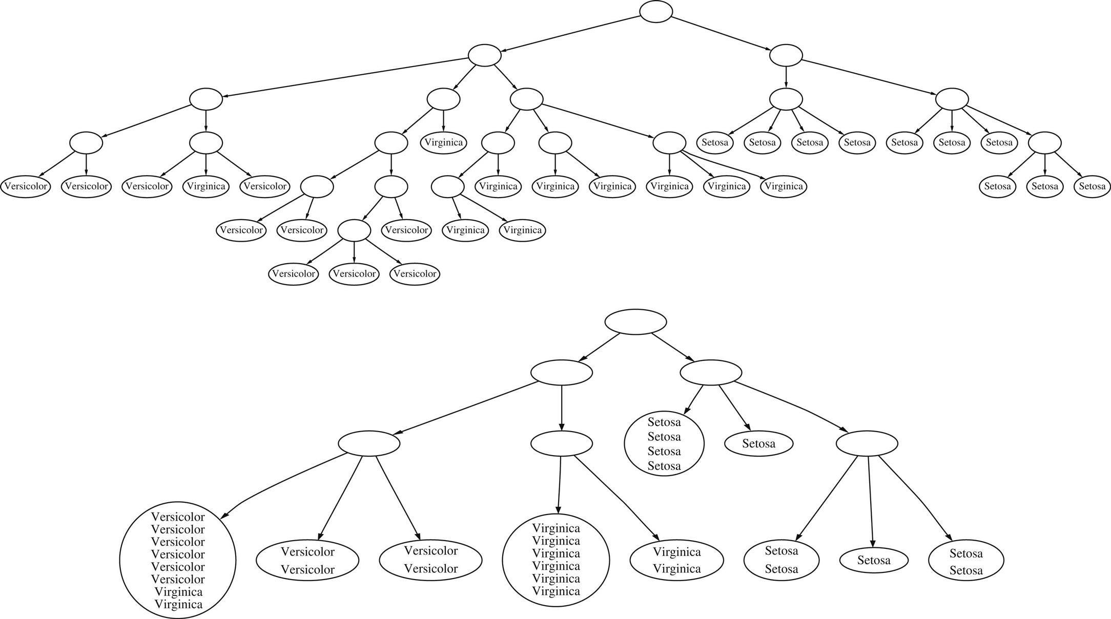
The clusterings produced by this scheme contain one leaf for every instance. This produces an overwhelmingly large hierarchy for datasets of any reasonable size, corresponding, in a sense, to overfitting the particular dataset. Consequently a second numerical parameter called cutoff is used to suppress growth. Some instances are deemed to be sufficiently similar to others to not warrant formation of their own child node, and this parameter governs the similarity threshold. Cutoff is specified in terms of category utility: when the increase in category utility from adding a new node is sufficiently small, that node is cut off.
Fig. 4.21B shows the same iris data, clustered with cutoff in effect. Many leaf nodes contain several instances: these are children of the parent node that have been cut off. The division into the three types of iris is a little easier to see from this hierarchy because some of the detail is suppressed. Again, however, some experimentation with the cutoff parameter was necessary to get this result, and in fact a sharper cutoff leads to much less satisfactory clusters.
Similar clusterings are obtained if the full iris dataset of 150 instances is used. However, the results depend on the ordering of examples: Fig. 4.21 was obtained by alternating the three varieties of iris in the input file. If all I. setosas are presented first, followed by all I. versicolors and then all I. virginicas, the resulting clusters are quite unsatisfactory.
Category Utility
Now we look at how the category utility, which measures the overall quality of a partition of instances into clusters, is calculated. In Section 5.9 we will see how the MDL measure could, in principle, be used to evaluate the quality of clustering. Category utility is not MDL-based but rather resembles a kind of quadratic loss function defined on conditional probabilities.
The definition of category utility is rather formidable:
where C1, C2,…, Ck are the k clusters; the outer summation is over these clusters; the next inner one sums over the attributes; ai is the ith attribute; and it takes on values vi1, vi2,…, which are dealt with by the sum over j. Note that the probabilities themselves are obtained by summing over all instances: thus there is a further implied level of summation.
This expression makes a great deal of sense if you take the time to examine it. The point of having a cluster is that it will give some advantage in predicting the values of attributes of instances in that cluster—i.e., ![]() is a better estimate of the probability that attribute ai has value vij, for an instance in cluster
is a better estimate of the probability that attribute ai has value vij, for an instance in cluster ![]() , than
, than ![]() because it takes account of the cluster the instance is in. If that information doesn’t help, the clusters aren’t doing much good! So what the measure calculates, inside the multiple summation, is the amount by which that information does help in terms of the differences between squares of probabilities. This is not quite the standard squared-difference metric, because that sums the squares of the differences (which produces a symmetric result), and the present measure sums the difference of the squares (which, appropriately, does not produce a symmetric result). The differences between squares of probabilities are summed over all attributes, and all their possible values, in the inner double summation. Then it is summed over all clusters, weighted by their probabilities, in the outer summation.
because it takes account of the cluster the instance is in. If that information doesn’t help, the clusters aren’t doing much good! So what the measure calculates, inside the multiple summation, is the amount by which that information does help in terms of the differences between squares of probabilities. This is not quite the standard squared-difference metric, because that sums the squares of the differences (which produces a symmetric result), and the present measure sums the difference of the squares (which, appropriately, does not produce a symmetric result). The differences between squares of probabilities are summed over all attributes, and all their possible values, in the inner double summation. Then it is summed over all clusters, weighted by their probabilities, in the outer summation.
The overall division by k is a little hard to justify because the squared differences have already been summed over the categories. It essentially provides a “per cluster” figure for the category utility that discourages overfitting. Otherwise, because the probabilities are derived by summing over the appropriate instances, the very best category utility would be obtained by placing each instance in its own cluster. Then, ![]() would be 1 for the value that attribute ai actually has for the single instance in category
would be 1 for the value that attribute ai actually has for the single instance in category ![]() and 0 for all other values; and the numerator of the category utility formula will end up as
and 0 for all other values; and the numerator of the category utility formula will end up as
where n is the total number of attributes. This is the greatest value that the numerator can have; and so if it were not for the additional division by k in the category utility formula, there would never be any incentive to form clusters containing more than one member. This extra factor is best viewed as a rudimentary overfitting-avoidance heuristic.
This category utility formula applies only to nominal attributes. However, it can easily be extended to numeric attributes by assuming that their distribution is normal with a given (observed) mean μ and standard deviation σ. The probability density function for an attribute a is
The analog of summing the squares of attribute–value probabilities is
where σi is the standard deviation of the attribute ai. Thus for a numeric attribute, we estimate the standard deviation from the data, both within the cluster (![]() ) and for the data over all clusters (
) and for the data over all clusters (![]() ), and use these in the category utility formula:
), and use these in the category utility formula:
Now the problem mentioned above that occurs when the standard deviation estimate is zero becomes apparent: a zero standard deviation produces an infinite value of the category utility formula. Imposing a prespecified minimum variance on each attribute, the acuity, is a rough-and-ready solution to the problem.
Remarks
Many of the concepts and techniques presented above are easily adapted to the probabilistic setting, where the task of clustering can be viewed as that of probability density estimation. In Chapter 9, Probabilistic methods, we revisit clustering and examine a statistical clustering based on a mixture model of different probability distributions, one for each cluster. It does not partition instances into disjoint clusters as k-means does, but instead assigns them to classes probabilistically, not deterministically. We explain the basic technique and sketch the working of a comprehensive clustering scheme called AutoClass.
The clustering methods that have been described produce different kinds of output. All are capable of taking new data in the form of a test set and classifying it according to clusters that were discovered by analyzing a training set. However, the hierarchical and incremental clustering methods are the only ones that generate an explicit knowledge structure that describes the clustering in a way that can be visualized and reasoned about. The other algorithms produce clusters that can be visualized in instance space if the dimensionality is not too high.
If a clustering method were used to label the instances of the training set with cluster numbers, that labeled set could then be used to train a rule or decision tree learner. The resulting rules or tree would form an explicit description of the classes. A probabilistic clustering scheme could be used for the same purpose, except that each instance would have multiple weighted labels and the rule or decision tree learner would have to be able to cope with weighted instances—as many can.
Another application of clustering is to fill in any values of the attributes that may be missing. For example, it is possible to make a statistical estimate of the value of unknown attributes of a particular instance, based on the class distribution for the instance itself and the values of the unknown attributes for other examples. We will return to these types of ideas in Chapter 9, Probabilistic methods.
4.9 Multi-instance Learning
In Chapter 2, Input: concepts, instances, attributes, we introduced multi-instance learning, where each example in the data comprises several different instances. We call these examples “bags” (in mathematics, a bag is the same as a set except that particular elements can appear more than once, whereas sets cannot contain duplicates). In supervised multi-instance learning, a class label is associated with each bag, and the goal of learning is to determine how the class can be inferred from the instances that make up the bag. While advanced algorithms have been devised to tackle such problems, it turns out that the “simplicity first” methodology can be applied here with surprisingly good results. A simple but effective approach is to manipulate the input data in such a fashion as to transform it to a single-instance learning problem, and then apply standard learning methods—such as the ones described in this chapter. Two such approaches are described below.
Aggregating the Input
You can convert a multiple-instance problem to a single-instance one by calculating values such as mean, mode, minimum, and maximum that summarize the instances in the bag and adding these as new attributes. Each “summary” instance retains the class label of the bag it was derived from. To classify a new bag the same process is used: a single aggregated instance is created with attributes that summarize the instances in the bag. Surprisingly, for the original drug activity dataset that spurred the development of multi-instance learning, results comparable with special-purpose multi-instance learners can be obtained using just the minimum and maximum values of each attribute for each bag, combined with a support vector machine classifier (see Section 7.2). One potential drawback of this approach is that the best summary statistics to compute depend on the problem at hand. However, the additional computational cost associated with exploring combinations of different summary statistics is offset by the fact that the summarizing process means that fewer instances are processed by the learning algorithm.
Aggregating the Output
Instead of aggregating the instances in each bag, another approach is to learn a classifier directly from the original instances that comprise the bag. To achieve this, the instances in a given bag are all assigned the bag’s class label. At classification time, a prediction is produced for each instance in the bag to be predicted, and the predictions are aggregated in some fashion to form a prediction for the bag as a whole. One approach is to treat the predictions as votes for the various class labels. If the classifier is capable of assigning probabilities to the class labels, these could be averaged to yield an overall probability distribution for the bag’s class label. This method treats the instances independently, and gives them equal influence on the predicted class label.
One problem is that the bags in the training data can contain different numbers of instances. Ideally, each bag should have the same influence on the final model that is learned. If the learning algorithm can accept instance-level weights this can be achieved by assigning each instance in a given bag a weight inversely proportional to the bag’s size. If a bag contains n instances, giving each one a weight of 1/n ensures that the instances contribute equally to the bag’s class label and each bag receives a total weight of 1.
Both these ways of tackling multi-instance problems disregard the original assumption of supervised multi-instance learning that a bag is positive if and only if at least one of its instances is positive. Instead, making each instance in a bag contribute equally to its label is the key element that allows standard learning algorithms to be applied. Otherwise, it is necessary to try to identify the “special” instances that are the key to determining the bag’s label.
4.10 Further Reading and Bibliographic Notes
The 1R scheme was proposed and thoroughly investigated by Holte (1993). It was never really intended as a machine learning “method”: the point was more to demonstrate that very simple structures underlie most of the practical datasets being used to evaluate machine learning schemes at the time and that putting high-powered inductive inference schemes to work on simple datasets was like using a sledgehammer to crack a nut. Why grapple with a complex decision tree when a simple rule will do?
Bayes (1763) was an 18th century English philosopher who set out his theory of probability in an “Essay towards solving a problem in the doctrine of chances,” published in the Philosophical Transactions of the Royal Society of London; the rule that bears his name has been a cornerstone of probability theory ever since. The difficulty with the application of Bayes’ rule in practice is the assignment of prior probabilities. With a particular dataset, prior probabilities for Naïve Bayes are usually reasonably easy to estimate, which encourages a Bayesian approach to learning.
The fact that Naïve Bayes performs well in classification tasks even when the independence assumption that it rests upon is violated was explored by Domingos and Pazzani (1997). Nevertheless, the assumption is a great stumbling block, and there are ways to apply Bayes’ rule without assuming independence. The resulting models are called Bayesian networks (Heckerman, Geiger, & Chickering, 1995), and we describe them in Section 9.2.
Bayesian techniques had been used in the field of pattern recognition (Duda & Hart, 1973) for 20 years before they were adopted by machine learning researchers (e.g., see Langley, Iba, & Thompson, 1992) and made to work on datasets with redundant attributes (Langley & Sage, 1994) and numeric attributes (John & Langley, 1995). The label Naïve Bayes is unfortunate because it is hard to use this method without feeling simpleminded. However, there is nothing naïve about its use in appropriate circumstances. The multinomial Naïve Bayes model, which is particularly useful for text classification, was investigated by McCallum and Nigam (1998).
The classic paper on decision tree induction was written by Quinlan (1986), who described the basic ID3 procedure developed in this chapter. A comprehensive description of the method, including the improvements that are embodied in C4.5, appears in a classic book by Quinlan (1993), which gives a listing of the complete C4.5 system, written in the C programming language. Prism was developed by Cendrowska (1987), who also introduced the contact lens dataset.
Association rules are introduced and described in the database literature rather than in the machine learning literature. Here the emphasis is very much on dealing with huge amounts of data rather than on sensitive ways of testing and evaluating algorithms on limited datasets. The algorithm introduced in this chapter is the Apriori method developed by Agrawal and his associates (Agrawal, Imielinski, & Swami, 1993a, 1993b; Agrawal & Srikant, 1994). A survey of association-rule mining appears in an article by Chen, Jan, and Yu (1996).
Linear regression is described in most standard statistical texts, and a particularly comprehensive treatment can be found in Lawson and Hanson (1995). The use of linear models for classification enjoyed a great deal of popularity in the 1960s; Nilsson (1965) is an excellent reference. He defined a linear threshold unit as a binary test of whether a linear function is greater or less than zero and a linear machine as a set of linear functions, one for each class, whose value for an unknown example was compared and the largest chosen as its predicted class. In the distant past, perceptrons fell out of favor on publication of an influential book that showed that they had fundamental limitations (Minsky & Papert, 1969); however, more complex systems of linear functions have enjoyed a resurgence in recent years in the form of neural networks, described in Section 7.2 and Chapter 10, Deep learning. The Winnow algorithms were introduced by Nick Littlestone in his PhD thesis (Littlestone, 1988, 1989). Multiresponse linear classifiers have found application in an operation called stacking that combines the output of other learning algorithms, described in Chapter 12, Ensemble learning (see Wolpert, 1992).
Fix and Hodges (1951) performed the first analysis of the nearest-neighbor method, and Johns (1961) pioneered its use in classification problems. Cover and Hart (1967) obtained the classic theoretical result that, for large enough datasets, its probability of error never exceeds twice the theoretical minimum; Devroye, Györfi, and Lugosi (1996) showed that k-nearest neighbor is asymptotically optimal for large k and n with k/n→0. Nearest-neighbor methods gained popularity in machine learning through the work of Aha (1992), who showed that instance-based learning can be combined with noisy exemplar pruning and attribute weighting and that the resulting methods perform well in comparison with other learning methods. We take this up again in Chapter 7, Extending instance-based and linear models.
The kD-tree data structure was developed by Friedman, Bentley, and Finkel (1977). Our description closely follows an explanation given by Andrew Moore in his PhD thesis (Moore, 1991), who, along with Omohundro (1987), pioneered its use in machine learning. Moore (2000) described sophisticated ways of constructing ball trees that perform well even with thousands of attributes. We took our ball tree example from lecture notes by Alexander Gray of Carnegie-Mellon University.
The k-means algorithm is a classic technique, and many descriptions and variations are available (e.g., Hartigan, 1975). The k-means++ variant, which yields a significant improvement by choosing the initial seeds more carefully, was introduced as recently as 2007 by Arthur and Vassilvitskii (2007). Our description of how to modify k-means to find a good value of k by repeatedly splitting clusters and seeing whether the split is worthwhile follows the X-means algorithm of Moore and Pelleg (2000). However, instead of the MDL principle they use a probabilistic scheme called the Bayes Information Criterion (Kass & Wasserman, 1995). Efficient agglomerative methods for hierarchical clustering were developed by Day and Edelsbrünner (1984), and the ideas are described in recent books (Duda et al., 2001; Hastie et al., 2009). The incremental clustering procedure, based on the merging and splitting operations, was introduced in systems called Cobweb for nominal attributes (Fisher, 1987) and Classit for numeric attributes (Gennari, Langley, & Fisher, 1990). Both are based on a measure of category utility that had been defined previously (Gluck & Corter, 1985).
A hierarchical clustering method called BIRCH (for “balanced iterative reducing and clustering using hierarchies”) has been developed specifically for large multidimensional datasets, where it is necessary for efficient operation to minimize input–output costs (Zhang, Ramakrishnan, & Livny, 1996). It incrementally and dynamically clusters multidimensional metric data points, seeking the best clustering within given memory and time constraints. It typically finds a good clustering with a single scan of the data, which can then be improved by further scans.
The method of dealing with multi-instance learning problems by applying standard single instance learners to summarize bag-level data was applied in conjunction with support vector machines by Gärtner, Flach, Kowalczyk, and Smola (2002). The alternative approach of aggregating the output was explained by Frank and Xu (2003).
4.11 Weka Implementations
• Inferring rudimentary rules: OneR
NaiveBayes and many variants, including NaiveBayesMultinomial
• Decision trees: Id3 (in the simpleEducationalLearningSchemes package)
• Decision rules: Prism (in the simpleEducationalLearningSchemes package)
SimpleLinearRegression, LinearRegression, Logistic (regression),
Winnow (in the Winnow package)
IB1 (in the simpleEducationalLearningSchemes package)
Cobweb (which includes Classit)
HierarchicalClusterer (hierarchical clustering using various link functions)
SimpleMI, MIWrapper (available in the multi-InstanceLearning package)