
Output
Knowledge representation
Abstract
Having examined the input to machine learning, we move on to review the types of output that can be generated. We first discuss decision tables, which are perhaps the most basic form of knowledge representation, before considering linear models such as those produced by linear regression. Next we explain decision trees, the most widely used kind of knowledge representation in classic machine learning, before looking at rule sets, which are a popular alternative. We consider classification rules, association rules, and rules with exceptions. We briefly venture into the realm of inductive logic programming, which allows for more complex rules than the practical learning techniques covered in this book. Following rules, we discuss instance-based learning and rectangular generalizations. The final section covers the basic types of output generated by clustering techniques: flat clusters and dendrograms.
Keywords
Decision tables; decision trees; classification rules; association rules; inductive logic programming; instance-based learning; rectangular generalizations; clusters; dendrograms
Many of the techniques in this book produce easily comprehensible descriptions of the structural patterns in the data. Before looking at how these techniques work, we have to see how structural patterns can be expressed. There are many different ways for representing the patterns that can be discovered by machine learning, and each one dictates the kind of technique that can be used to infer that output structure from data. Once you understand how the output is represented, you have come a long way toward understanding how it can be generated.
We saw many examples of machine learning in Chapter 1, What’s it all about?. In these cases the output took the form of decision trees and classification rules, which are basic knowledge representation styles that many machine learning methods use. Knowledge is really too imposing a word for a decision tree or a collection of rules, and by using it we don’t really mean to imply that these structures vie with the real kind of knowledge that we carry in our heads: it’s just that we need some word to refer to the structures that learning methods produce. There are more complex varieties of rules that allow exceptions to be specified, and ones that can express relations among the values of the attributes of different instances. Some problems have a numeric class, and—as mentioned in chapter: What’s it all about?—the classic way of dealing with these is to use linear models. Linear models can also be adapted to deal with binary classification. Moreover, special forms of trees can be developed for numeric prediction. Instance-based representations focus on the instances themselves rather than rules that govern their attribute values. Finally, some learning schemes generate clusters of instances. These different knowledge representation methods parallel the different kinds of learning problems introduced in Chapter 2, Input: concepts, instances, attributes.
3.1 Tables
The simplest, most rudimentary way of representing the output from machine learning is to make it just the same as the input—a table. For example, Table 1.2 is a decision table for the weather data: you just look up the appropriate conditions to decide whether or not to play. Exactly the same process can be used for numeric prediction too—in this case, the structure is sometimes referred to as a regression table. Less trivially, creating a decision or regression table might involve selecting some of the attributes. If temperature is irrelevant to the decision, e.g., a smaller, condensed table with that attribute missing would be a better guide. The problem is, of course, to decide which attributes to leave out without affecting the final decision. Attribute selection is discussed in Chapter 8, Data transformations.
3.2 Linear Models
Another simple style of representation is a “linear model,” whose output is just the sum of the attribute values, except that weights are applied to each attribute before adding them together. The trick is to come up with good values for the weights—ones that make the model’s output match the desired output. Here, the output and the inputs—attribute values—are all numeric. Statisticians use the word regression for the process of predicting a numeric quantity, and “linear regression model” is another term for this kind of model. Unfortunately this does not really relate to the ordinary use of the word “regression,” which means to return to a previous state.
Linear models are easiest to visualize in two dimensions, where they are tantamount to drawing a straight line through a set of data points. Fig. 3.1 shows a line fitted to the CPU performance data described in Chapter 1, What’s it all about? (Table 1.5), where only the cache attribute is used as input. The class attribute performance is shown on the vertical axis, with cache on the horizontal axis: both are numeric. The straight line represents the “best fit” prediction equation:

Given a test instance, a prediction can be produced by plugging the observed value of cache into this expression to obtain a value for performance. Here the expression comprises a constant “bias” term (37.06) and a weight for the cache attribute (2.47). Of course, linear models can be extended beyond a single attribute—the trick is to come up with suitable values for each attribute’s weight, and a bias term, that together give a good fit to the training data.
Linear models can also be applied to binary classification problems. In this case, the line produced by the model separates the two classes: it defines where the decision changes from one class value to the other. Such a line is often referred to as the decision boundary. Fig. 3.2 shows a decision boundary for the iris data that separates the Iris setosas from the Iris versicolors. In this case, the data is plotted using two of the input attributes—petal length and petal width—and the straight line defining the decision boundary is a function of these two attributes. Points lying on the line are given by the equation:
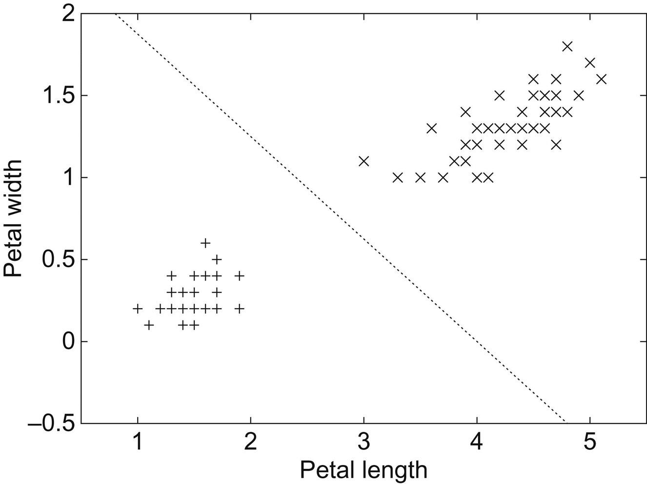
As before, given a test instance, a prediction is produced by plugging the observed values of the attributes in question into the expression. But here we check the result and predict one class if it is greater than or equal to 0 (in this case, Iris setosa) and the other if it is less than 0 (I. versicolor). Again, the model can be extended to multiple attributes, in which case the boundary becomes a high-dimensional plane or “hyperplane” in the instance space. The task is to find values for the weights so that the training data is correctly classified by the hyperplane.
In Figs. 3.1 and 3.2, a different fit to the data could be obtained by changing the position and orientation of the line, i.e., by changing the weights. The weights for Fig. 3.1 were found by a method called least squares linear regression; those for Fig. 3.2 were found by the perceptron training rule. Both methods are described in Chapter 4, Algorithms: the basic methods.
3.3 Trees
A “divide-and-conquer” approach to the problem of learning from a set of independent instances leads naturally to a style of representation called a decision tree. We have seen some examples of decision trees, for the contact lens (Fig. 1.2) and labor negotiations (Fig. 1.3) datasets. Nodes in a decision tree involve testing a particular attribute. Usually, the test compares an attribute value with a constant. Leaf nodes give a classification that applies to all instances that reach the leaf, or a set of classifications, or a probability distribution over all possible classifications. To classify an unknown instance, it is routed down the tree according to the values of the attributes tested in successive nodes, and when a leaf is reached the instance is classified according to the class assigned to the leaf.
If the attribute that is tested at a node is a nominal one, the number of children is usually the number of possible values of the attribute. In this case, because there is one branch for each possible value, the same attribute will not be retested further down the tree. Sometimes the attribute values are divided into two subsets, and the tree branches just two ways depending on which subset the value lies in the tree; in that case, the attribute might be tested more than once in a path.
If the attribute is numeric, the test at a node usually determines whether its value is greater or less than a predetermined constant, giving a two-way split. Alternatively, a three-way split may be used, in which case there are several different possibilities. If missing value is treated as an attribute value in its own right, that will create a third branch. An alternative for an integer-valued attribute would be a three-way split into less than, equal to, and greater than. An alternative for a real-valued attribute, for which equal to is not such a meaningful option, would be to test against an interval rather than a single constant, again giving a three-way split: below, within, and above. A numeric attribute is often tested several times in any given path down the tree from root to leaf, each test involving a different constant. We return to this when describing the handling of numeric attributes in Section 6.1.
Missing values pose an obvious problem. It is not clear which branch should be taken when a node tests an attribute whose value is missing. Sometimes, as described in Section 2.4, missing value is treated as an attribute value in its own right. If this is not the case, missing values should be treated in a special way rather than being considered just another possible value that the attribute might take. A simple solution is to record the number of elements in the training set that go down each branch and to use the most popular branch if the value for a test instance is missing.
A more sophisticated solution is to notionally split the instance into pieces and send part of it down each branch and from there right on down to the leaves of the subtrees involved. The split is accomplished using a numeric weight between 0 and 1, and the weight for a branch is chosen to be proportional to the number of training instances going down that branch, all weights summing to 1. A weighted instance may be further split at a lower node. Eventually, the various parts of the instance will each reach a leaf node, and the decisions at these leaf nodes must be recombined using the weights that have percolated down to the leaves. We return to this in Section 6.1.
So far we’ve described decision trees that divide the data at a node by comparing the value of some attribute with a constant. This is the most common approach. If you visualize this with two input attributes in two dimensions, comparing the value of one attribute with a constant splits the data parallel to that axis. However, there are other possibilities. Some trees compare two attributes with one another, while others compute some function of several attributes. For example, using a hyperplane as described in Section 3.2 results in an oblique split that is not parallel to an axis. A functional tree can have oblique splits as well as linear models at the leaf nodes, which are used for prediction. It is also possible for some nodes in the tree to specify alternative splits on different attributes, as though the tree designer couldn’t make up their mind which one to choose. This might be useful if the attributes seem to be equally useful for classifying the data. Such nodes are called option nodes, and when classifying an unknown instance all branches leading from an option node are followed. This means that the instance will end up in more than one leaf, giving various alternative predictions, which are then combined in some fashion—e.g., using majority voting.
It is instructive and can even be entertaining to build a decision tree for a dataset manually. To do so effectively, you need a good way of visualizing the data so that you can decide which are likely to be the best attributes to test and what an appropriate test might be. The Weka Explorer, described in Appendix B, has a User Classifier facility that allows users to construct a decision tree interactively. It presents you with a scatter plot of the data against two selected attributes, which you choose. When you find a pair of attributes that discriminates the classes well, you can create a two-way split by drawing a polygon around the appropriate data points on the scatter plot.
For example, in Fig. 3.3A the user is operating on a dataset with three classes, the iris dataset, and has found two attributes, petallength and petalwidth, that do a good job of splitting up the classes. A rectangle has been drawn, manually, to separate out one of the classes (I. versicolor). Then the user switches to the decision tree view in Fig. 3.3B to see the tree so far. The left-hand leaf node contains predominantly irises of one type (I. versicolor, contaminated by only one virginica); the right-hand one contains predominantly two types (I. setosa and virginica, contaminated by only three versicolors). The user will probably select the right-hand leaf and work on it next, splitting it further with another rectangle—perhaps based on a different pair of attributes (although, from Fig. 3.3A, these two look pretty good).

The kinds of decision trees we’ve been looking at are designed for predicting categories rather than numeric quantities. When it comes to predicting numeric quantities, as with the CPU performance data in Table 1.5, the same kind of tree can be used, but each leaf would contain a numeric value that is the average of all the training set values to which the leaf applies. Because a numeric quantity is what is predicted, decision trees with averaged numeric values at the leaves are called regression trees.
Fig. 3.4A shows a regression equation for the CPU performance data, and Fig. 3.4B shows a regression tree. The leaves of the tree are numbers that represent the average outcome for instances that reach the leaf. The tree is much larger and more complex than the regression equation, and if we calculate the average of the absolute values of the errors between the predicted and actual CPU performance measures, it turns out to be significantly less for the tree than for the regression equation. The regression tree is more accurate because a simple linear model poorly represents the data in this problem. However, the tree is cumbersome and difficult to interpret because of its large size.
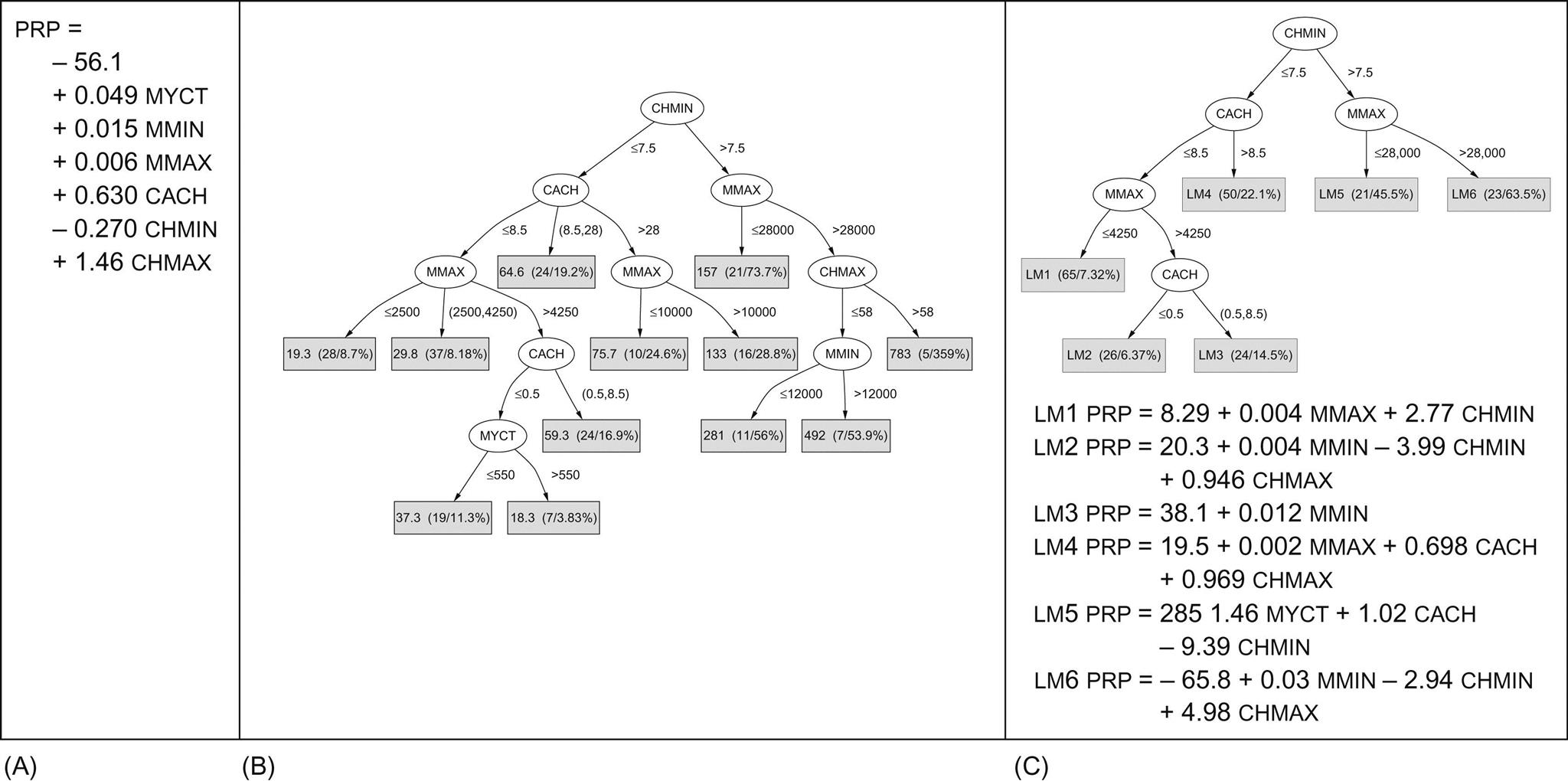
It is possible to combine regression equations with regression trees. Fig. 3.4C is a tree whose leaves contain linear expressions—i.e., regression equations—rather than single predicted values. This is called a model tree. Fig. 3.4C contains the six linear models that belong at the six leaves, labeled LM1 through LM6. The model tree approximates continuous functions by linear “patches,” a more sophisticated representation than either linear regression or regression trees. Although the model tree is smaller and more comprehensible than the regression tree, the average error values on the training data are lower. (However, we will see in Chapter 5, Credibility: evaluating what’s been learned, that calculating the average error on the training set is not in general a good way of assessing the performance of models.)
3.4 Rules
Rules are a popular alternative to decision trees, and we have already seen examples for the weather, contact lens, iris, and soybean datasets. The antecedent, or precondition, of a rule is a series of tests just like the tests at nodes in decision trees, while the consequent, or conclusion, gives the class or classes that apply to instances covered by that rule, or perhaps gives a probability distribution over the classes. Generally, the preconditions are logically ANDed together, and all the tests must succeed if the rule is to fire. However, in some rule formulations the preconditions are general logical expressions rather than simple conjunctions. We often think of the individual rules as being effectively logically ORed together: if any one applies, the class (or probability distribution) given in its conclusion is applied to the instance. However, conflicts arise when several rules with different conclusions apply; we will return to this shortly.
Classification Rules
It is easy to read a set of classification rules directly off a decision tree. One rule is generated for each leaf. The antecedent of the rule includes a condition for every node on the path from the root to that leaf, and the consequent of the rule is the class assigned by the leaf. This procedure produces rules that are unambiguous in that the order in which they are executed is irrelevant. However, in general, rules that are read directly off a decision tree are far more complex than necessary, and rules derived from trees are usually pruned to remove redundant tests.
Because decision trees cannot easily express the disjunction implied among the different rules in a set, transforming a general set of rules into a tree is not quite so straightforward. A good illustration of this occurs when the rules have the same structure but different attributes, like:
If a and b then x
If c and d then x
Then it is necessary to break the symmetry and choose a single test for the root node. If, e.g., a is chosen, the second rule must, in effect, be repeated twice in the tree, as shown in Fig. 3.5. This is known as the replicated subtree problem.

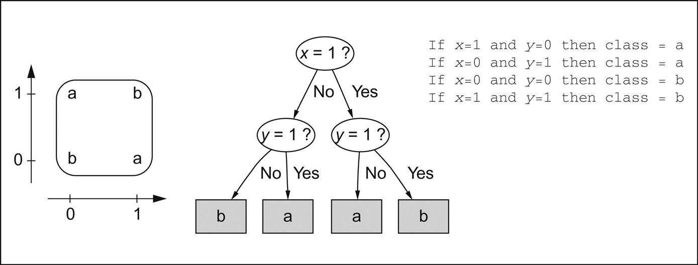
The replicated subtree problem is sufficiently important that it is worth looking at a couple more examples. The diagram on the left of Fig. 3.6 shows an exclusive-or function for which the output is a if x=1 or y=1 but not both. To make this into a tree, you have to split on one attribute first, leading to a structure like the one shown in the center. In contrast, rules can faithfully reflect the true symmetry of the problem with respect to the attributes, as shown on the right.
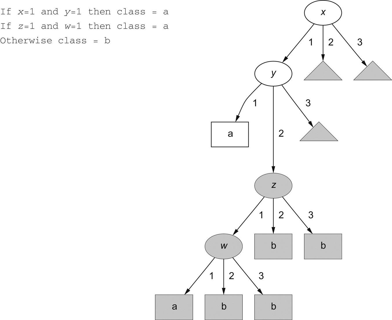
In this example the rules are not notably more compact than the tree. In fact, they are just what you would get by reading rules off the tree in the obvious way. But in other situations, rules are much more compact than trees, particularly if it is possible to have a “default” rule that covers cases not specified by the other rules. For example, to capture the effect of the rules in Fig. 3.7, in which there are four attributes—x, y, z, and w, which can each be 1, 2, or 3—requires the tree shown on the right. Each of the three small gray triangles to the upper right should actually contain the whole three-level subtree that is displayed in gray, a rather extreme example of the replicated subtree problem. This is a distressingly complex description of a rather simple concept.
One reason why rules are popular is that each rule seems to represent an independent “nugget” of knowledge. New rules can be added to an existing rule set without disturbing ones already there, whereas to add to a tree structure may require reshaping the whole tree. However, this independence is something of an illusion, because it ignores the question of how the rule set is executed. We explained earlier the fact that if rules are meant to be interpreted in order as a “decision list,” some of them, taken individually and out of context, may be incorrect. On the other hand, if the order of interpretation is supposed to be immaterial, then it is not clear what to do when different rules lead to different conclusions for the same instance. This situation cannot arise for rules that are read directly off a decision tree because the redundancy included in the structure of the rules prevents any ambiguity in interpretation. But it does arise when rules are generated in other ways.
If a rule set gives multiple classifications for a particular example, one solution is to give no conclusion at all. Another is to count how often each rule fires on the training data and go with the most popular one. These strategies can lead to radically different results. A different problem occurs when an instance is encountered that the rules fail to classify at all. Again, this cannot occur with decision trees, or with rules read directly off them, but it can easily happen with general rule sets. One way of dealing with this situation is to fail to classify such an example; another is to choose the most frequently occurring class as a default. Again, radically different results may be obtained for these strategies. Individual rules are simple, and sets of rules seem deceptively simple—but given just a set of rules with no additional information, it is not clear how it should be interpreted.
A particularly straightforward situation occurs when rules lead to a class that is Boolean (say, yes and no), and when only rules leading to one outcome (say, yes) are expressed. The assumption is that if a particular instance is not in class yes, then it must be in class no—a form of closed world assumption. If this is the case, rules cannot conflict and there is no ambiguity in rule interpretation: any interpretation strategy will give the same result. Such a set of rules can be written as a logic expression in what is called disjunctive normal form: i.e., as a disjunction (OR) of conjunctive (ANDed) conditions.
It is this simple special case that seduces people into assuming that rules are very easy to deal with, for here each rule really does operate as a new, independent piece of information that contributes in a straightforward way to the disjunction. Unfortunately, it only applies to Boolean outcomes and requires the closed world assumption, and these constraints are unrealistic in many practical situations. Machine learning algorithms that generate rules invariably produce ordered rule sets in multiclass situations, and this sacrifices any possibility of modularity because the order of execution is critical.
Association Rules
Association rules are no different from classification rules except that they can predict any attribute, not just the class, and this gives them the freedom to predict combinations of attributes too. Also, association rules are not intended to be used together as a set, as classification rules are. Different association rules express different regularities that underlie the dataset, and they generally predict different things.
Because so many different association rules can be derived from even a tiny dataset, interest is restricted to those that apply to a reasonably large number of instances and have a reasonably high accuracy on the instances to which they apply. The coverage of an association rule is the number of instances for which it predicts correctly—this is often called its support. Its accuracy—often called confidence—is the number of instances that it predicts correctly, expressed as a proportion of all instances to which it applies. For example, with the rule:
If temperature = cool then humidity = normal
the coverage is the number of days that are both cool and have normal humidity (4 in the data of Table 1.2), and the accuracy is the proportion of cool days that have normal humidity (100% in this case). It is usual to specify minimum coverage and accuracy values, and to seek only those rules whose coverage and accuracy are both at least these specified minima. In the weather data, e.g., there are 58 rules whose coverage and accuracy are at least 2 and 95%, respectively. (It may also be convenient to specify coverage as a percentage of the total number of instances instead.)
Association rules that predict multiple consequences must be interpreted rather carefully. For example, with the weather data in Table 1.2 we saw this rule:
If windy = false and play = no then outlook = sunny
and humidity = high.
This is not just a shorthand expression for the two separate rules:
If windy = false and play = no then outlook = sunny
If windy = false and play = no then humidity = high
It does indeed imply that these exceed the minimum coverage and accuracy figures—but it also implies more. The original rule means that the number of examples that are nonwindy, nonplaying, with sunny outlook and high humidity, is at least as great as the specified minimum coverage figure. It also means that the number of such days, expressed as a proportion of nonwindy, nonplaying days, is at least the specified minimum accuracy figure. This implies that the rule
If humidity = high and windy = false and play = no then outlook = sunny
also holds, because it has the same coverage as the original rule, and its accuracy must be at least as high as the original rule’s because the number of high-humidity, nonwindy, nonplaying days is necessarily less than that of nonwindy, nonplaying days—which makes the accuracy greater.
As we have seen, there are relationships between particular association rules: some rules imply others. To reduce the number of rules that are produced, in cases where several rules are related it makes sense to present only the strongest one to the user. In the above example, only the first rule should be printed.
Rules With Exceptions
Returning to classification rules, a natural extension is to allow them to have exceptions. Then incremental modifications can be made to a rule set by expressing exceptions to existing rules rather than reengineering the entire set. For example, consider the iris problem described earlier. Suppose a new flower was found with the dimensions given in Table 3.1, and an expert declared it to be an instance of I. setosa. If this flower was classified by the rules given in Chapter 1, What’s it all about?, for this problem, it would be misclassified by two of them:
Table 3.1
| Sepal Length | Sepal Width | Petal Length | Petal Width | Type |
| 5.1 | 3.5 | 2.6 | 0.2 | ? |

If petal-length ≥ 2.45 and petal-length < 4.45 then Iris-versicolor
If petal-length ≥ 2.45 and petal-length < 4.95 and petal-width < 1.55 then Iris-versicolor
These rules require modification so that the new instance can be treated correctly. However, simply changing the bounds for the attribute–value tests in these rules may not suffice because the instances used to create the rule set may then be misclassified. Fixing up a rule set is not as simple as it sounds.
Instead of changing the tests in the existing rules, an expert might be consulted to explain why the new flower violates them, giving explanations that could be used to extend the relevant rules only. For example, the first of these two rules misclassifies the new I. setosa as an instance of the genus I. versicolor. Instead of altering the bounds on any of the inequalities in the rule, an exception can be made based on some other attribute:
If petal-length ≥ 2.45 and petal-length < 4.45 then Iris-versicolor EXCEPT if petal-width < 1.0 then Iris-setosa
This rule says that a flower is I. versicolor if its petal length is between 2.45 and 4.45 cm except when its petal width is less than 1.0 cm, in which case it is I. setosa.
Of course, we might have exceptions to the exceptions, exceptions to these, and so on, giving the rule set something of the character of a tree. As well as being used to make incremental changes to existing rule sets, rules with exceptions can be used to represent the entire concept description in the first place.
Fig. 3.8 shows a set of rules that correctly classify all examples in the iris dataset given earlier. These rules are quite difficult to comprehend at first. Let’s follow them through. A default outcome has been chosen, I. setosa, and is shown in the first line. For this dataset, the choice of default is rather arbitrary because there are 50 examples of each type. Normally, the most frequent outcome is chosen as the default.

Subsequent rules give exceptions to this default. The first if … then, on lines 2 through 4, gives a condition that leads to the classification I. versicolor. However, there are two exceptions to this rule (lines 5 through 8), which we will deal with in a moment. If the conditions on lines 2 and 3 fail, the else clause on line 9 is reached, which essentially specifies a second exception to the original default. If the condition on line 9 holds, the classification is Iris virginica (line 10). Again, there is an exception to this rule (on lines 11 and 12).
Now return to the exception on lines 5 through 8. This overrides the I. versicolor conclusion on line 4 if either of the tests on lines 5 and 7 holds. As it happens, these two exceptions both lead to the same conclusion, I. virginica (lines 6 and 8). The final exception is the one on lines 11 and 12, which overrides the I. virginica conclusion on line 10 when the condition on line 11 is met, and leads to the classification I. versicolor.
You will probably need to ponder these rules for some minutes before it becomes clear how they are intended to be read. Although it takes some time to get used to reading them, sorting out the excepts and if … then … elses becomes easier with familiarity. People often think of real problems in terms of rules, exceptions, and exceptions to the exceptions, so it is often a good way to express a complex rule set. But the main point in favor of this way of representing rules is that it scales up well. Although the whole rule set is a little hard to comprehend, each individual conclusion, each individual then statement, can be considered just in the context of the rules and exceptions that lead to it; whereas with decision lists, all prior rules need to be reviewed to determine the precise effect of an individual rule. This locality property is crucial when trying to understand large rule sets. Psychologically, people familiar with the data think of a particular set of cases, or kind of case, when looking at any one conclusion in the exception structure, and when one of these cases turns out to be an exception to the conclusion, it is easy to add an except clause to cater for it.
It is worth pointing out that the default … except if … then … structure is logically equivalent to an if … then … else …, where the else is unconditional and specifies exactly what the default did. An unconditional else is, of course, a default. (Note that there are no unconditional elses in the preceding rules.) Logically, the exception-based rules can very simply be rewritten in terms of regular if … then … else clauses. What is gained by the formulation in terms of exceptions is not logical but psychological. We assume that the defaults and the tests that occur early on apply more widely than the exceptions further down. If this is indeed true for the domain, and the user can see that it is plausible, the expression in terms of (common) rules and (rare) exceptions will be easier to grasp than a different, but logically equivalent, structure.
More Expressive Rules
We have assumed implicitly that the conditions in rules involve testing an attribute value against a constant. But this may not be ideal. Suppose, to take a concrete example, we have the set of eight building blocks of the various shapes and sizes illustrated in Fig. 3.9, and we wish to learn the concept of standing up. This is a classic two-class problem with classes standing and lying. The four shaded blocks are positive (standing) examples of the concept, and the unshaded blocks are negative (lying) examples. The only information the learning algorithm will be given is the width, height, and number of sides of each block. The training data is shown in Table 3.2.
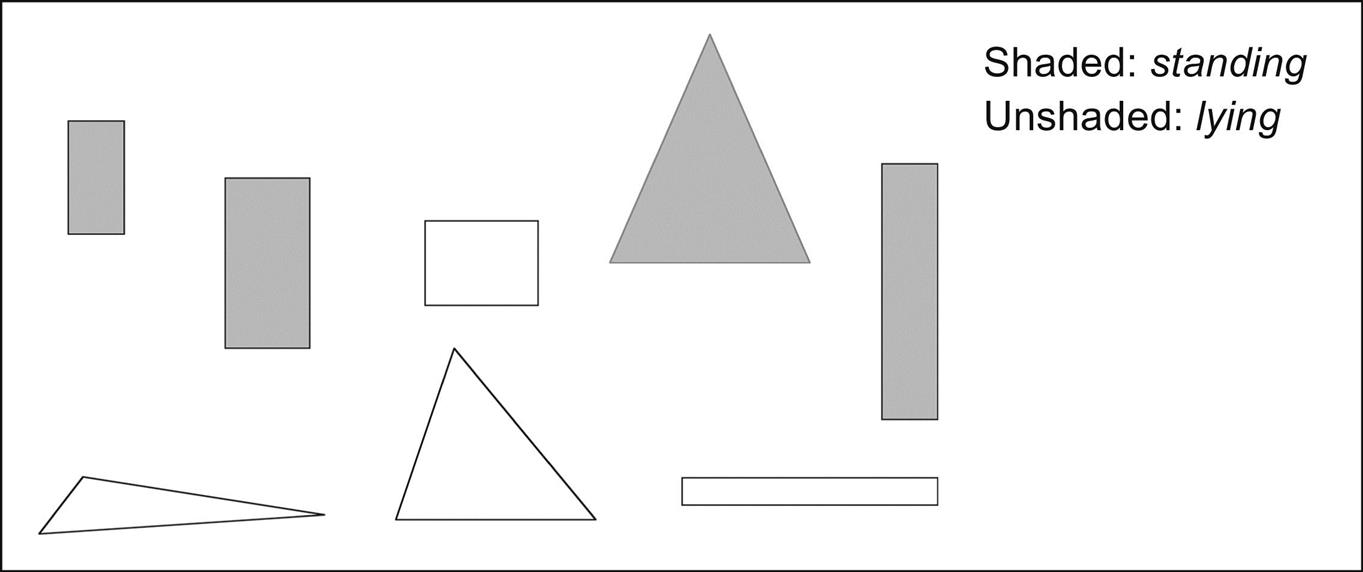
Table 3.2
Training Data for the Shapes Problem
| Width | Height | Sides | Class |
| 2 | 4 | 4 | Standing |
| 3 | 6 | 4 | Standing |
| 4 | 3 | 4 | Lying |
| 7 | 8 | 3 | Standing |
| 7 | 6 | 3 | Lying |
| 2 | 9 | 4 | Standing |
| 9 | 1 | 4 | Lying |
| 10 | 2 | 3 | Lying |

A conventional rule set that might be produced for this data is:
if width ≥ 3.5 and height < 7.0 then lying
if height ≥ 3.5 then standing
In case you’re wondering, 3.5 is chosen as the breakpoint for width because it is halfway between the width of the thinnest lying block, namely 4, and the width of the fattest standing block whose height is less than 7, namely 3. Also, 7.0 is chosen as the breakpoint for height because it is halfway between the height of the tallest lying block, namely 6, and the shortest standing block whose width is greater than 3.5, namely 8. It is common to place numeric thresholds halfway between the values that delimit the boundaries of a concept.
Although these two rules work well on the examples given, they are not very good. Many new blocks would not be classified by either rule (e.g., one with width 1 and height 2), and it is easy to devise many legitimate blocks that the rules would not fit.
A person classifying the eight blocks would probably notice that “standing blocks are those that are taller than they are wide.” This rule does not compare attribute values with constants, it compares attributes with one another:
if width > height then lying
if height > width then standing
The actual values of the height and width attributes are not important: just the result of comparing the two.
Many machine learning schemes do not consider relations between attributes because there is a considerable cost in doing so. One way of rectifying this is to add extra, secondary attributes that say whether two primary attributes are equal or not, or give the difference between them if they are numeric. For example, we might add a binary attribute is width < height? to Table 3.2. Such attributes are often added as part of the data engineering process.
With a seemingly rather small further enhancement, the expressive power of the knowledge representation can be extended very greatly. The trick is to express rules in a way that makes the role of the instance explicit:
if width(block) > height(block) then lying(block)
if height(block) > width(block) then standing(block)
Although this may not seem like much of an extension, it is if instances can be decomposed into parts. For example, if a tower is a pile of blocks, one on top of the other, the fact that the topmost block of the tower is standing can be expressed by:
if height(tower.top) > width(tower.top) then standing(tower.top)
Here, tower.top is used to refer to the topmost block. So far, nothing has been gained. But if tower.rest refers to the rest of the tower, then the fact that the tower is composed entirely of standing blocks can be expressed by the rules:
if height(tower.top) > width(tower.top) and standing(tower.rest) then standing(tower)
The apparently minor addition of the condition standing(tower.rest) is a recursive expression that will turn out to be true only if the rest of the tower is composed of standing blocks. That will be tested by a recursive application of the same rule. Of course, it is necessary to ensure that the recursion “bottoms out” properly by adding a further rule, such as:
if tower = empty then standing(tower.top)
Sets of rules like this are called logic programs, and this area of machine learning is called inductive logic programming. We will not be treating it further in this book.
3.5 Instance-Based Representation
The simplest form of learning is plain memorization, or rote learning. Once a set of training instances has been memorized, on encountering a new instance the memory is searched for the training instance that most strongly resembles the new one. The only problem is how to interpret “resembles”: we will explain that shortly. First, however, note that this is a completely different way of representing the “knowledge” extracted from a set of instances: just store the instances themselves and operate by relating new instances whose class is unknown to existing ones whose class is known. Instead of trying to create rules, work directly from the examples themselves. This is known as instance-based learning. In a sense all the other learning methods are “instance-based” too, because we always start with a set of instances as the initial training information. But the instance-based knowledge representation uses the instances themselves to represent what is learned, rather than inferring a rule set or decision tree and storing it instead.
In instance-based learning, all the real work is done when the time comes to classify a new instance rather than when the training set is processed. In a sense, then, the difference between this method and the others that we have seen is the time at which the “learning” takes place. Instance-based learning is lazy, deferring the real work as long as possible, whereas other methods are eager, producing a generalization as soon as the data has been seen. In instance-based classification, each new instance is compared with existing ones using a distance metric, and the closest existing instance is used to assign the class to the new one. This is called the nearest-neighbor classification method. Sometimes more than one nearest neighbor is used, and the majority class of the closest k neighbors (or the distance-weighted average, if the class is numeric) is assigned to the new instance. This is termed the k-nearest-neighbor method.
Computing the distance between two examples is trivial when examples have just one numeric attribute: it is just the difference between the two attribute values. It is almost as straightforward when there are several numeric attributes: generally, the standard Euclidean distance is used. However, this assumes that the attributes are normalized and are of equal importance, and one of the main problems in learning is to determine which are the important features.
When nominal attributes are present, it is necessary to come up with a “distance” between different values of that attribute. What are the distances between, say, the values red, green, and blue? Usually a distance of zero is assigned if the values are identical; otherwise, the distance is one. Thus the distance between red and red is zero but that between red and green is one. However, it may be desirable to use a more sophisticated representation of the attributes. For example, with more colors one could use a numeric measure of hue in color space, making yellow closer to orange than it is to green and ocher closer still.
Some attributes will be more important than others, and this is usually reflected in the distance metric by some kind of attribute weighting. Deriving suitable attribute weights from the training set is a key problem in instance-based learning.
It may not be necessary, or desirable, to store all the training instances. For one thing, this may make the nearest-neighbor calculation unbearably slow. For another, it may consume unrealistic amounts of storage. Generally some regions of attribute space are more stable than others with regard to class, and just a few exemplars are needed inside stable regions. For example, you might expect the required density of exemplars that lie well inside class boundaries to be much less than the density that is needed near class boundaries. Deciding which instances to save and which to discard is another key problem in instance-based learning.
An apparent drawback to instance-based representations is that they do not make explicit the structures that are learned. In a sense this violates the notion of “learning” that we presented at the beginning of this book; instances do not really “describe” the patterns in data. However, the instances combine with the distance metric to carve out boundaries in instance space that distinguish one class from another, and this is a kind of explicit representation of knowledge. For example, given a single instance of each of two classes, the nearest-neighbor rule effectively splits the instance space along the perpendicular bisector of the line joining the instances. Given several instances of each class, the space is divided by a set of lines that represent the perpendicular bisectors of selected lines joining an instance of one class to one of another class. Fig. 3.10A illustrates a nine-sided polygon that separates the filled-circle class from the open-circle class. This polygon is implicit in the operation of the nearest-neighbor rule.

When training instances are discarded, the result is to save just a few critical examples of each class. Fig. 3.10B shows only the examples that actually get used in nearest-neighbor decisions: the others (the light gray ones) can be discarded without affecting the result. These examples serve as a kind of explicit knowledge representation.
Some instance-based representations go further and explicitly generalize the instances. Typically this is accomplished by creating rectangular regions that enclose examples of the same class. Fig. 3.10C shows the rectangular regions that might be produced. Unknown examples that fall within one of the rectangles will be assigned the corresponding class: ones that fall outside all rectangles will be subject to the usual nearest-neighbor rule. Of course this produces different decision boundaries from the straightforward nearest-neighbor rule, as can be seen by superimposing the polygon in Fig. 3.10A onto the rectangles. Any part of the polygon that lies within a rectangle will be chopped off and replaced by the rectangle’s boundary.
Rectangular generalizations in instance space are just like rules with a special form of condition, one that tests a numeric variable against an upper and lower bound and selects the region in between. Different dimensions of the rectangle correspond to tests on different attributes being ANDed together. Choosing snugly fitting rectangular regions as tests leads to much more conservative rules than those generally produced by rule-based machine learning schemes, because for each boundary of the region, there is an actual instance that lies on (or just inside) that boundary. Tests such as x < a (where x is an attribute value and a is a constant) encompass an entire half-space—they apply no matter how small x is as long as it is less than a. When doing rectangular generalization in instance space you can afford to be conservative because if a new example is encountered that lies outside all regions, you can fall back on the nearest-neighbor metric. With rule-based methods the example cannot be classified, or receives just a default classification, if no rules apply to it. The advantage of more conservative rules is that, although incomplete, they may be more perspicuous than a complete set of rules that covers all cases. Finally, ensuring that the regions do not overlap is tantamount to ensuring that at most one rule can apply to an example, eliminating another of the difficulties of rule-based systems—what to do when several rules apply.
A more complex kind of generalization is to permit rectangular regions to nest one within another. Then a region that is basically all one class can contain an inner region with a different class, as illustrated in Fig. 3.10D. It is possible to allow nesting within nesting so that the inner region can itself contain its own inner region of a different class—perhaps the original class of the outer region. This is analogous to allowing rules to have exceptions and exceptions to the exceptions, as in Section 3.5.
It is worth pointing out a slight danger to the technique of visualizing instance-based learning in terms of boundaries in example space: it makes the implicit assumption that attributes are numeric rather than nominal. If the various values that a nominal attribute can take on were laid out along a line, generalizations involving a segment of that line would make no sense: each test involves either one value for the attribute or all values for it (or perhaps an arbitrary subset of values). Although you can more or less easily imagine extending the examples in Fig. 3.10 to several dimensions, it is much harder to imagine how rules involving nominal attributes will look in multidimensional instance space. Many machine learning situations involve numerous attributes, and our intuitions tend to lead us astray when extended to high-dimensional spaces.
3.6 Clusters
When clusters rather than a classifier is learned, the output takes the form of a diagram that shows how the instances fall into clusters. In the simplest case this involves associating a cluster number with each instance, which might be depicted by laying the instances out in two dimensions and partitioning the space to show each cluster, as illustrated in Fig. 3.11A.
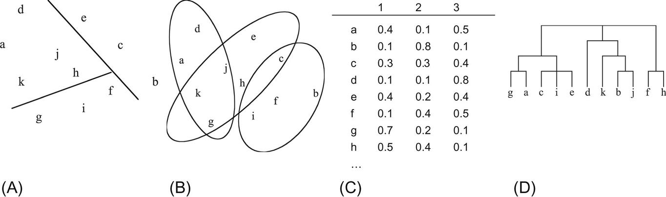
Some clustering algorithms allow one instance to belong to more than one cluster, so the diagram might lay the instances out in two dimensions and draw overlapping subsets representing each cluster—a Venn diagram, as in Fig. 3.11B. Some algorithms associate instances with clusters probabilistically rather than categorically. In this case, for every instance there is a probability or degree of membership with which it belongs to each of the clusters. This is shown in Fig. 3.11C. This particular association is meant to be a probabilistic one, so the numbers for each example sum to one—although that is not always the case. Other algorithms produce a hierarchical structure of clusters so that at the top level the instance space divides into just a few clusters, each of which divides into its own subclusters at the next level down, and so on. In this case a diagram such as the one in Fig. 3.11D is used, in which elements joined together at lower levels are more tightly clustered than ones joined together at higher levels. Such diagrams are called dendrograms. This term means just the same thing as tree diagrams (the Greek word dendron means a “tree”), but in clustering the more exotic version seems to be preferred—perhaps because biological species are a prime application area for clustering techniques, and ancient languages are often used for naming in biology.
Clustering is often followed by a stage in which a decision tree or rule set is inferred that allocates each instance to the cluster in which it belongs. Then, the clustering operation is just one step on the way to a structural description.
3.7 Further Reading and Bibliographic Notes
Knowledge representation is a key topic in classical artificial intelligence and early work is well represented by a comprehensive series of papers edited by Brachman and Levesque (1985). The area of inductive logic programming and associated topics are well covered by de Raedt’s (2008) book Logical and relational learning.
We mentioned the problem of dealing with conflict among different rules. Various ways of doing this, called conflict resolution strategies, have been developed for use with rule-based programming systems. These are described in books on rule-based programming, such as Brownstown, Farrell, Kant, and Martin (1985). Again, however, they are designed for use with handcrafted rule sets rather than ones that have been learned. The use of handcrafted rules with exceptions for a large dataset has been studied by Gaines and Compton (1995), and Richards and Compton (1998) describe their role as an alternative to classic knowledge engineering.
Further information on the various styles of concept representation can be found in the papers that describe machine learning methods for inferring concepts from examples, and these are covered in the Further reading section of Chapter 4, Algorithms: the basic methods, and the Discussion sections of Chapter 6, Trees and rules, and Chapter 7, Extending instance-based and linear models. Finally, graphical models for representing concepts in the form of probability distributions are discussed in Chapter 9, Probabilistic methods.