
What’s it all about?
Abstract
This book is about machine learning techniques for data mining. We start by explaining what people mean by data mining and machine learning, and give some simple example machine learning problems, including both classification and numeric prediction tasks, to illustrate the kinds of input and output involved. To demonstrate the wide applicability of machine learning in practical applications, we continue with brief reviews of several fielded applications from a diverse set of areas. Machine learning is closely linked to the study of statistics, and we discuss the connections between these two fields next. It is also strongly related to the field of artificial intelligence, particularly search techniques, and we devote a section to investigating this relationship. We conclude the chapter by discussing the ethical issues involved when applying data mining in practice.
Keywords
Machine learning; data mining; classification; numeric prediction; data mining applications; machine learning and statistics; generalization as search; data mining and ethics
Human in vitro fertilization involves collecting several eggs from a woman’s ovaries, which, after fertilization with partner or donor sperm, produce several embryos. Some of these are selected and transferred to the woman’s uterus. The problem is to select the “best” embryos to use—the ones that are most likely to survive. Selection is based on around 60 recorded features of the embryos—characterizing their morphology, oocyte, follicle, and sperm sample. The number of features is sufficiently large that it is difficult for an embryologist to assess them all simultaneously and correlate historical data with the crucial outcome of whether that embryo did or did not result in a live child. In a research project in England, machine learning has been investigated as a technique for making the selection, using historical records of embryos and their outcome as training data.
Every year, dairy farmers in New Zealand have to make a tough business decision: which cows to retain in their herd and which to sell off to an abattoir. Typically, one-fifth of the cows in a dairy herd are culled each year near the end of the milking season as feed reserves dwindle. Each cow’s breeding and milk production history influences this decision. Other factors include age (a cow is nearing the end of its productive life at 8 years), health problems, history of difficult calving, undesirable temperament traits (kicking or jumping fences), and not being in calf for the following season. About 700 attributes for each of several million cows have been recorded over the years. Machine learning has been investigated as a way of ascertaining what factors are taken into account by successful farmers—not to automate the decision but to propagate their skills and experience to others.
Life and death. From Europe to the antipodes. Family and business. Machine learning is a burgeoning new technology for mining knowledge from data, a technology that a lot of people are starting to take seriously.
1.1 Data Mining and Machine Learning
We are overwhelmed with data. The amount of data in the world, in our lives, seems ever-increasing—and there’s no end in sight. Omnipresent computers make it too easy to save things that previously we would have trashed. Inexpensive disks and online storage make it too easy to postpone decisions about what to do with all this stuff—we simply get more memory and keep it all. Ubiquitous electronics record our decisions, our choices in the supermarket, our financial habits, our comings and goings. We swipe our way through the world, every swipe a record in a database. The World Wide Web overwhelms us with information; meanwhile, every choice we make is recorded. And all these are just personal choices: they have countless counterparts in the world of commerce and industry. We would all testify to the growing gap between the generation of data and the benefit we get from it. Large corporations have seized the opportunity, but the tools needed to unlock this potential—the tools we describe in this book—are available to everyone. Lying hidden in all this data is information, potentially useful information, that we rarely make explicit or take advantage of.
This book is about looking for patterns in data. There is nothing new about this. People have been seeking patterns in data ever since human life began. Hunters seek patterns in animal migration behavior, farmers seek patterns in crop growth, politicians seek patterns in voter opinion, and lovers seek patterns in their partners’ responses. A scientist’s job (like a baby’s) is to make sense of data, to discover the patterns that govern how the physical world works, and encapsulate them in theories that can be used for predicting what will happen in new situations. The entrepreneur’s job is to identify opportunities, that is, patterns in behavior that can be turned into a profitable business, and exploit them.
In data mining, the data is stored electronically and the search is automated—or at least augmented—by computer. Even this is not particularly new. Economists, statisticians, forecasters, and communication engineers have long worked with the idea that patterns in data can be sought automatically, identified, validated, and used for prediction. What is new is the staggering increase in opportunities for finding patterns in data. The unbridled growth of databases in recent years, databases on such everyday activities as customer choices, brings data mining to the forefront of new business technologies. It has been estimated that the amount of data stored in the world’s databases doubles every 20 months, and although it would surely be difficult to justify this figure in any quantitative sense, we can all relate to the pace of growth qualitatively. As the flood of data swells and machines that can undertake the searching become commonplace, the opportunities for data mining increase. As the world grows in complexity, overwhelming us with the data it generates, data mining becomes our only hope for elucidating hidden patterns. Intelligently analyzed data is a valuable resource. It can lead to new insights, better decision making, and, in commercial settings, competitive advantages.
Data mining is about solving problems by analyzing data already present in databases. Suppose, to take a well-worn example, the problem is fickle customer loyalty in a highly competitive marketplace. A database of customer choices, along with customer profiles, holds the key to this problem. Patterns of behavior of former customers can be analyzed to identify distinguishing characteristics of those likely to switch products and those likely to remain loyal. Once such characteristics are found, they can be put to work to identify present customers who are likely to jump ship. This group can be targeted for special treatment, treatment too costly to apply to the customer base as a whole. More positively, the same techniques can be used to identify customers who might be attracted to another service the enterprise provides, one they are not presently enjoying, to target them for special offers that promote this service. In today’s highly competitive, customer-centered, service-oriented economy, data is the raw material that fuels business growth.
Data mining is defined as the process of discovering patterns in data. The process must be automatic or (more usually) semiautomatic. The patterns discovered must be meaningful in that they lead to some advantage—e.g., an economic advantage. The data is invariably present in substantial quantities.
And how are the patterns expressed? Useful patterns allow us to make nontrivial predictions on new data. There are two extremes for the expression of a pattern: as a black box whose innards are effectively incomprehensible and as a transparent box whose construction reveals the structure of the pattern. Both, we are assuming, make good predictions. The difference is whether or not the patterns that are mined are represented in terms of a structure that can be examined, reasoned about, and used to inform future decisions. Such patterns we call structural because they capture the decision structure in an explicit way. In other words, they help to explain something about the data.
Most of this book is about techniques for finding and describing structural patterns in data, but there are applications where black-box methods are more appropriate because they yield greater predictive accuracy, and we also cover those. Many of the techniques that we cover have developed within a field known as machine learning.
Describing Structural Patterns
What is meant by structural patterns? How do you describe them? And what form does the input take? We will answer these questions by way of illustration rather than by attempting formal, and ultimately sterile, definitions. There will be plenty of examples later in this chapter, but let’s examine one right now to get a feeling for what we’re talking about.
Look at the contact lens data in Table 1.1. This gives the conditions under which an optician might want to prescribe soft contact lenses, hard contact lenses, or no contact lenses at all; we will say more about what the individual features mean later. Each line of the table is one of the examples. Part of a structural description of this information might be as follows:
Table 1.1
| Age | Spectacle Prescription | Astigmatism | Tear Production Rate | Recommended Lenses |
| Young | Myope | No | Reduced | None |
| Young | Myope | No | Normal | Soft |
| Young | Myope | Yes | Reduced | None |
| Young | Myope | Yes | Normal | Hard |
| Young | Hypermetrope | No | Reduced | None |
| Young | Hypermetrope | No | Normal | Soft |
| Young | Hypermetrope | Yes | Reduced | None |
| Young | Hypermetrope | Yes | Normal | Hard |
| Prepresbyopic | Myope | No | Reduced | None |
| Prepresbyopic | Myope | No | Normal | Soft |
| Prepresbyopic | Myope | Yes | Reduced | None |
| Prepresbyopic | Myope | Yes | Normal | Hard |
| Prepresbyopic | Hypermetrope | No | Reduced | None |
| Prepresbyopic | Hypermetrope | No | Normal | Soft |
| Prepresbyopic | Hypermetrope | Yes | Reduced | None |
| Prepresbyopic | Hypermetrope | Yes | Normal | None |
| Presbyopic | Myope | No | Reduced | None |
| Presbyopic | Myope | No | Normal | None |
| Presbyopic | Myope | Yes | Reduced | None |
| Presbyopic | Myope | Yes | Normal | Hard |
| Presbyopic | Hypermetrope | No | Reduced | None |
| Presbyopic | Hypermetrope | No | Normal | Soft |
| Presbyopic | Hypermetrope | Yes | Reduced | None |
| Presbyopic | Hypermetrope | Yes | Normal | None |

If tear production rate=reduced then recommendation=none
Otherwise, if age=young and astigmatic=no then recommendation=soft
Structural descriptions need not necessarily be couched as rules such as these. Decision trees, which specify the sequences of decisions that need to be made along with the resulting recommendation, are another popular means of expression.
This example is a very simplistic one. For a start, all combinations of possible values are represented in the table. There are 24 rows, representing 3 possible values of age and 2 values each for spectacle prescription, astigmatism, and tear production rate (3×2×2×2=24). The rules do not really generalize from the data; they merely summarize it. In most learning situations, the set of examples given as input is far from complete, and part of the job is to generalize to other, new examples. You can imagine omitting some of the rows in the table for which tear production rate is reduced and still coming up with the rule.
If tear production rate=reduced then recommendation=none
which would generalize to the missing rows and fill them in correctly. Second, values are specified for all the features in all the examples. Real-life datasets often contain examples in which the values of some features, for some reason or other, are unknown—e.g., measurements were not taken or were lost. Third, the preceding rules classify the examples correctly, whereas often, because of errors or noise in the data, misclassifications occur even on the data that is used to create the classifier.
Machine Learning
Now that we have some idea of the inputs and outputs, let’s turn to machine learning. What is learning, anyway? What is machine learning? These are philosophical questions, and we will not be much concerned with philosophy in this book; our emphasis is firmly on the practical. However, it is worth spending a few moments at the outset on fundamental issues, just to see how tricky they are, before rolling up our sleeves and looking at machine learning in practice. Our dictionary defines “to learn” as
to get knowledge of by study, experience, or being taught;
These meanings have some shortcomings when it comes to talking about computers. For the first two, it is virtually impossible to test whether learning has been achieved or not. How do you know whether a machine has “got knowledge of” something? You probably can’t just ask it questions; even if you could, you wouldn’t be testing its ability to learn but its ability to answer questions. How do you know whether it has “become aware” of something? The whole question of whether computers can be aware, or conscious, is a burning philosophical issue. As for the last three meanings, although we can see what they denote in human terms, merely “committing to memory” and “receiving instruction” seem to fall far short of what we might mean by machine learning. They are too passive, and we know that computers find these tasks trivial. Instead, we are interested in improvements in performance, or at least in the potential for performance, in new situations. You can “commit something to memory” or “be informed of something” by rote learning without being able to apply the new knowledge to new situations. You can receive instruction without benefiting from it at all.
Earlier we defined data mining operationally, as the process of discovering patterns, automatically or semiautomatically, in large quantities of data—and the patterns must be useful. An operational definition can be formulated in the same way for learning. How about things learnt when they change their behavior in a way that makes them perform better in the future.
This ties learning to performance rather than knowledge. You can test learning by observing the behavior and comparing it with past behavior. This is a much more objective kind of definition and appears to be far more satisfactory.
But still there’s a problem. Learning is a rather slippery concept. Lots of things change their behavior in ways that make them perform better in the future, yet we wouldn’t want to say that they have actually learned. A good example is a comfortable slipper. Has it learned the shape of your foot? It has certainly changed its behavior to make it perform better as a slipper! Yet we would hardly want to call this learning. In everyday language, we often use the word “training” to denote a mindless kind of learning. We train animals and even plants, although it would be stretching the word a bit to talk of training objects such as slippers that are not in any sense alive. But learning is different. Learning implies thinking. Learning implies purpose. Something that learns has to do so intentionally. That is why we wouldn’t say that a vine has learned to grow round a trellis in a vineyard—we’d say it has been trained. Learning without purpose is merely training. Or, more to the point, in learning the purpose is the learner’s, whereas in training it is the teacher’s.
Thus on closer examination the second definition of learning, in operational, performance-oriented terms, has its own problems when it comes to talking about computers. To decide whether something has actually learned, you need to see whether it intended to, whether there was any purpose involved. That makes the concept moot when applied to machines because whether artifacts can behave purposefully is unclear. Philosophical discussions of what is really meant by “learning,” like discussions of what is really meant by “intention” or “purpose,” are fraught with difficulty. Even courts of law find intention hard to grapple with.
Data Mining
Fortunately the kind of learning techniques explained in this book do not present these conceptual problems—they are called “machine learning” without really presupposing any particular philosophical stance about what learning actually is. Data mining is a practical topic and involves learning in a practical, not a theoretical, sense. We are interested in techniques for finding patterns in data, patterns that provide insight or enable fast and accurate decision making. The data will take the form of a set of examples—examples of customers who have switched loyalties, for instance, or situations in which certain kinds of contact lenses can be prescribed. The output takes the form of predictions on new examples—a prediction of whether a particular customer will switch or a prediction of what kind of lens will be prescribed under given circumstances.
Many learning techniques look for structural descriptions of what is learned, descriptions that can become fairly complex and are typically expressed as sets of rules such as the ones described previously or the decision trees described later in this chapter. Because they can be understood by people, these descriptions serve to explain what has been learned, in other words, to explain the basis for new predictions. Experience shows that in many applications of machine learning to data mining, the explicit knowledge structures that are acquired, the structural descriptions, are at least as important as the ability to perform well on new examples. People frequently use data mining to gain knowledge, not just predictions. Gaining knowledge from data certainly sounds like a good idea if you can do it. To find out how, read on!
1.2 Simple Examples: The Weather Problem and Others
We will be using a lot of examples in this book, which seems particularly appropriate considering that the book is all about learning from examples! There are several standard datasets that we will come back to repeatedly. Different datasets tend to expose new issues and challenges, and it is interesting and instructive to have in mind a variety of problems when considering learning methods. In fact, the need to work with different datasets is so important that a corpus containing more than 100 example problems has been gathered together so that different algorithms can be tested and compared on the same set of problems.
The illustrations in this section are all unrealistically simple. Serious application of machine learning involve thousands, hundreds of thousands, or even millions of individual cases. But when explaining what algorithms do and how they work, we need simple examples that enable us to capture the essence of the problem yet small enough to be comprehensible in every detail. We will be working with the illustrations in this section throughout the book, and they are intended to be “academic” in the sense that they will help us to understand what is going on. Some actual fielded applications of learning techniques are discussed in Section 1.3, and many more are covered in the books mentioned in the Further Reading section at the end of the chapter.
Another problem with actual real-life datasets is that they are often proprietary. No one is going to share their customer and product choice database with you so that you can understand the details of their data mining application and how it works. Corporate data is a valuable asset, one whose value has increased enormously with the development of machine learning techniques such as those described in this book. Yet we are concerned here with understanding how these methods work, understanding their details so that we can trace their operation on actual data. That is why our illustrations are simple ones. But they are not simplistic: they exhibit the features of real datasets.
The Weather Problem
The weather problem is a tiny dataset that we will use repeatedly to illustrate machine learning methods. Entirely fictitious, it supposedly concerns the conditions that are suitable for playing some unspecified game. In general, examples in a dataset are characterized by the values of features, or attributes, that measure different aspects of the example. In this case there are four attributes: outlook, temperature, humidity, and windy. The outcome is whether to play or not.
In its simplest form, shown in Table 1.2, all four attributes have values that are symbolic categories rather than numbers. Outlook can be sunny, overcast, or rainy; temperature can be hot, mild, or cool; humidity can be high or normal; and windy can be true or false. This creates 36 possible combinations (3×3×2×2=36), of which 14 are present in the set of input examples.
Table 1.2
| Outlook | Temperature | Humidity | Windy | Play |
| Sunny | Hot | High | False | No |
| Sunny | Hot | High | True | No |
| Overcast | Hot | High | False | Yes |
| Rainy | Mild | High | False | Yes |
| Rainy | Cool | Normal | False | Yes |
| Rainy | Cool | Normal | True | No |
| Overcast | Cool | Normal | True | Yes |
| Sunny | Mild | High | False | No |
| Sunny | Cool | Normal | False | Yes |
| Rainy | Mild | Normal | False | Yes |
| Sunny | Mild | Normal | True | Yes |
| Overcast | Mild | High | True | Yes |
| Overcast | Hot | Normal | False | Yes |
| Rainy | Mild | High | True | No |

A set of rules learned from this information—not necessarily a very good one—might look like this:
If outlook=sunny and humidity=high then play=no
If outlook=rainy and windy=true then play=no
If outlook=overcast then play=yes
If humidity=normal then play=yes
If none of the above then play=yes
These rules are meant to be interpreted in order: the first one; then, if it doesn’t apply, the second; and so on. A set of rules that are intended to be interpreted in sequence is called a decision list. Interpreted as a decision list, the rules correctly classify all of the examples in the table, whereas taken individually, out of context, some of the rules are incorrect. For example, the rule if humidity=normal then play=yes gets one of the examples wrong (check which one). The meaning of a set of rules depends on how it is interpreted—not surprisingly!
n the slightly more complex form shown in Table 1.3, two of the attributes—temperature and humidity—have numeric values. This means that any learning scheme must create inequalities involving these attributes, rather than simple equality tests as in the former case. This is called a numeric-attribute problem—in this case, a mixed-attribute problem because not all attributes are numeric.
Table 1.3
Weather Data With Some Numeric Attributes
| Outlook | Temperature | Humidity | Windy | Play |
| Sunny | 85 | 85 | False | No |
| Sunny | 80 | 90 | True | No |
| Overcast | 83 | 86 | False | Yes |
| Rainy | 70 | 96 | False | Yes |
| Rainy | 68 | 80 | False | Yes |
| Rainy | 65 | 70 | True | No |
| Overcast | 64 | 65 | True | Yes |
| Sunny | 72 | 95 | False | No |
| Sunny | 69 | 70 | False | Yes |
| Rainy | 75 | 80 | False | Yes |
| Sunny | 75 | 70 | True | Yes |
| Overcast | 72 | 90 | True | Yes |
| Overcast | 81 | 75 | False | Yes |
| Rainy | 71 | 91 | True | No |

Now the first rule given earlier might take the form:
If outlook=sunny and humidity > 83 then play=no
A slightly more complex process is required to come up with rules that involve numeric tests.
The rules we have seen so far are classification rules: they predict the classification of the example in terms of whether to play or not. It is equally possible to disregard the classification and just look for any rules that strongly associate different attribute values. These are called association rules. Many association rules can be derived from the weather data in Table 1.2. Some good ones are:
If temperature=cool then humidity=normal
If humidity=normal and windy=false then play=yes
If outlook=sunny and play=no then humidity=high
If windy=false and play=no then outlook=sunny
and humidity=high.
All these rules are 100% correct on the given data: they make no false predictions. The first two apply to four examples in the dataset, the next to three examples, and the fourth to two examples. And there are many other rules: in fact, nearly 60 association rules can be found that apply to two or more examples of the weather data and are completely correct on this data. And if you look for rules that are less than 100% correct, then you will find many more. There are so many because unlike classification rules, association rules can “predict” any of the attributes, not just a specified class, and can even predict more than one thing. For example, the fourth rule predicts both that outlook will be sunny and that humidity will be high.
Contact Lenses: An Idealized Problem
The contact lens data introduced earlier tells you the kind of contact lens to prescribe, given certain information about a patient. Note that this example is intended for illustration only: it grossly oversimplifies the problem and should certainly not be used for diagnostic purposes!
The first column of Table 1.1 gives the age of the patient. In case you’re wondering, presbyopia is a form of long-sightedness that accompanies the onset of middle age. The second gives the spectacle prescription: myope means shortsighted and hypermetrope means longsighted. The third shows whether the patient is astigmatic, while the fourth relates to the rate of tear production, which is important in this context because tears lubricate contact lenses. The final column shows which kind of lenses to prescribe, whether hard, soft, or none. All possible combinations of the attribute values are represented in Table 1.1.
A sample set of rules learned from this information is shown in Fig. 1.1. This is a rather large set of rules, but they do correctly classify all the examples. These rules are complete and deterministic: they give a unique prescription for every conceivable example. Generally this is not the case. Sometimes there are situations in which no rule applies; other times more than one rule may apply, resulting in conflicting recommendations. Sometimes probabilities or weights may be associated with the rules themselves to indicate that some are more important, or more reliable, than others.

You might be wondering whether there is a smaller rule set that performs as well. If so, would you be better off using the smaller rule set, and, if so, why? These are exactly the kinds of questions that will occupy us in this book. Because the examples form a complete set for the problem space, the rules do no more than summarize all the information that is given, expressing it in a different and more concise way. Even though it involves no generalization, this is often a very useful thing to do! People frequently use machine learning techniques to gain insight into the structure of their data rather than to make predictions for new cases. In fact, a prominent and successful line of research in machine learning began as an attempt to compress a huge database of possible chess endgames and their outcomes into a data structure of reasonable size. The data structure chosen for this enterprise was not a set of rules but a decision tree.
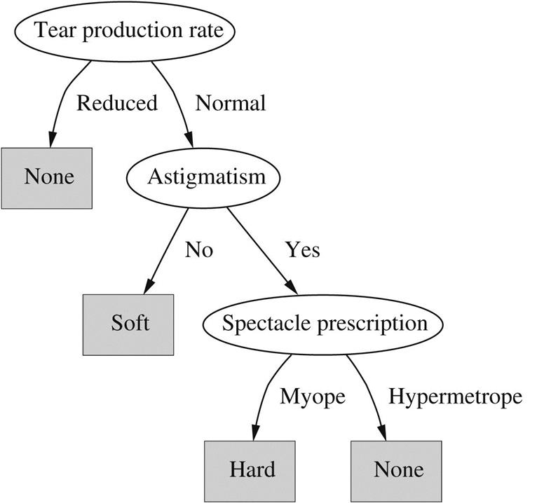
Fig. 1.2 shows a structural description for the contact lens data in the form of a decision tree, which for many purposes is a more concise and perspicuous representation of the rules and has the advantage that it can be visualized more easily. (However, this decision tree—in contrast to the rule set given in Fig. 1.1—classifies two examples incorrectly.) The tree calls first for a test on tear production rate, and the first two branches correspond to the two possible outcomes. If tear production rate is reduced (the left branch), the outcome is none. If it is normal (the right branch), a second test is made, this time on astigmatism. Eventually, whatever the outcome of the tests, a leaf of the tree is reached that dictates the contact lens recommendation for that case. The question of what is the most natural and easily understood format for the output from a machine learning scheme is one that we will return to in Chapter 3, Output: knowledge representation.
Irises: A Classic Numeric Dataset
The iris dataset, which dates back to seminal work by the eminent statistician R.A. Fisher in the mid-1930s and is arguably the most famous dataset used in machine learning, contains 50 examples each of three types of plant: Iris setosa, Iris versicolor, and Iris virginica. It is excerpted in Table 1.4. There are four attributes: sepal length, sepal width, petal length, and petal width (all measured in centimeters). Unlike previous datasets, all attributes have values that are numeric.
Table 1.4
| Sepal Length | Sepal Width | Petal Length | Petal Width | Type | |
| 1 | 5.1 | 3.5 | 1.4 | 0.2 | Iris setosa |
| 2 | 4.9 | 3.0 | 1.4 | 0.2 | I. setosa |
| 3 | 4.7 | 3.2 | 1.3 | 0.2 | I. setosa |
| 4 | 4.6 | 3.1 | 1.5 | 0.2 | I. setosa |
| 5 | 5.0 | 3.6 | 1.4 | 0.2 | I. setosa |
| … | |||||
| 51 | 7.0 | 3.2 | 4.7 | 1.4 | Iris versicolor |
| 52 | 6.4 | 3.2 | 4.5 | 1.5 | I. versicolor |
| 53 | 6.9 | 3.1 | 4.9 | 1.5 | I. versicolor |
| 54 | 5.5 | 2.3 | 4.0 | 1.3 | I. versicolor |
| 55 | 6.5 | 2.8 | 4.6 | 1.5 | I. versicolor |
| … | |||||
| 101 | 6.3 | 3.3 | 6.0 | 2.5 | Iris virginica |
| 102 | 5.8 | 2.7 | 5.1 | 1.9 | I. virginica |
| 103 | 7.1 | 3.0 | 5.9 | 2.1 | I. virginica |
| 104 | 6.3 | 2.9 | 5.6 | 1.8 | I. virginica |
| 105 | 6.5 | 3.0 | 5.8 | 2.2 | I. virginica |
| … |

The following set of rules might be learned from this dataset:
If petal-length < 2.45 then Iris-setosa
If sepal-width < 2.10 then Iris-versicolor
If sepal-width < 2.45 and petal-length < 4.55 then Iris-versicolor
If sepal-width < 2.95 and petal-width < 1.35 then Iris-versicolor
If petal-length ≥2.45 and petal-length < 4.45 then Iris-versicolor
If sepal-length ≥5.85 and petal-length < 4.75 then Iris-versicolor
If sepal-width < 2.55 and petal-length < 4.95 and petal-width < 1.55 then Iris-versicolor
If petal-length ≥2.45 and petal-length < 4.95 and petal-width < 1.55 then Iris-versicolor
If sepal-length ≥6.55 and petal-length < 5.05 then Iris-versicolor
If sepal-width < 2.75 and petal-width < 1.65 and sepal-length < 6.05 then Iris-versicolor
If sepal-length ≥5.85 and sepal-length < 5.95 and petal-length < 4.85 then Iris-versicolor
If petal-length ≥5.15 then Iris-virginica
If petal-width ≥1.85 then Iris-virginica
If petal-width ≥1.75 and sepal-width < 3.05 then Iris-virginica
If petal-length ≥4.95 and petal-width < 1.55 then Iris-virginica
These rules are very cumbersome, and we will see in Chapter 3, Output: knowledge representation, how more compact rules can be expressed that convey the same information.
CPU Performance: Introducing Numeric Prediction
Although the iris dataset involves numeric attributes, the outcome—the type of iris—is a category, not a numeric value. Table 1.5 shows some data for which both the outcome and the attributes are numeric. It concerns the relative performance of computer processing power on the basis of a number of relevant attributes: each row represents 1 of 209 different computer configurations.
Table 1.5
| Cycle Time (ns) | Main Memory (Kb) | Cache(KB) | Channels | Performance | |||
| Min | Max | Min | Max | ||||
| MYCT | MMIN | MMAX | CACH | CHMIN | CHMAX | PRP | |
| 1 | 125 | 256 | 6000 | 256 | 16 | 128 | 198 |
| 2 | 29 | 8000 | 32,000 | 32 | 8 | 32 | 269 |
| 3 | 29 | 8000 | 32,000 | 32 | 8 | 32 | 220 |
| 4 | 29 | 8000 | 32,000 | 32 | 8 | 32 | 172 |
| 5 | 29 | 8000 | 16,000 | 32 | 8 | 16 | 132 |
| … | |||||||
| 207 | 125 | 2000 | 8000 | 0 | 2 | 14 | 52 |
| 208 | 480 | 512 | 8000 | 32 | 0 | 0 | 67 |
| 209 | 480 | 1000 | 4000 | 0 | 0 | 0 | 45 |

The classic way of dealing with continuous prediction is to write the outcome as a linear sum of the attribute values with appropriate weights, e.g.,
(The abbreviated variable names are given in the second row of the table.) This is called a linear regression equation, and the process of determining the weights is called linear regression, a well-known procedure in statistics that we will review in Chapter 4, Algorithms: the basic methods. The basic regression method is incapable of discovering nonlinear relationships, but variants exist—we encounter them later in this book. In Chapter 3, Output: knowledge representation, we will examine other representations that can be used for predicting numeric quantities.
In the iris and central processing unit (CPU) performance data, all the attributes have numeric values. Practical situations frequently present a mixture of numeric and nonnumeric attributes.
Labor Negotiations: A More Realistic Example
The labor negotiations dataset in Table 1.6 summarizes the outcome of Canadian labor contract negotiations in 1987 and 1988. It includes all collective agreements reached in the business and personal services sector for organizations with at least 500 members (teachers, nurses, university staff, police, etc.). Each case concerns one contract, and the outcome is whether the contract is deemed acceptable or unacceptable. The acceptable contracts are ones in which agreements were accepted by both labor and management. The unacceptable ones are either known offers that fell through because one party would not accept them or acceptable contracts that had been significantly perturbed to the extent that, in the view of experts, they would not have been accepted.
Table 1.6
| Attribute | Type | 1 | 2 | 3 | … | 40 |
| Duration | (Number of years) | 1 | 2 | 3 | 2 | |
| Wage increase 1st year | Percentage | 2% | 4% | 4.3% | 4.5 | |
| Wage increase 2nd year | Percentage | ? | 5% | 4.4% | 4.0 | |
| Wage increase 3rd year | Percentage | ? | ? | ? | ? | |
| Cost of living adjustment | {None, tcf, tc} | None | Tcf | ? | None | |
| Working hours per week | (Number of hours) | 28 | 35 | 38 | 40 | |
| Pension | {None, ret-allw, empl-cntr} | None | ? | ? | ? | |
| Standby pay | Percentage | ? | 13% | ? | ? | |
| Shift-work supplement | Percentage | ? | 5% | 4% | 4 | |
| Education allowance | {Yes, no} | Yes | ? | ? | ? | |
| Statutory holidays | (Number of days) | 11 | 15 | 12 | 12 | |
| Vacation | {Below-avg, avg, gen} | Avg | Gen | Gen | Avg | |
| Long-term disability assistance | {Yes, no} | No | ? | ? | Yes | |
| Dental plan contribution | {None, half, full} | None | ? | Full | Full | |
| Bereavement assistance | {Yes, no} | No | ? | ? | Yes | |
| Health-plan contribution | {None, half, full} | None | ? | Full | Half | |
| Acceptability of contract | {Good, bad} | Bad | Good | Good | Good |

There are 40 examples in the dataset (plus another 17 that are normally reserved for test purposes). Unlike the other tables here, Table 1.6 presents the examples as columns rather than as rows; otherwise, it would have to be stretched over several pages. Many of the values are unknown or missing, as indicated by question marks.
This is a much more realistic dataset than the others we have seen. It contains many missing values, and it seems unlikely that an exact classification can be obtained.
Fig. 1.3 shows two decision trees that represent the dataset. Fig. 1.3A is simple and approximate: it doesn’t represent the data exactly. For example, it will predict bad for some contracts that are actually marked good. But it does make intuitive sense: a contract is bad (for the employee!) if the wage increase in the first year is too small (less than 2.5%). If the first-year wage increase is larger than this, it is good if there are lots of statutory holidays (more than 10 days). Even if there are fewer statutory holidays, it is good if the first-year wage increase is large enough (more than 4%).

Fig. 1.3B is a more complex decision tree that represents the same dataset. Take a detailed look down the left branch. At first sight it doesn’t seem to make sense intuitively that, if the working hours exceed 36, a contract is bad if there is no health-plan contribution or a full health-plan contribution but is good if there is a half health-plan contribution. It is certainly reasonable that the health-plan contribution plays a role in the decision, but it seems anomalous that half is good and both full and none are bad. However, on reflection this could make sense after all, because “good” contracts are ones that have been accepted by both parties: labor and management. Perhaps this structure reflects compromises that had to be made to get agreement. This kind of detailed reasoning about what parts of decision trees mean is a good way of getting to know your data and think about the underlying problem.
In fact, Fig. 1.3B is a more accurate representation of the training dataset than Fig. 1.3A. But it is not necessarily a more accurate representation of the underlying concept of good versus bad contracts. Although it is more accurate on the data that was used to train the classifier, it may perform less well on an independent set of test data. It may be “overfitted” to the training data—following it too slavishly. The tree in Fig. 1.3A is obtained from the one in Fig. 1.3B by a process of pruning, which we will learn more about in Chapter 6, Trees and rules.
Soybean Classification: A Classic Machine Learning Success
An often quoted early success story in the application of machine learning to practical problems is the identification of rules for diagnosing soybean diseases. The data is taken from questionnaires describing plant diseases. There are about 680 examples, each representing a diseased plant. Plants were measured on 35 attributes, each one having a small set of possible values. Examples are labeled with the diagnosis of an expert in plant biology: there are 19 disease categories altogether—horrible-sounding diseases such as diaporthe stem canker, rhizoctonia root rot, and bacterial blight, to mention just a few.
Table 1.7 gives the attributes, the number of different values that each can have, and a sample record for one particular plant. The attributes are placed into different categories just to make them easier to read.
Table 1.7
| Attribute | Number of Values | Sample Value | |
| Environment | Time of occurrence | 7 | July |
| Precipitation | 3 | Above normal | |
| Temperature | 3 | Normal | |
| Cropping history | 4 | Same as last year | |
| Hail damage | 2 | Yes | |
| Damaged area | 4 | Scattered | |
| Severity | 3 | Severe | |
| Plant height | 2 | Normal | |
| Plant growth | 2 | Abnormal | |
| Seed treatment | 3 | Fungicide | |
| Germination | 3 | Less than 80% | |
| Seed | Condition | 2 | Normal |
| Mold growth | 2 | Absent | |
| Discoloration | 2 | Absent | |
| Size | 2 | Normal | |
| Shriveling | 2 | Absent | |
| Fruit | Condition of fruit pods | 3 | Normal |
| Fruit spots | 5 | – | |
| Leaves | Condition | 2 | Abnormal |
| Leaf spot size | 3 | – | |
| Yellow leaf spot halo | 3 | Absent | |
| Leaf spot margins | 3 | – | |
| Shredding | 2 | Absent | |
| Leaf malformation | 2 | Absent | |
| Leaf mildew growth | 3 | Absent | |
| Stem | Condition | 2 | Abnormal |
| Stem lodging | 2 | Yes | |
| Stem cankers | 4 | Above soil line | |
| Canker lesion color | 3 | – | |
| Fruiting bodies on stems | 2 | Present | |
| External decay of stem | 3 | Firm and dry | |
| Mycelium on stem | 2 | Absent | |
| Internal discoloration | 3 | None | |
| Sclerotia | 2 | Absent | |
| Roots | Condition | 3 | Normal |
| Diagnosis | 19 | Diaporthe stem canker |

Here are two example rules, learned from this data:
If leaf condition=normal and
stem condition=abnormal and
stem cankers=below soil line and
canker lesion color=brown
then
diagnosis is rhizoctonia root rot
If leaf malformation=absent and
stem condition=abnormal and
stem cankers=below soil line and
canker lesion color=brown
then
diagnosis is rhizoctonia root rot
These rules nicely illustrate the potential role of prior knowledge—often called domain knowledge—in machine learning, for in fact the only difference between the two descriptions is leaf condition is normal versus leaf malformation is absent. Now, in this domain, if the leaf condition is normal then leaf malformation is necessarily absent, so one of these conditions happens to be a special case of the other. Thus if the first rule is true, the second is necessarily true as well. The only time the second rule comes into play is when leaf malformation is absent but leaf condition is not normal, i.e., when something other than malformation is wrong with the leaf. This is certainly not apparent from a casual reading of the rules.
Research on this problem in the late 1970s found that these diagnostic rules could be generated by a machine learning algorithm, along with rules for every other disease category, from about 300 training examples. These training examples were carefully selected from the corpus of cases as being quite different from one another—“far apart” in the example space. At the same time, the plant pathologist who had produced the diagnoses was interviewed, and his expertise was translated into diagnostic rules. Surprisingly, the computer-generated rules outperformed the expert-derived rules on the remaining test examples. They gave the correct disease top ranking 97.5% of the time compared with only 72% for the expert-derived rules. Furthermore, not only did the learning algorithm find rules that outperformed those of the expert collaborator, but the same expert was so impressed that he allegedly adopted the discovered rules in place of his own!
1.3 Fielded Applications
The examples that we opened with are speculative research projects, not production systems. And most of the illustrations above are toy problems: they are deliberately chosen to be small so that we can use them to work through algorithms later in the book. Where’s the beef? Here are some applications of machine learning that have actually been put into use.
Being fielded applications, the illustrations that follow tend to stress the use of learning in performance situations, in which the emphasis is on the ability to perform well on new examples. This book also describes the use of learning systems to gain knowledge from decision structures that are inferred from the data. We believe that this is as important a use of the technology as making high-performance predictions. Still, it will tend to be underrepresented in fielded applications because when learning techniques are used to gain insight, the result is not normally a system that is put to work as an application in its own right. Nevertheless, in three of the examples below, the fact that the decision structure is comprehensible is a key feature in the successful adoption of the application.
Web Mining
Mining information on the World Wide Web is a huge application area. Search engine companies examine the hyperlinks in web pages to come up with a measure of “prestige” for each web page and website. Dictionaries define prestige as “high standing achieved through success or influence.” A metric called PageRank, introduced by the founders of Google and used in various guises by other search engine developers too, attempts to measure the standing of a web page. The more pages that link to your website, the higher its prestige. And prestige is greater if the pages that link in have high prestige themselves. The definition sounds circular, but it can be made to work. Search engines use PageRank (among other things) to sort web pages into order before displaying the result of your search.
Another way in which search engines tackle the problem of how to rank web pages is to use machine learning based on a training set of example queries—documents that contain the terms in the query and human judgments about how relevant the documents are to that query. Then a learning algorithm analyzes this training data and comes up with a way to predict the relevance judgment for any document and query. For each document a set of feature values is calculated that depend on the query term—e.g., whether it occurs in the title tag, whether it occurs in the document’s URL, how often it occurs in the document itself, and how often it appears in the anchor text of hyperlinks that point to this document. For multiterm queries, features include how often two different terms appear close together in the document, and so on. There are many possible features: typical algorithms for learning ranks use hundreds or thousands of them.
Search engines mine the content of the Web. They also mine the content of your queries—the terms you search for—to select advertisements that you might be interested in. They have a strong incentive to do this accurately, because they only get paid by advertisers when users click on their links. Search engine companies mine your very clicks, because knowledge of which results you click on can be used to improve the search next time. Online booksellers mine the purchasing database to come up with recommendations such as “users who bought this book also bought these ones”; again they have a strong incentive to present you with compelling, personalized choices. Movie sites recommend movies based on your previous choices and other people’s choices: they win if they make recommendations that keep customers coming back to their website.
And then there are social networks and other personal data. We live in the age of selfrevelation: people share their innermost thoughts in blogs and tweets, their photographs, their music and movie tastes, their opinions of books, software, gadgets, and hotels, their social life. They may believe they are doing this anonymously, or pseudonymously, but often they are incorrect (see Section 1.6). There is huge commercial interest in making money by mining the Web.
Decisions Involving Judgment
When you apply for a loan, you have to fill out a questionnaire asking for relevant financial and personal information. This information is used by the loan company as the basis for its decision as to whether to lend you money. Such decisions are often made in two stages: first, statistical methods are used to determine clear “accept” and “reject” cases. The remaining borderline cases are more difficult and call for human judgment. For example, one loan company uses a statistical decision procedure to calculate a numeric parameter based on the information supplied in the questionnaire. Applicants are accepted if this parameter exceeds a preset threshold and rejected if it falls below a second threshold. This accounts for 90% of cases, and the remaining 10% are referred to loan officers for a decision. On examining historical data on whether applicants did indeed repay their loans, however, it turned out that half of the borderline applicants who were granted loans actually defaulted. Although it would be tempting simply to deny credit to borderline customers, credit industry professionals pointed out that if only their repayment future could be reliably determined it is precisely these customers whose business should be wooed; they tend to be active customers of a credit institution because their finances remain in a chronically volatile condition. A suitable compromise must be reached between the viewpoint of a company accountant, who dislikes bad debt, and that of a sales executive, who dislikes turning business away.
Enter machine learning. The input was 1000 training examples of borderline cases for which a loan had been made that specified whether the borrower had finally paid off or defaulted. For each training example, about 20 attributes were extracted from the questionnaire, such as age, years with current employer, years at current address, years with the bank, and other credit cards possessed. A machine learning procedure was used to produce a small set of classification rules that made correct predictions on two-thirds of the borderline cases in an independently chosen test set. Not only did these rules improve the success rate of the loan decisions, but the company also found them attractive because they could be used to explain to applicants the reasons behind the decision. Although the project was an exploratory one that took only a small development effort, the loan company was apparently so pleased with the result that the rules were put into use immediately.
Screening Images
Since the early days of satellite technology, environmental scientists have been trying to detect oil slicks from satellite images to give early warning of ecological disasters and deter illegal dumping. Radar satellites provide an opportunity for monitoring coastal waters day and night, regardless of weather conditions. Oil slicks appear as dark regions in the image whose size and shape evolve depending on weather and sea conditions. However, other look-alike dark regions can be caused by local weather conditions such as high wind. Detecting oil slicks is an expensive manual process requiring highly trained personnel who assess each region in the image.
A hazard detection system has been developed to screen images for subsequent manual processing. Intended to be marketed worldwide to a wide variety of users—government agencies and companies—with different objectives, applications, and geographical areas, it needs to be highly customizable to individual circumstances. Machine learning allows the system to be trained on examples of spills and nonspills supplied by the user and lets the user control the tradeoff between undetected spills and false alarms. Unlike other machine learning applications, which generate a classifier that is then deployed in the field, here it is the learning scheme itself that will be deployed.
The input is a set of raw pixel images from a radar satellite, and the output is a much smaller set of images with putative oil slicks marked by a colored border. First, standard image-processing operations are applied to normalize the image. Then, suspicious dark regions are identified. Several dozen attributes are extracted from each region, characterizing its size, shape, area, intensity, sharpness, and jaggedness of the boundaries, proximity to other regions, and information about the background in the vicinity of the region. Finally, standard learning techniques are applied to the resulting attribute vectors. (An alternative, omitting explicit feature extraction steps, would be to use the deep learning approach discussed in Chapter 10, Deep learning).
Several interesting problems were encountered. One is the scarcity of training data. Oil slicks are (fortunately) very rare, and manual classification is extremely costly. Another is the unbalanced nature of the problem: of the many dark regions in the training data, only a very small fraction are actual oil slicks. A third is that the examples group naturally into batches, with regions drawn from each image forming a single batch, and background characteristics vary from one batch to another. Finally, the performance task is to serve as a filter, and the user must be provided with a convenient means of varying the false-alarm rate.
Load Forecasting
In the electricity supply industry, it is important to determine future demand for power as far in advance as possible. If accurate estimates can be made for the maximum and minimum load for each hour, day, month, season, and year, utility companies can make significant economies in areas such as setting the operating reserve, maintenance scheduling, and fuel inventory management.
An automated load-forecasting assistant has been operating at a major utility supplier for more than a decade to generate hourly forecasts 2 days in advance. The first step was to use data collected over the previous 15 years to create a sophisticated load model manually. This model had three components: base load for the year, load periodicity over the year, and effect of holidays. To normalize for the base load, the data for each previous year was standardized by subtracting the average load for that year from each hourly reading and dividing by the standard deviation over the year. Electric load shows periodicity at three fundamental frequencies: diurnal, where usage has an early morning minimum and midday and afternoon maxima; weekly, where demand is lower at weekends; and seasonal, where increased demand during winter and summer for heating and cooling, respectively, creates a yearly cycle. Major holidays such as Thanksgiving, Christmas, and New Year’s Day show significant variation from the normal load and are each modeled separately by averaging hourly loads for that day over the past 15 years. Minor official holidays, such as Columbus Day, are lumped together as school holidays and treated as an offset to the normal diurnal pattern. All of these effects are incorporated by reconstructing a year’s load as a sequence of typical days, fitting the holidays in their correct position, and denormalizing the load to account for overall growth.
Thus far, the load model is a static one, constructed manually from historical data, and implicitly assumes “normal” climatic conditions over the year. The final step was to take weather conditions into account by locating the previous day most similar to the current circumstances and using the historical information from that day as a predictor. The prediction is treated as an additive correction to the static load model. To guard against outliers, the eight most similar days are located and their additive corrections averaged. A database was constructed of temperature, humidity, wind speed, and cloud cover at three local weather centers for each hour of the 15-year historical record, along with the difference between the actual load and that predicted by the static model. A linear regression analysis was performed to determine the relative effects of these observations on load, and the coefficients were applied to weight the distance function used to locate the most similar days.
The resulting system yielded the same performance as trained human forecasters but was far quicker—taking seconds rather than hours to generate a daily forecast. Human operators can analyze the forecast’s sensitivity to simulated changes in weather and bring up for examination the “most similar” days that the system used for weather adjustment.
Diagnosis
Diagnosis is one of the principal application areas of expert systems. Although the hand-crafted rules used in expert systems often perform well, machine learning can be useful in situations in which producing rules manually is too labor intensive.
Preventative maintenance of electromechanical devices such as motors and generators can forestall failures that disrupt industrial processes. Technicians regularly inspect each device, measuring vibrations at various points to determine whether the device needs servicing. Typical faults include shaft misalignment, mechanical loosening, faulty bearings, and unbalanced pumps. A particular chemical plant uses more than 1000 different devices, ranging from small pumps to very large turbo-alternators, which used to be diagnosed by a human expert with 20 years of experience. Faults are identified by measuring vibrations at different places on the device’s mounting and using Fourier analysis to check the energy present in three different directions at each harmonic of the basic rotation speed. This information, which is very noisy because of limitations in the measurement and recording procedure, can be studied by the expert to arrive at a diagnosis. Although handcrafted expert system rules had been elicited for some situations, the elicitation process would have to be repeated several times for different types of machinery; so a learning approach was investigated.
Six hundred faults, each comprising a set of measurements along with the expert’s diagnosis, were available, representing 20 years of experience. About half were unsatisfactory for various reasons and had to be discarded; the remainder were used as training examples. The goal was not to determine whether or not a fault existed, but to diagnose the kind of fault, given that one was there. Thus there was no need to include fault-free cases in the training set. The measured attributes were rather low level and had to be augmented by intermediate concepts, i.e., functions of basic attributes, which were defined in consultation with the expert and embodied some causal domain knowledge. The derived attributes were run through an induction algorithm to produce a set of diagnostic rules. Initially, the expert was not satisfied with the rules because he could not relate them to his own knowledge and experience. For him, mere statistical evidence was not, by itself, an adequate explanation. Further background knowledge had to be used before satisfactory rules were generated. Although the resulting rules were quite complex, the expert liked them because he could justify them in light of his mechanical knowledge. He was pleased that a third of the rules coincided with ones he used himself and was delighted to gain new insight from some of the others.
Performance tests indicated that the learned rules were slightly superior to the handcrafted ones that had previously been elicited from the expert, and this result was confirmed by subsequent use in the chemical factory. It is interesting to note, however, that the system was put into use not because of its good performance but because the domain expert approved of the rules that had been learned.
Marketing and Sales
Some of the most active applications of data mining have been in the area of marketing and sales. These are domains in which companies possess massive volumes of precisely recorded data, data that is potentially extremely valuable. In these applications, predictions themselves are the chief interest: the structure of how decisions are made is often completely irrelevant.
We have already mentioned the problem of fickle customer loyalty and the challenge of detecting customers who are likely to defect so that they can be wooed back into the fold by giving them special treatment. Banks were early adopters of data mining technology because of their successes in the use of machine learning for credit assessment. Data mining is now being used to reduce customer attrition by detecting changes in individual banking patterns that may herald a change of bank, or even life changes—such as a move to another city—that could result in a different bank being chosen. It may reveal, e.g., a group of customers with above-average attrition rate who do most of their banking by phone after hours when telephone response is slow. Data mining may determine groups for whom new services are appropriate, such as a cluster of profitable, reliable customers who rarely get cash advances from their credit card except in November and December, when they are prepared to pay exorbitant interest rates to see them through the holiday season. In another domain, cellular phone companies fight churn by detecting patterns of behavior that could benefit from new services, and then advertise such services to retain their customer base. Incentives provided specifically to retain existing customers can be expensive, and successful data mining allows them to be precisely targeted to those customers who are likely to yield maximum benefit.
Market basket analysis is the use of association techniques to find groups of items that tend to occur together in transactions, e.g., supermarket checkout data. For many retailers this is the only source of sales information that is available for data mining. For example, automated analysis of checkout data may uncover the fact that customers who buy beer also buy chips, a discovery that could be significant from the supermarket operator’s point of view (although rather an obvious one that probably does not need a data mining exercise to discover). Or it may come up with the fact that on Thursdays, customers often purchase diapers and beer together, an initially surprising result that, on reflection, makes some sense as young parents stock up for a weekend at home. Such information could be used for many purposes: planning store layouts, limiting special discounts to just one of a set of items that tend to be purchased together, offering coupons for a matching product when one of them is sold alone, and so on.
There is enormous added value in being able to identify individual customer’s sales histories. Discount or “loyalty” cards let retailers identify all the purchases that each individual customer makes. This personal data is far more valuable than the cash value of the discount. Identification of individual customers not only allows historical analysis of purchasing patterns but also permits precisely targeted special offers to be mailed out to prospective customers—or perhaps personalized coupons can be printed in real time at the checkout for use during the next grocery run. Supermarkets want you to feel that although we may live in a world of inexorably rising prices, they don’t increase so much for you because the bargains offered by personalized coupons make it attractive for you to stock up on things that you wouldn’t normally have bought.
Direct marketing is another popular domain for data mining. Bulk-mail promotional offers are expensive, and have a low—but highly profitable—response rate. Anything that helps focus promotions, achieving the same or nearly the same response from a smaller sample, is valuable. Commercially available databases containing demographic information that characterize neighborhoods based on ZIP codes can be correlated with information on existing customers to predict what kind of people might buy which items. This model can be trialed on information gained in response to an initial mailout, where people send back a response card or call an 800 number for more information, to predict likely future customers. Unlike shopping-mall retailers, direct mail companies have complete purchasing histories for each individual customer and can use data mining to determine those likely to respond to special offers. Targeted campaigns save money—and reduce annoyance—by directing offers only to those likely to want the product.
Other Applications
There are countless other applications of machine learning. We briefly mention a few more areas to illustrate the breadth of what has been done.
Sophisticated manufacturing processes often involve tweaking control parameters. Separating crude oil from natural gas is an essential prerequisite to oil refinement, and controlling the separation process is a tricky job. British Petroleum used machine learning to create rules for setting the parameters. Setting parameters using these rules takes just 10 minutes, whereas human experts take more than a day. Westinghouse faced problems in their process for manufacturing nuclear fuel pellets and used machine learning to create rules to control the process. This was reported to save them more than $10 million per year (in 1984). The Tennessee printing company R.R. Donnelly applied the same idea to control rotogravure printing presses to reduce artifacts caused by inappropriate parameter settings, reducing the number of artifacts from more than 500 each year to less than 30.
In the realm of customer support and service, we have already described adjudicating loans, and marketing and sales applications. Another example arises when a customer reports a telephone problem and the company must decide what kind of technician to assign to the job. An expert system developed by Bell Atlantic in 1991 to make this decision was replaced in 1999 by a set of rules learned using machine learning, which saved more than $10 million per year by making fewer incorrect decisions.
There are many scientific applications. In biology, machine learning is used to help identify the thousands of genes within each new genome. In biomedicine, it is used to predict drug activity by analyzing not just the chemical properties of drugs but also their three-dimensional structure. This accelerates drug discovery and reduces its cost. In astronomy, machine learning has been used to develop a fully automatic cataloguing system for celestial objects that are too faint to be seen by visual inspection. In chemistry, it has been used to predict the structure of certain organic compounds from magnetic resonance spectra. In all these applications, machine learning techniques have attained levels of performance—or should we say skill?—that rival or surpass human experts.
Automation is especially welcome in situations involving continuous monitoring, a job that is time consuming and exceptionally tedious for humans. Ecological applications include the oil spill monitoring described earlier. Some other applications are rather less consequential—e.g., machine learning is being used to predict preferences for TV programs based on past choices and advise viewers about the available channels. Still others may save lives. Intensive care patients may be monitored to detect changes in variables that cannot be explained by circadian rhythm, medication, and so on, raising an alarm when appropriate. Finally, in a world that relies on vulnerable networked computer systems and is increasingly concerned about cybersecurity, machine learning is used to detect intrusion by recognizing unusual patterns of operation.
1.4 The Data Mining Process
This book is about machine learning techniques for data mining: the technical core of practical data mining applications. Successful implementation of these techniques in a business context requires an understanding of important aspects that we do not—and cannot—cover in this book.
Fig. 1.4 shows the life cycle of a data mining project, as defined by the CRISP-DM reference model. Before data mining can be applied, you need to understand what you want to achieve by implementing it. This is the “business understanding” phase: investigating the business objectives and requirements, deciding whether data mining can be applied to meet them, and determining what kind of data can be collected to build a deployable model. In the next phase, “data understanding,” an initial dataset is established and studied to see whether it is suitable for further processing. If the data quality is poor, it may be necessary to collect new data based on more stringent criteria. Insights into the data that are gained at this stage may also trigger reconsideration of the business context—perhaps the objective of applying data mining needs to be reviewed?

The next three steps—data preparation, modeling, and evaluation—are what this book deals with. Preparation involves preprocessing the raw data so that machine learning algorithms can produce a model—ideally, a structural description of the information that is implicit in the data. Preprocessing may include model building activities as well, because many preprocessing tools build an internal model of the data to transform it. In fact, data preparation and modeling usually go hand in hand. It is almost always necessary to iterate: results obtained during modeling provide new insights that affect the choice of preprocessing techniques.
The next phase in any successful application of data mining—and its importance cannot be overstated!—is evaluation. Do the structural descriptions inferred from the data have any predictive value, or do they simply reflect spurious regularities? This book explains many techniques for estimating the predictive performance of models built by machine learning. If the evaluation step shows that the model is poor, you may need to reconsider the entire project and return to the business understanding step to identify more fruitful business objectives or avenues for data collection. If, on the other hand, the model’s accuracy is sufficiently high, the next step is to deploy it in practice. This normally involves integrating it into a larger software system, so the model needs to be handed over to the project’s software engineers. This is the stage where the implementation details of the modeling techniques matter. For example, to slot the model into the software system it may be necessary to reimplement it in a different programming language.
1.5 Machine Learning and Statistics
What’s the difference between machine learning and statistics? Cynics, looking wryly at the explosion of commercial interest (and hype) in this area, equate data mining to statistics plus marketing. In truth, you should not look for a dividing line between machine learning and statistics because there is a continuum—and a multidimensional one at that—of data analysis techniques. Some derive from the skills taught in standard statistics courses, and others are more closely associated with the kind of machine learning that has arisen out of computer science. Historically, the two sides have had rather different traditions. If forced to point to a single difference of emphasis, it might be that statistics has been more concerned with testing hypotheses, whereas machine learning has been more concerned with formulating the process of generalization as a search through possible hypotheses. But this is a gross oversimplification: statistics is far more than just hypothesis-testing, and many machine learning techniques do not involve any searching at all.
In the past, very similar schemes have developed in parallel in machine learning and statistics. One is decision tree induction. Four statisticians at Californian universities published a book on Classification and regression trees in the mid-1980s, and throughout the 1970s and early 1980s a prominent Australian machine learning researcher, J. Ross Quinlan, was developing a system for inferring classification trees from examples. These two independent projects produced quite similar schemes for generating trees from examples, and the researchers only became aware of one another’s work much later. A second area where similar methods have arisen involves the use of nearest-neighbor methods for classification. These are standard statistical techniques that have been extensively adapted by machine learning researchers, both to improve classification performance and to make the procedure more efficient computationally. We will examine both decision tree induction and nearest-neighbor methods in Chapter 4, Algorithms: the basic methods.
But now the two perspectives have converged. The techniques we will examine in this book incorporate a great deal of statistical thinking. Right from the beginning, when constructing and refining the initial example set, standard statistical methods apply: visualization of data, selection of attributes, discarding outliers, and so on. Many learning algorithms use statistical tests when constructing rules or trees and for correcting models that are “overfitted” in that they depend too strongly on the details of the particular examples used to produce them (we have already seen an example of this in the two decision trees of Fig. 1.3 for the labor negotiations problem). Statistical tests are used to validate machine learning models and to evaluate machine learning algorithms. In our study of practical techniques for data mining, we will learn a great deal about statistics.
1.6 Generalization as Search
One way of visualizing the problem of learning—and one that distinguishes it from statistical approaches—is to imagine a search through a space of possible concept descriptions for one that fits the data. Although the idea of generalization as search is a powerful conceptual tool for thinking about machine learning, it is not essential for understanding the practical schemes described in this book. That is why this section is marked optional, as indicated by the gray bar in the margin.
Suppose, for definiteness, that concept descriptions—the result of learning—are expressed as rules such as the ones given for the weather problem in Section 1.2 (although other concept description languages would do just as well). Suppose that we list all possible sets of rules and then look for ones that satisfy a given set of examples. A big job? Yes. An infinite job? At first glance it seems so because there is no limit to the number of rules there might be. But actually the number of possible rule sets is finite. Note first that each individual rule is no greater than a fixed maximum size, with at most one term for each attribute: for the weather data of Table 1.2 this involves four terms in all. Because the number of possible rules is finite, the number of possible rule sets is finite too, although extremely large. However, we’d hardly be interested in sets that contained a very large number of rules. In fact, we’d hardly be interested in sets that had more rules than there are examples because it is difficult to imagine needing more than one rule for each example. So if we were to restrict consideration to rule sets smaller than that, the problem would be substantially reduced, although still very large.
The threat of an infinite number of possible concept descriptions seems more serious for the second version of the weather problem in Table 1.3 because these rules contain numbers. If they are real numbers, you can’t enumerate them, even in principle. However, on reflection the problem again disappears because the numbers really just represent breakpoints in the numeric values that appear in the examples. For instance, consider the temperature attribute in Table 1.3. It involves the numbers 64, 65, 68, 69, 70, 71, 72, 75, 80, 81, 83, and 85—12 different numbers. There are 13 possible places in which we might want to put a breakpoint for a rule involving temperature. The problem isn’t infinite after all.
So the process of generalization with rule sets can be regarded as a search through an enormous, but finite, search space. In principle, the problem can be solved by enumerating descriptions and striking out those that do not fit the examples presented—assuming there is no noise in the examples, and the description language is sufficiently expressive. A positive example eliminates all descriptions that it does not match, and a negative one eliminates those it does match. With each example the set of remaining descriptions shrinks (or stays the same). If only one is left, it is the target description—the target concept.
If several descriptions are left, they may still be used to classify unknown objects. An unknown object that matches all remaining descriptions should be classified as matching the target; if it fails to match any description it should be classified as being outside the target concept. Only when it matches some descriptions but not others is there ambiguity. In this case if the classification of the unknown object were revealed, it would cause the set of remaining descriptions to shrink because rule sets that classified the object the wrong way would be rejected.
Enumerating the Concept Space
Regarding it as search is a good way of looking at the learning process. However, the search space, although finite, is extremely big, and it is generally quite impractical to enumerate all possible descriptions and then see which ones fit. In the weather problem there are 4×4×3×3×2=288 possibilities for each rule. There are four possibilities for the outlook attribute: sunny, overcast, rainy, or it may not participate in the rule at all. Similarly, there are four for temperature, three for windy and humidity, and two for the class. If we restrict the rule set to contain no more than 14 rules (because there are 14 examples in the training set), there are around 2.7×1034 possible different rule sets. That’s a lot to enumerate, especially for such a patently trivial problem.
Although there are ways of making the enumeration procedure more feasible, a serious problem remains: in practice, it is rare for the process to converge on a unique acceptable description. Either many descriptions are still in the running after the examples are processed or the descriptors are all eliminated. The first case arises when the examples are not sufficiently comprehensive to eliminate all possible descriptions except for the “correct” one. In practice, people often want a single “best” description, and it is necessary to apply some other criteria to select the best one from the set of remaining descriptions. The second problem arises either because the description language is not expressive enough to capture the actual concept or because of noise in the examples. If an example comes in with the “wrong” classification due to an error in some of the attribute values or in the class that is assigned to it, this will likely eliminate the correct description from the space. The result is that the set of remaining descriptions becomes empty. This situation is very likely to happen if the examples contain any noise at all, which inevitably they do except in artificial situations.
Another way of looking at generalization as search is to imagine it not as a process of enumerating descriptions and striking out those that don’t apply but as a kind of hill-climbing in description space to find the description that best matches the set of examples according to some prespecified matching criterion. This is the way that most practical machine learning methods work. However, it is often impractical to search the whole space exhaustively; many practical algorithms involve heuristic search and cannot guarantee to find the optimal description.
Bias
Viewing generalization as a search in a space of possible concepts makes it clear that the most important decisions in a machine learning system are:
• the concept description language;
• the order in which the space is searched;
• the way that overfitting to the particular training data is avoided.
These three properties are generally referred to as the bias of the search and are called language bias, search bias, and overfitting-avoidance bias. You bias the learning scheme by choosing a language in which to express concepts, by searching in a particular way for an acceptable description, and by deciding when the concept has become so complex that it needs to be simplified.
Language bias
The most important question for language bias is whether the concept description language is universal or whether it imposes constraints on what concepts can be learned. If you consider the set of all possible examples, a concept is really just a division of it into subsets. In the weather example, if you were to enumerate all possible weather conditions, the play concept is a subset of possible weather conditions. A “universal” language is one that is capable of expressing every possible subset of examples. In practice, the set of possible examples is generally huge, and in this respect our perspective is a theoretical, not a practical, one.
If the concept description language permits statements involving logical or, i.e., disjunctions (as well as logical and, i.e., conjunctions), then any subset can be represented. If the description language is rule-based, disjunction can be achieved by using separate rules. For example, one possible concept representation is just to enumerate the examples:
If outlook=overcast and temperature=hot and humidity=high
and windy=false then play=yes
If outlook=rainy and temperature=mild and humidity=high
and windy=false then play=yes
If outlook=rainy and temperature=cool and humidity=normal
and windy=false then play=yes
If outlook=overcast and temperature=cool and humidity=normal
and windy=true then play=yes
…
If none of the above then play=no
This is not a particularly enlightening concept description: it simply records the positive examples that have been observed and assumes that all the rest are negative. Each positive example is given its own rule, and the concept is the disjunction of the rules. Alternatively, you could imagine having individual rules for each of the negative examples, too—an equally uninteresting concept. In either case the concept description does not perform any generalization; it simply records the original data.
On the other hand, if disjunction is not allowed, some possible concepts—sets of examples—may not be able to be represented at all. In that case, a machine learning scheme may simply be unable to achieve good performance.
Another kind of language bias is that obtained from knowledge of the particular domain being used. For example, it may be that some combinations of attribute values can never happen. This would be the case if one attribute implied another. We saw an example of this when considering the rules for the soybean problem described above. Then, it would be pointless to even consider concepts that involved redundant or impossible combinations of attribute values. Domain knowledge can be used to cut down the search space, but specialized techniques may be needed for this. Knowledge is power: a little goes a long way, and even a small hint can reduce the search space dramatically.
Search bias
In realistic data mining problems, there are many alternative concept descriptions that fit the data, and the problem is to find the “best” one according to some criterion—usually simplicity. We use the term fit in a statistical sense; we seek the best description that fits the data reasonably well. Moreover, it is often computationally infeasible to search the whole space and guarantee that the description found really is the best. Consequently, the search procedure is heuristic, and no guarantees can be made about the optimality of the final result. This leaves plenty of room for bias: different search heuristics bias the search in different ways.
For example, a learning algorithm might adopt a “greedy” search for rules by trying to find the best rule at each stage and adding it in to the rule set. However, it may be that the best pair of rules is not just the two rules that are individually found best. Or when building a decision tree, a commitment to split early on using a particular attribute might turn out later to be ill considered in light of how the tree develops below that node. To get around these problems, a beam search could be used where irrevocable commitments are not made but instead a set of several active alternatives—whose number is the beam width—are pursued in parallel. This will complicate the learning algorithm quite considerably but has the potential to avoid the myopia associated with a greedy search. Of course, if the beam width is not large enough, myopia may still occur. There are more complex search strategies that help to overcome this problem.
A more general and higher level kind of search bias concerns whether the search is done by starting with a general description and refining it, or by starting with a specific example and generalizing it. The former is called a general-to-specific search bias, the latter a specific-to-general one. Many learning algorithms adopt the former policy, starting with an empty decision tree, or a very general rule, and specializing it to fit the examples. However, it is perfectly possible to work in the other direction. Instance-based methods start with a particular example and see how it can be generalized to cover other nearby examples in the same class.
Overfitting-avoidance bias
Overfitting-avoidance bias is often just another kind of search bias. But because it addresses a rather special problem, we treat it separately. Recall the disjunction problem described previously. The problem is that if disjunction is allowed, useless concept descriptions that merely summarize the data become possible, whereas if it is prohibited, some concepts are unlearnable. To get around this problem, it is common to search the concept space starting with the simplest concept descriptions and proceeding to more complex ones: simplest-first ordering. This biases the search in favor of simple concept descriptions.
Using a simplest-first search and stopping when a sufficiently complex concept description is found is a good way of avoiding overfitting. It is sometimes called forward pruning or prepruning because complex descriptions are pruned away before they are reached. The alternative, backward pruning or postpruning, is also viable. Here, we first find a description that fits the data well and then prune it back to a simpler description that also fits the data. This is not as redundant as it sounds: often the best way to arrive at a simple theory is to find a complex one and then simplify it. Forward and backward pruning are both a kind of overfitting-avoidance bias.
In summary, although generalization as search is a nice way to think about the learning problem, bias is the only way to make it feasible in practice. Different learning algorithms correspond to different concept description spaces searched with different biases. This is what makes it interesting: different description languages and biases serve some problems well and other problems badly. There is no universal “best” learning method—as every teacher knows!
1.7 Data Mining and Ethics
The use of data—particularly data about people—for data mining has serious ethical implications, and practitioners of data mining techniques must act responsibly by making themselves aware of the ethical issues that surround their particular application.
When applied to people, data mining is frequently used to discriminate—who gets the loan, who gets the special offer, and so on. Certain kinds of discrimination—racial, sexual, religious, and so on—are not only unethical but also illegal. However, the situation is complex: everything depends on the application. Using sexual and racial information for medical diagnosis is certainly ethical, but using the same information when mining loan payment behavior is not. Even when sensitive information is discarded, there is a risk that models will be built that rely on variables that can be shown to substitute for racial or sexual characteristics. For example, people frequently live in areas that are associated with particular ethnic identities, and so using a ZIP code runs the risk of building models that are based on race—even though racial information has been explicitly excluded from the data.
Reidentification
Work on what are being called “reidentification” techniques has provided sobering insights into the difficulty of anonymizing data. It turns out, e.g., that over 85% of Americans can be identified from publicly available records using just three pieces of information: five-digit ZIP code, birthdate (including year), and sex. Don’t know the ZIP code?—over half of Americans can be identified from just city, birthdate, and sex. When the state of Massachusetts released medical records summarizing every state employee’s hospital record in the mid-1990s, the Governor gave a public assurance that it had been anonymized by removing all identifying information such as name, address, and social security number. He was surprised to receive his own health records (which included diagnoses and prescriptions) in the mail.
Stories abound of companies releasing allegedly anonymous data in good faith, only to find that many individuals are easily identifiable. In 2006 an Internet services company released to the research community the records of 20 million user searches. The records were anonymized by removing all personal information—or so the company thought. But pretty soon journalists from The New York Times were able to identify the actual person corresponding to user number 4417749 (they sought her permission before exposing her). They did so by analyzing the search terms she used, which included queries for landscapers in her home town, and several people with the same last name as her, which reporters correlated with public databases.
Two months later, Netflix, an online movie rental service, released 100 million records of movie ratings (from 1 to 5), with their dates. To their surprise, it turned out to be quite easy to identify people in the database and thus discover all the movies they had rated. For example, if you know approximately when (give or take 2 weeks) a person in the database rated six movies, and the ratings, you can identify 99% of the people in the database. Knowing only two movies with their ratings and dates give or take 3 days, nearly 70% of people can be identified. From just a little information about your friends (or enemies) you can determine all the movies they have rated on Netflix.
The moral is that if you really do remove all possible identification information from a database, you will probably be left with nothing useful.
Using Personal Information
It is widely accepted that before people make a decision to provide personal information they need to know how it will be used and what it will be used for, what steps will be taken to protect its confidentiality and integrity, what the consequences of supplying or withholding the information are, and any rights of redress they may have. Whenever such information is collected, individuals should be told these things—not in legalistic small print but straightforwardly in plain language they can understand.
The potential use of data mining techniques means that the ways in which a repository of data can be used may stretch far beyond what was conceived when the data was originally collected. This creates a serious problem: it is necessary to determine the conditions under which the data was collected and for what purposes it may be used. Does the ownership of data bestow the right to use it in ways other than those purported when it was originally recorded? Clearly in the case of explicitly collected personal data it does not. But in general the situation is complex.
Surprising things emerge from data mining. For example, it has been reported that one of the leading consumer groups in France has found that people with red cars are more likely to default on their car loans. What is the status of such a “discovery”? What information is it based on? Under what conditions was that information collected? In what ways is it ethical to use it? Clearly, insurance companies are in the business of discriminating among people based on stereotypes—young males pay heavily for automobile insurance—but such stereotypes are not based solely on statistical correlations; they also draw on common-sense knowledge about the world as well. Whether the preceding finding says something about the kind of person who chooses a red car, or whether it should be discarded as an irrelevancy, is a matter for human judgment based on knowledge of the world rather than on purely statistical criteria.
When presented with data, it is important to ask who is permitted to have access to it, for what purpose it was collected, and what kind of conclusions is it legitimate to draw from it. The ethical dimension raises tough questions for those involved in practical data mining. It is necessary to consider the norms of the community that is used to dealing with the kind of data involved, standards that may have evolved over decades or centuries but ones that may not be known to the information specialist. For example, did you know that in the library community, it is taken for granted that the privacy of readers is a right that is jealously protected? If you call your university library and ask who has such-and-such a textbook out on loan, they will not tell you. This prevents a student being subjected to pressure from an irate professor to yield access to a book that she desperately needs for her latest grant application. It also prohibits enquiry into the dubious recreational reading tastes of the university ethics committee chairperson. Those who build, say, digital libraries may not be aware of these sensitivities and might incorporate data mining systems that analyze and compare individuals’ reading habits to recommend new books—perhaps even selling the results to publishers.
Wider Issues
In addition to community standards for the use of data, logical and scientific standards must be adhered to when drawing conclusions from data. If conclusions are derived (such as red car owners being greater credit risks), caveats need to be attached unless they can be backed up by arguments other than purely statistical ones. The point is that data mining is just a tool in the whole process: it is people who take the results, along with other knowledge, and decide what action to apply.
Data mining prompts another question, which is really a political one concerning the use to which society’s resources are being put. We mentioned earlier the application of data mining to basket analysis, where supermarket checkout records are analyzed to detect associations among items that people purchase. What use should be made of the resulting information? Should the supermarket manager place the beer and chips together, to make it easier for shoppers, or farther apart, making it less convenient for them, to maximize their time in the store and therefore their likelihood of being drawn into further purchases? Should the manager move the most expensive, most profitable diapers near the beer, increasing sales to harried fathers of a high-margin item, and add further luxury baby products nearby?
Of course, anyone who uses advanced technologies should consider the wisdom of what they are doing. If data is characterized as recorded facts, then information is the set of patterns, or expectations, that underlie the data. You could go on to define knowledge as the accumulation of your set of expectations and wisdom as the value attached to knowledge. Although we will not pursue it further here, this issue is worth pondering.
As we saw at the very beginning of this chapter, the techniques described in this book may be called upon to help make some of the most profound and intimate decisions that life presents. Machine learning is a technology that we need to take seriously.
1.8 Further Reading and Bibliographic Notes
To avoid breaking up the flow of the main text, all references are collected in a section at the end of each chapter. This first such section describes papers, books, and other resources relevant to the material covered in this chapter. The human in vitro fertilization research mentioned in the opening was undertaken by the Oxford University Computing Laboratory, and the research on cow culling was performed in the Computer Science Department at Waikato University, New Zealand.
The weather problem is from Quinlan (1986) and has been widely used to explain machine learning schemes. The corpus of example problems mentioned in the introduction to Section 1.2 is available from Lichman (2013). The contact lens example is from Cendrowska (1987), who introduced the PRISM rule-learning algorithm that we will encounter in Chapter 4, Algorithms: the basic methods. The iris dataset was described in a classic early paper on statistical inference (Fisher, 1936). The labor negotiations data is from the Collective bargaining review, a publication of Labour Canada issued by the Industrial Relations Information Service (BLI, 1988), and the soybean problem was first described by Michalski and Chilausky (1980).
Some of the applications in Section 1.3 are covered in an excellent paper that gives plenty of other applications of machine learning and rule induction (Langley & Simon, 1995); another source of fielded applications is a special issue of the Machine Learning Journal (Kohavi & Provost, 1988). Chakrabarti (2003) has written an excellent and comprehensive book on techniques of Web mining; another is Liu’s Web data mining (2009). The loan company application is described in more detail by Michie (1989); the oil slick detector is due to Kubat, Holte, and Matwin (1998); the electric load forecasting work is by Jabbour, Riveros, Landsbergen, and Meyer (1988); and the application to preventative maintenance of electromechanical devices is from Saitta and Neri (1998). Fuller descriptions of some of the other projects mentioned in Section 1.3 (including the figures of dollars saved, and related literature references) appeared at the website of the Alberta Ingenuity Centre for Machine Learning. Luan (2002) described applications for data mining in higher education. Dasu, Koutsofios, and Wright (2006) have some recommendations for successful data mining. Another special issue of the Machine Learning Journal addresses the lessons that have been learned from data mining applications and collaborative problem solving (Lavrac et al., 2004).
The “diapers and beer” story is legendary. According to an article in London’s Financial Times (February 7, 1996), “The oft-quoted example of what data mining can achieve is the case of a large US supermarket chain which discovered a strong association for many customers between a brand of babies nappies (diapers) and a brand of beer. Most customers who bought the nappies also bought the beer. The best hypothesizers in the world would find it difficult to propose this combination but data mining showed it existed, and the retail outlet was able to exploit it by moving the products closer together on the shelves.” However, it seems that it is just a legend after all; Power (2002) traced its history.
Shearer (2000) discussed the data mining process, including the Cross Industry Standard Process for Data Mining (CRISP-DM) depicted in Fig. 1.4.
The book Classification and regression trees mentioned in Section 1.5 is by Breiman, Friedman, Olshen, and Stone (1984), and Quinlan’s (1993) independently derived but similar scheme was described in a series of papers that eventually led to a book.
The first book on data mining appeared in 1991 (Piatetsky-Shapiro & Frawley, 1991)—a collection of papers presented at a workshop on knowledge discovery in databases in the late 1980s. Another book from the same stable has appeared since (Fayyad, Piatetsky-Shapiro, Smyth, & Uthurusamy, 1996) from a 1994 workshop. There followed a rash of business-oriented books on data mining, focusing mainly on practical aspects of how it can be put into practice with only rather superficial descriptions of the technology that underlies the methods used. They are valuable sources of applications and inspiration. For example, Adriaans and Zantige (1996) from Syllogic, a European systems and database consultancy, is an early introduction to data mining. Berry and Linoff (1997), from a Pennsylvania-based firm specializing in data warehousing and data mining, gave an excellent and example-studded review of data mining techniques for marketing, sales, and customer support. Cabena, Hadjinian, Stadler, Verhees, and Zanasi (1998), written by people from five international IBM laboratories, overviews the data mining process with many examples of real-world applications. Dhar and Stein (1997) gave a business perspective on data mining and include broad-brush, popularized reviews of many of the technologies involved. Groth (1998), working for a provider of data mining software, gave a brief introduction to data mining and then a fairly extensive review of data mining software products; the book includes a CD-ROM containing a demo version of his company’s product. Weiss and Indurkhya (1998) looked at a wide variety of statistical techniques for making predictions from what they call “big data.” Han, Kamber, and Pei (2011) covered data mining from a database perspective, focusing on the discovery of knowledge in large corporate databases; they also discussed mining complex types of data. Hand, Manilla, and Smyth (2001) produced an interdisciplinary book on data mining from an international group of authors who are well respected in the field. Finally, Nisbet, Elder, and Miner (2009) have produced a comprehensive handbook of statistical analysis and data mining applications.
Books on machine learning, on the other hand, tend to be academic texts suited for use in university courses rather than practical guides. Mitchell (1997) wrote an excellent book that covers many techniques of machine learning, including some—notably genetic algorithms, and reinforcement learning—that are not covered here. Langley (1996) offered another good text. Although the previously mentioned book by Quinlan (1993) concentrated on a particular learning algorithm, C4.5, which we will cover in detail in Chapters 4 and 6, it is a good introduction to some of the problems and techniques of machine learning. An absolutely excellent book on machine learning from a statistical perspective is Hastie, Tibshirani, and Friedman (2009). This is quite a theoretically oriented work, and is beautifully produced with apt and telling illustrations. Another excellent book, covering machine learning from a probabilistic perspective, is Murphy (2012). Russell and Norvig’s (2009) Artificial intelligence: A modern approach is the third edition of a classic text that includes a great deal of information on machine learning and data mining.
Pattern recognition is a topic that is closely related to machine learning, and many of the same techniques apply. Duda, Hart, and Stork (2001) was the second edition of a classic and successful book on pattern recognition (Duda & Hart, 1973). Ripley (1996) and Bishop (1995) described the use of neural networks for pattern recognition; Bishop had a more recent book Pattern recognition and machine learning (2006). Data mining with neural networks is the subject of a book by Bigus (1996) of IBM, which features the IBM Neural Network Utility Product that he developed. A very recent textbook on deep learning is Goodfellow, Bengio, and Courville (2016).
Support vector machines and kernel-based learning is an important topic in machine learning. Cristianini and Shawe-Taylor (2000) gave a nice introduction, and a follow-up work generalized this to cover additional algorithms, kernels and solutions with applications to pattern discovery problems in fields such as bioinformatics, text analysis, and image analysis (Shawe-Taylor & Cristianini, 2004). Schölkopf and Smola (2002) provided a comprehensive introduction to support vector machines and related kernel methods.
The emerging area of reidentification techniques was explored, along with its implications for anonymization, by Ohm (2009).