Search in book...
Toggle Font Controls
Create new playlist

Name your new playlist

Playlist description (optional)
Sign In

Email address

Password

Forgot Password?

or

Continue with Facebook

Continue with Google
Sign Up

Full Name

Email address

Confirm Email Address

Password

or

Continue with Facebook

Continue with Google

Chapter 4

Algorithms

The basic methods

Abstracts

Now we plunge into the world of actual machine learning algorithms. This chapter only considers basic, principled, versions of learning algorithms, leaving advanced features that are necessary for real-world deployment for later. A rudimentary rule learning algorithm simply picks a single attribute to make predictions; the well-known “Naïve Bayes” method for probabilistic classification uses all the attributes instead, equally weighted. Next we discuss the standard “divide-and-conquer” algorithm for learning decision trees, and the “separate-and-conquer” algorithm for learning decision rules. Then we show how to efficiently mine a dataset for association rules: the seminal Apriori algorithm. Linear models are next: linear regression for numeric prediction and logistic regression for classification. We also consider two mistake-driven algorithms for learning linear classifiers: the classical perceptron and the Winnow method. This is followed by sections on instance-based learning and clustering. For instance-based learning, we discuss data structures for fast nearest-neighbor search; for clustering, we present two classic algorithms that have stood the test of time: k-means and hierarchical clustering. The final section departs from the standard instance-based setting considered in most of the book and provides an introduction to algorithms for multi-instance learning, where an “example” consists of an entire bag of instances, rather than a single one.

Keywords

Naïve Bayes; divide-and-conquer decision tree learning; separate-and-conquer rule learning; Apriori; linear regression; logistic regression; perceptron; winnow; kD-trees; ball trees; k-means clustering; hierarchical clustering; multi-instance learning

Now that we’ve seen how the inputs and outputs can be represented, it’s time to look at the learning algorithms themselves. This chapter explains the basic ideas behind the techniques that are used in practical data mining. We will not delve too deeply into the trickier issues—advanced versions of the algorithms, optimizations that are possible, complications that arise in practice. These topics are deferred to Part II, where we come to grips with more advanced machine learning schemes and data transformations. It is important to understand these more advanced issues so that you know what is really going on when you analyze a particular dataset.

In this chapter we look at the basic ideas. One of the most instructive lessons is that simple ideas often work very well, and we strongly recommend the adoption of a “simplicity-first” methodology when analyzing practical datasets. There are many different kinds of simple structure that datasets can exhibit. In one dataset, there might be a single attribute that does all the work and the others are irrelevant or redundant. In another dataset, the attributes might contribute independently and equally to the final outcome. A third might have a simple logical structure, involving just a few attributes, which can be captured by a decision tree. In a fourth, there may be a few independent rules that govern the assignment of instances to different classes. A fifth might exhibit dependencies among different subsets of attributes. A sixth might involve linear dependence among numeric attributes, where what matters is a weighted sum of attribute values with appropriately chosen weights. In a seventh, classifications appropriate to particular regions of instance space might be governed by the distances between the instances themselves. And in an eighth, it might be that no class values are provided: the learning is unsupervised.

In the infinite variety of possible datasets there are many different kinds of structure that can occur, and a data mining tool—no matter how capable—i.e., looking for one class of structure may completely miss regularities of a different kind, regardless of how rudimentary those may be. The result is a baroque and opaque classification structure of one kind instead of a simple, elegant, immediately comprehensible structure of another.

Each of the eight examples of different kinds of datasets sketched above leads to a different machine learning scheme that is well suited to discovering the underlying concept. The sections of this chapter look at each of these structures in turn. A final section introduces simple ways of dealing with multi-instance problems, where each example comprises several different instances.

4.1 Inferring Rudimentary Rules

Here’s an easy way to find very simple classification rules from a set of instances. Called 1R for 1-rule, it generates a one-level decision tree expressed in the form of a set of rules that all test one particular attribute. 1R is a simple, cheap method that often comes up with quite good rules for characterizing the structure in data. It turns out that simple rules frequently achieve surprisingly high accuracy. Perhaps this is because the structure underlying many real-world datasets is quite rudimentary, and just one attribute is sufficient to determine the class of an instance quite accurately. In any event, it is always a good plan to try the simplest things first.

The idea is this: we make rules that test a single attribute and branch accordingly. Each branch corresponds to a different value of the attribute. It is obvious what is the best classification to give each branch: use the class that occurs most often in the training data. Then the error rate of the rules can easily be determined. Just count the errors that occur on the training data, i.e., the number of instances that do not have the majority class.

Each attribute generates a different set of rules, one rule for every value of the attribute. Evaluate the error rate for each attribute’s rule set and choose the best. It’s that simple! Fig. 4.1 shows the algorithm in the form of pseudocode.

To see the 1R method at work, consider the weather data of Table 1.2 (we will encounter it many times again when looking at how learning algorithms work). To classify on the final column, play, 1R considers four sets of rules, one for each attribute. These rules are shown in Table 4.1. An asterisk indicates that a random choice has been made between two equally likely outcomes. The number of errors is given for each rule, along with the total number of errors for the rule set as a whole. 1R chooses the attribute that produces rules with the smallest number of errors—i.e., the first and third rule sets. Arbitrarily breaking the tie between these two rule sets gives:

Table 4.1

Evaluating the Attributes in the Weather Data

	Attribute	Rules	Errors	Total Errors
1	Outlook	Sunny → no	2/5	4/14
		Overcast → yes	0/4
		Rainy → yes	2/5
2	Temperature	Hot → no*	2/4	5/14
		Mild → yes	2/6
		Cool → yes	1/4
3	Humidity	High → no	3/7	4/14
		Normal → yes	1/7
4	Windy	False → yes	2/8	5/14
		True → no*	3/6

outlook: sunny →no

overcast →yes

rainy →yes

We noted at the outset that the game for the weather data is unspecified. Oddly enough, it is apparently played when it is overcast or rainy but not when it is sunny. Perhaps it’s an indoor pursuit.

Surprisingly, despite its simplicity 1R can do well in comparison with more sophisticated learning schemes. Rules that test a single attribute are often a viable alternative to more complex structures, and this strongly encourages a simplicity-first methodology in which the baseline performance is established using simple, rudimentary techniques before progressing to more sophisticated learning schemes, which inevitably generate output that is harder for people to interpret.

Missing Values and Numeric Attributes

Although a very rudimentary learning scheme, 1R does accommodate both missing values and numeric attributes. It deals with these in simple but effective ways. Missing is treated as just another attribute value so that, e.g., if the weather data had contained missing values for the outlook attribute, a rule set formed on outlook would specify four possible class values, one for each of sunny, overcast, and rainy and a fourth for missing.

We can convert numeric attributes into nominal ones using a simple discretization method. First, sort the training examples according to the values of the numeric attribute. This produces a sequence of class values. For example, sorting the numeric version of the weather data (Table 1.3) according to the values of temperature produces the sequence

64	65	68	69	70	71	72	72	75	75	80	81	83	85
Yes	No	Yes	Yes	Yes	No	No	Yes	Yes	Yes	No	Yes	Yes	No

Discretization involves partitioning this sequence by placing breakpoints in it. One possibility is to place breakpoints wherever the class changes, producing eight categories:

Yes|

No|

Yes

Yes |

No |

Yes

Yes |

No |

Yes

Yes |

Choosing breakpoints halfway between the examples on either side places them at 64.5, 66.5, 70.5, 72, 77.5, 80.5, and 84. However, the two instances with value 72 cause a problem because they have the same value of temperature but fall into different classes. The simplest fix is to move the breakpoint at 72 up one example, to 73.5, producing a mixed partition in which no is the majority class.

A more serious problem is that this procedure tends to form a large number of categories. The 1R method will naturally gravitate toward choosing an attribute that splits into many categories, because this will partition the dataset into many classes, making it more likely that instances will have the same class as the majority in their partition. In fact, the limiting case is an attribute that has a different value for each instance—i.e., an identification code attribute that pinpoints instances uniquely—and this will yield a zero error rate on the training set because each partition contains just one instance. Of course, highly branching attributes do not usually perform well on new examples; indeed the identification code attribute will never get any examples outside the training set correct. This phenomenon is known as overfitting; we have already described overfitting-avoidance bias in Chapter 1, What’s it all about?, and we will encounter this problem repeatedly in the subsequent chapters.

For 1R, overfitting is likely to occur whenever an attribute has a large number of possible values. Consequently, when discretizing a numeric attribute a minimum limit is imposed on the number of examples of the majority class in each partition. Suppose that minimum is set at three. This eliminates all but two of the preceding partitions. Instead, the partitioning process begins

Yes

Yes |

Yes

…

ensuring that there are three occurrences of yes, the majority class, in the first partition. However, because the next example is also yes, we lose nothing by including that in the first partition, too. This leads to a new division.

Yes

Yes |

Yes

Yes |

Yes

where each partition contains at least three instances of the majority class, except the last one, which will usually have less. Partition boundaries always fall between examples of different classes.

Whenever adjacent partitions have the same majority class, as do the first two partitions above, they can be merged together without affecting the meaning of the rule sets. Thus the final discretization is

Yes

Yes |

Yes

which leads to the rule set.

temperature: ≤77.5 →yes

> 77.5 →no

The second rule involved an arbitrary choice: as it happens, no was chosen. If yes had been chosen instead, there would be no need for any breakpoint at all—and as this example illustrates, it might be better to use the adjacent categories to help to break ties. In fact this rule generates five errors on the training set and so is less effective than the preceding rule for outlook. However, the same procedure leads to this rule for humidity:

humidity: ≤82.5 →yes

>82.5 and ≤95.5 →no

>95.5 →yes

This generates only three errors on the training set and is the best “1-rule” for the data in Table 1.3.

Finally, if a numeric attribute has missing values, an additional category is created for them, and the discretization procedure is applied just to the instances for which the attribute’s value is defined.

4.2 Simple Probabilistic Modeling

The 1R method uses a single attribute as the basis for its decisions and chooses the one that works best. Another simple technique is to use all attributes and allow them to make contributions to the decisions that are equally important and independent of one another, given the class. This is unrealistic, of course: what makes real-life datasets interesting is that the attributes are certainly not equally important or independent. But it leads to a simple scheme that again works surprisingly well in practice.

Table 4.2 shows a summary of the weather data obtained by counting how many times each attribute–value pair occurs with each value (yes and no) for play. For example, you can see from Table 1.2 that outlook is sunny for five examples, two of which have play=yes and three of which have play=no. The cells in the first row of the new table simply count these occurrences for all possible values of each attribute, and the play figure in the final column counts the total number of occurrences of yes and no. The lower part of the table contains the same information expressed as fractions, or observed probabilities. For example, of the 9 days that play is yes, outlook is sunny for two, yielding a fraction of 2/9. For play the fractions are different: they are the proportion of days that play is yes and no, respectively.

Table 4.2

The Weather Data, With Counts and Probabilities

Outlook			Temperature			Humidity			Windy			Play
	Yes	No		Yes	No		Yes	No		Yes	No	Yes	No
Sunny	2	3	Hot	2	2	High	3	4	False	6	2	9	5
Overcast	4	0	Mild	4	2	Normal	6	1	True	3	3
Rainy	3	2	Cool	3	1
Sunny	2/9	3/5	Hot	2/9	2/5	High	3/9	4/5	False	6/9	2/5	9/14	5/14
Overcast	4/9	0/5	Mild	4/9	2/5	Normal	6/9	1/5	True	3/9	3/5
Rainy	3/9	2/5	Cool	3/9	1/5

Now suppose we encounter a new example with the values that are shown in Table 4.3. We treat the five features in Table 4.2—outlook, temperature, humidity, windy, and the overall likelihood that play is yes or no—as equally important, independent pieces of evidence and multiply the corresponding fractions. Looking at the outcome yes gives:

$Likelihood of y e s = 2 / 9 \times 3 / 9 \times 3 / 9 \times 3 / 9 \times 9 / 14 = 0.0053 .$ $Likelihood of y e s = 2 / 9 \times 3 / 9 \times 3 / 9 \times 3 / 9 \times 9 / 14 = 0.0053 .$

Table 4.3

A New Day

Outlook	Temperature	Humidity	Windy	Play
Sunny	Cool	High	True	?

The fractions are taken from the yes entries in the table according to the values of the attributes for the new day, and the final 9/14 is the overall fraction representing the proportion of days on which play is yes. A similar calculation for the outcome no leads to

$Likelihood of n o = 3 / 5 \times 1 / 5 \times 4 / 5 \times 3 / 5 \times 5 / 14 = 0.0206 .$ $Likelihood of n o = 3 / 5 \times 1 / 5 \times 4 / 5 \times 3 / 5 \times 5 / 14 = 0.0206 .$

This indicates that for the new day, no is more likely than yes—four times more likely. The numbers can be turned into probabilities by normalizing them so that they sum to 1:

$Probability of y e s = \frac{0.0053}{0.0053 + 0.0206} = 20.5 %,$ $Probability of y e s = \frac{0.0053}{0.0053 + 0.0206} = 20.5 %,$

$Probability of n o = \frac{0.0206}{0.0053 + 0.0206} = 79.5 % .$ $Probability of n o = \frac{0.0206}{0.0053 + 0.0206} = 79.5 % .$

This simple and intuitive method is based on Bayes’ rule of conditional probability. Bayes’ rule says that if you have a hypothesis H and evidence E that bears on that hypothesis, then

$P (E | H) = N! \times \prod_{i = 1}^{k} \frac{P_{i}^{n_{j}}}{n_{j}!}$ $P (E | H) = N! \times \prod_{i = 1}^{k} \frac{P_{i}^{n_{j}}}{n_{j}!}$ (4.1)

(4.1)

We use the notation that P(A) denotes the probability of an event A and $P (A | B)$ $P (A | B)$ denotes the probability of A conditional on another event B. The hypothesis H is that play will be, say, yes, and $P (H | E)$ $P (H | E)$ is going to turn out to be 20.5%, just as determined previously. The evidence E is the particular combination of attribute values for the new day, outlook=sunny, temperature=cool, humidity=high, and windy=true. Let’s call these four pieces of evidence E₁, E₂, E₃, and E₄, respectively. Assuming that these pieces of evidence are independent (given the class), their combined probability is obtained by multiplying the probabilities:

$P (y e s | E) = \frac{P (E_{1} | y e s) \times P (E_{2} | y e s) \times P (E_{3} | y e s) \times P (E_{4} | y e s) \times P (y e s)}{P (E)} .$ $P (y e s | E) = \frac{P (E_{1} | y e s) \times P (E_{2} | y e s) \times P (E_{3} | y e s) \times P (E_{4} | y e s) \times P (y e s)}{P (E)} .$ (4.2)

(4.2)

Don’t worry about the denominator: we will ignore it and eliminate it in the final normalizing step when we make the probabilities of yes and no sum to 1, just as we did previously. The P(yes) at the end is the probability of a yes outcome without knowing any of the evidence E, i.e., without knowing anything about the particular day in question—it’s called the prior probability of the hypothesis H. In this case, it’s just 9/14, because 9 of the 14 training examples had a yes value for play. Substituting the fractions in Table 4.2 for the appropriate evidence probabilities leads to

$P (y e s | E) = \frac{2 / 9 \times 3 / 9 \times 3 / 9 \times 3 / 9 \times 9 / 14}{P (E)},$ $P (y e s | E) = \frac{2 / 9 \times 3 / 9 \times 3 / 9 \times 3 / 9 \times 9 / 14}{P (E)},$

just as we calculated previously. Again, the $P (E)$ $P (E)$ in the denominator will disappear when we normalize.

This method goes by the name of Naïve Bayes, because it’s based on Bayes’ rule and “naïvely” assumes independence—it is only valid to multiply probabilities when the events are independent. The assumption that attributes are independent (given the class) in real life certainly is a simplistic one. But despite the disparaging name, Naïve Bayes works very well when tested on actual datasets, particularly when combined with some of the attribute selection procedures introduced in Chapter 8, Data transformations, that eliminate redundant, and hence nonindependent, attributes.

Things go badly awry in Naïve Bayes if a particular attribute value does not occur in the training set in conjunction with every class value. Suppose that in the training data the attribute value outlook=sunny was always associated with the outcome no. Then the probability of outlook=sunny given a yes, i.e., $P (o u t l o o k = s u n n y | y e s)$ $P (o u t l o o k = s u n n y | y e s)$ , would be zero, and because the other probabilities are multiplied by this the final probability of yes in the above example would be zero no matter how large they were. Probabilities that are zero hold a veto over the other ones. This is not a good idea. But the bug is easily fixed by minor adjustments to the method of calculating probabilities from frequencies.

For example, the upper part of Table 4.2 shows that for play=yes, outlook is sunny for two examples, overcast for four, and rainy for three, and the lower part gives these events probabilities of 2/9, 4/9, and 3/9, respectively. Instead, we could add 1 to each numerator, and compensate by adding 3 to the denominator, giving probabilities of 3/12, 5/12, and 4/12, respectively. This will ensure that an attribute value that occurs zero times receives a probability which is nonzero, albeit small. The strategy of adding 1 to each count is a standard technique called the Laplace estimator after the great 18th century French mathematician Pierre Laplace. Although it works well in practice, there is no particular reason for adding 1 to the counts: we could instead choose a small constant μ and use

$\frac{2 + μ / 3}{9 + μ}, \frac{4 + μ / 3}{9 + μ}, and \frac{3 + μ / 3}{9 + μ} .$ $\frac{2 + μ / 3}{9 + μ}, \frac{4 + μ / 3}{9 + μ}, and \frac{3 + μ / 3}{9 + μ} .$

The value of μ, which was set to 3 above, effectively provides a weight that determines how influential the a priori values of 1/3, 1/3, and 1/3 are for each of the three possible attribute values. A large μ says that these priors are very important compared with the new evidence coming in from the training set, whereas a small one gives them less influence. Finally, there is no particular reason for dividing μ into three equal parts in the numerators: we could use

$\frac{2 + μ p_{1}}{9 + μ}, \frac{4 + μ p_{2}}{9 + μ}, and \frac{3 + μ p_{3}}{9 + μ}$ $\frac{2 + μ p_{1}}{9 + μ}, \frac{4 + μ p_{2}}{9 + μ}, and \frac{3 + μ p_{3}}{9 + μ}$

instead, where p₁, p₂, and p₃ sum to 1. Effectively, these three numbers are a priori probabilities of the values of the outlook attribute being sunny, overcast, and rainy, respectively.

This technique of smoothing parameters using pseudocounts for imaginary data can be rigorously justified using a probabilistic framework. Think of each parameter—in this case, the three numbers—as having an associated probability distribution. This is called a Bayesian formulation, to which we will return in greater detail in Chapter 9, Probabilistic methods. The initial “prior” distributions dictate how important the prior information is, and when new evidence comes in from the training set they can be updated to “posterior” distributions, which take that information into account. If the prior distributions have a particular form, namely, “Dirichlet” distributions, then the posterior distributions have the same form. Dirichlet distributions are defined in Appendix A.2, which contains a more detailed theoretical explanation.

The upshot is that the mean values for the posterior distribution are computed from the prior distribution in a way that generalizes the above example. Thus this heuristic smoothing technique can be justified theoretically as corresponding to the use of a Dirichlet prior with a nonzero mean for the parameter, then taking the value of the posterior mean as the updated estimate for the parameter.

This Bayesian formulation has the advantage of deriving from a rigorous theoretical framework. However, from a practical point of view it does not really help in determining just how to assign the prior probabilities. In practice, so long as zero values are avoided in the parameter estimates, the prior probabilities make little difference given a sufficient number of training instances, and people typically just estimate frequencies using the Laplace estimator by initializing all counts to one instead of zero.

Missing Values and Numeric Attributes

One of the really nice things about Naïve Bayes is that missing values are no problem at all. For example, if the value of outlook were missing in the example of Table 4.3, the calculation would simply omit this attribute, yielding

$\begin{array}{l} Likelihood of y e s = 3 / 9 \times 3 / 9 \times 3 / 9 \times 9 / 14 = 0.0238 \\ Likelihood of n o = 1 / 5 \times 4 / 5 \times 3 / 5 \times 5 / 14 = 0.0343 . \end{array}$ $\begin{array}{l} Likelihood of y e s = 3 / 9 \times 3 / 9 \times 3 / 9 \times 9 / 14 = 0.0238 \\ Likelihood of n o = 1 / 5 \times 4 / 5 \times 3 / 5 \times 5 / 14 = 0.0343 . \end{array}$

These two numbers are individually a lot higher than they were before, because one of the fractions is missing. But that’s not a problem because a fraction is missing in both cases, and these likelihoods are subject to a further normalization process. This yields probabilities for yes and no of 41% and 59%, respectively.

If a value is missing in a training instance, it is simply not included in the frequency counts, and the probability ratios are based on the number of values that actually occur rather than on the total number of instances.

Numeric values are usually handled by assuming that they have a “normal” or “Gaussian” probability distribution. Table 4.4 gives a summary of the weather data with numeric features from Table 1.3. For nominal attributes, we calculate counts as before, while for numeric ones we simply list the values that occur. Then, instead of normalizing counts into probabilities as we do for nominal attributes, we calculate the mean and standard deviation for each class and each numeric attribute. The mean value of temperature over the yes instances is 73, and its standard deviation is 6.2. The mean is simply the average of the values, i.e., the sum divided by the number of values. The standard deviation is the square root of the sample variance, which we calculate as follows: subtract the mean from each value, square the result, sum them together, and then divide by one less than the number of values. After we have found this “sample variance,” take its square root to yield the standard deviation. This is the standard way of calculating mean and standard deviation of a set of numbers (the “one less than” is to do with the number of degrees of freedom in the sample, a statistical notion that we don’t want to get into here).

Table 4.4

The Numeric Weather Data With Summary Statistics

Outlook			Temperature			Humidity			Windy			Play
	Yes	No		Yes	No		Yes	No		Yes	No	Yes	No
Sunny	2	3		83	85		86	85	False	6	2	9	5
Overcast	4	0		70	80		96	90	True	3	3
Rainy	3	2		68	65		80	70
				64	72		65	95
				69	71		70	91
				75			80
				75			70
				72			90
				81			75
Sunny	2/9	3/5	Mean	73	74.6	Mean	79.1	86.2	False	6/9	2/5	9/14	5/14
Overcast	4/9	0/5	Std dev	6.2	7.9	Std dev	10.2	9.7	True	3/9	3/5
Rainy	3/9	2/5

The probability density function for a normal distribution with mean μ and standard deviation σ is given by the rather formidable expression

$f (x) = \frac{1}{\sqrt{2 π} σ} e^{- \frac{{(x - μ)}^{2}}{2 σ^{2}}} .$ $f (x) = \frac{1}{\sqrt{2 π} σ} e^{- \frac{{(x - μ)}^{2}}{2 σ^{2}}} .$

But fear not! All this means is that if we are considering a yes outcome when temperature has a value, say, of 66, we just need to plug x=66, μ=73, and σ=6.2 into the formula. So the value of the probability density function is

$f (t e m p e r a t u r e = 66 | y e s) = \frac{1}{\sqrt{2 π} \cdot 6.2} e^{- \frac{{(66 - 73)}^{2}}{2 \cdot {6.2}^{2}}} = 0.0340 .$ $f (t e m p e r a t u r e = 66 | y e s) = \frac{1}{\sqrt{2 π} \cdot 6.2} e^{- \frac{{(66 - 73)}^{2}}{2 \cdot {6.2}^{2}}} = 0.0340 .$

And by the same token, the probability density of a yes outcome when humidity has a value, say, of 90 is calculated in the same way:

$f (h u m i d i t y = 90 | y e s) = 0.0221 .$ $f (h u m i d i t y = 90 | y e s) = 0.0221 .$

The probability density function for an event is very closely related to its probability. However, it is not quite the same thing. If temperature is a continuous scale, the probability of the temperature being exactly 66—or exactly any other value, such as 63.14159262—is zero. The real meaning of the density function f(x) is that the probability that the quantity lies within a small region around x, say, between $x - ε / 2$ $x - ε / 2$ and $x + ε / 2$ $x + ε / 2$ , is $ε \cdot f (x)$ $ε \cdot f (x)$ . You might think we ought to factor in the accuracy figure ε when using these density values, but that’s not necessary. The same ε would appear in both the yes and no likelihoods that follow and cancel out when the probabilities were calculated.

Using these probabilities for the new day in Table 4.5 yields

$\begin{array}{l} Likelihood of y e s = 2 / 9 \times 0.0340 \times 0.0221 \times 3 / 9 \times 9 / 14 = 0.000036, \\ Likelihood of n o = 3 / 5 \times 0.0279 \times 0.0381 \times 3 / 5 \times 5 / 14 = 0.000137; \end{array}$ $\begin{array}{l} Likelihood of y e s = 2 / 9 \times 0.0340 \times 0.0221 \times 3 / 9 \times 9 / 14 = 0.000036, \\ Likelihood of n o = 3 / 5 \times 0.0279 \times 0.0381 \times 3 / 5 \times 5 / 14 = 0.000137; \end{array}$

which leads to probabilities

$Probability of y e s = \frac{0.000036}{0.000036 + 0.000137} = 20.8 %,$ $Probability of y e s = \frac{0.000036}{0.000036 + 0.000137} = 20.8 %,$

$Probability of n o = \frac{0.000137}{0.000036 + 0.000137} = 79.2 % .$ $Probability of n o = \frac{0.000137}{0.000036 + 0.000137} = 79.2 % .$

Table 4.5

Another New Day

Outlook	Temperature	Humidity	Windy	Play
Sunny	66	90	True	?

These figures are very close to the probabilities calculated earlier for the new day in Table 4.3, because the temperature and humidity values of 66 and 90 yield similar probabilities to the cool and high values used before.

The normal-distribution assumption makes it easy to extend the Naïve Bayes classifier to deal with numeric attributes. If the values of any numeric attributes are missing, the mean and standard deviation calculations are based only on the ones that are present.

Naïve Bayes for Document Classification

An important domain for machine learning is document classification, in which each instance represents a document and the instance’s class is the document’s topic. Documents might be news items and the classes might be domestic news, overseas news, financial news, and sport. Documents are characterized by the words that appear in them, and one way to apply machine learning to document classification is to treat the presence or absence of each word as a Boolean attribute. Naïve Bayes is a popular technique for this application because it is very fast and quite accurate.

However, this does not take into account the number of occurrences of each word, which is potentially useful information when determining the category of a document. Instead, a document can viewed as a bag of words—a set that contains all the words in the document, with multiple occurrences of a word appearing multiple times (technically, a set includes each of its members just once, whereas a bag can have repeated elements). Word frequencies can be accommodated by applying a modified form of Naïve Bayes called multinominal Naïve Bayes.

Suppose n₁, n₂,…, n_k is the number of times word i occurs in the document, and P₁, P₂,…, P_k is the probability of obtaining word i when sampling from all the documents in category H. Assume that the probability is independent of the word’s context and position in the document. These assumptions lead to a multinomial distribution for document probabilities. For this distribution, the probability of a document E given its class H—in other words, the formula for computing the probability P(E|H) in Bayes’ rule—is

$P (E | H) = N! \times \prod_{i = 1}^{k} \frac{{P_{i}}^{n_{i}}}{n_{i}!}$ $P (E | H) = N! \times \prod_{i = 1}^{k} \frac{{P_{i}}^{n_{i}}}{n_{i}!}$

where N=n₁+n₂+ $\dots$ $\dots$ +n_k is the number of words in the document. The reason for the factorials is to account for the fact that the ordering of the occurrences of each word is immaterial according to the bag-of-words model. P_i is estimated by computing the relative frequency of word i in the text of all training documents pertaining to category H. In reality there could be a further term that gives the probability that the model for category H generates a document whose length is the same as the length of E, but it is common to assume that this is the same for all classes and hence can be dropped.

For example, suppose there are only two words, yellow and blue, in the vocabulary, and a particular document class H has P(yellow |H)=75% and P(blue |H)=25% (you might call H the class of yellowish green documents). Suppose E is the document blue yellow blue with a length of N=3 words. There are four possible bags of three words. One is {yellow yellow yellow}, and its probability according to the preceding formula is

$P ({y e l l o w y e l l o w y e l l o w} | H) = 3! \times \frac{{0.75}^{3}}{3!} \times \frac{{0.25}^{0}}{0!} = \frac{27}{64}$ $P ({y e l l o w y e l l o w y e l l o w} | H) = 3! \times \frac{{0.75}^{3}}{3!} \times \frac{{0.25}^{0}}{0!} = \frac{27}{64}$

The other three, with their probabilities, are

$P ({b l u e b l u e b l u e} | H) = \frac{1}{64}$ $P ({b l u e b l u e b l u e} | H) = \frac{1}{64}$

$P ({y e l l o w y e l l o w b l u e} | H) = \frac{27}{64}$ $P ({y e l l o w y e l l o w b l u e} | H) = \frac{27}{64}$

$P ({y e l l o w b l u e b l u e} | H) = \frac{9}{64}$ $P ({y e l l o w b l u e b l u e} | H) = \frac{9}{64}$

E corresponds to the last case (recall that in a bag of words the order is immaterial); thus its probability of being generated by the yellowish green document model is 9/64, or 14%. Suppose another class, very bluish green documents (call it $H'$ $H'$ ), has P(yellow | $H'$ $H'$ )=10% and P(blue | $H'$ $H'$ )=90%. The probability that E is generated by this model is 24%.

If these are the only two classes, does that mean that E is in the very bluish green document class? Not necessarily. Bayes’ rule, given earlier, says that you have to take into account the prior probability of each hypothesis. If you know that in fact very bluish green documents are twice as rare as yellowish green ones, this would be just sufficient to outweigh the 14–24% disparity and tip the balance in favor of the yellowish green class.

The factorials in the probability formula don’t actually need to be computed because—being the same for every class—they drop out in the normalization process anyway. However, the formula still involves multiplying together many small probabilities, which soon yields extremely small numbers that cause underflow on large documents. The problem can be avoided by using logarithms of the probabilities instead of the probabilities themselves.

In the multinomial Naïve Bayes formulation a document’s class is determined not just by the words that occur in it but also by the number of times they occur. In general it performs better than the ordinary Naïve Bayes model for document classification, particularly for large dictionary sizes.

Remarks

Naïve Bayes gives a simple approach, with clear semantics, to representing, using, and learning probabilistic knowledge. It can achieve impressive results. People often find that Naïve Bayes rivals, and indeed outperforms, more sophisticated classifiers on many datasets. The moral is, always try the simple things first. Over and over again people have eventually, after an extended struggle, managed to obtain good results using sophisticated learning schemes, only to discover later that simple methods such as 1R and Naïve Bayes do just as well—or even better. The primary reason for its effectiveness in classification problems is that maximizing classification accuracy does not require particularly accurate probability estimates; it is sufficient for the correct class to receive the greatest probability.

There are many datasets for which Naïve Bayes does not do well, however, and it is easy to see why. Because attributes are treated as though they were independent given the class, the addition of redundant ones skews the learning process. As an extreme example, if you were to include a new attribute with the same values as temperature to the weather data, the effect of the temperature attribute would be multiplied: all of its probabilities would be squared, giving it a great deal more influence in the decision. If you were to add 10 such attributes, the decisions would effectively be made on temperature alone. Dependencies between attributes inevitably reduce the power of Naïve Bayes to discern what is going on. They can, however, be ameliorated by using a subset of the attributes in the decision procedure, making a careful selection of which ones to use. Chapter 8, Data transformations, shows how.

The normal-distribution assumption for numeric attributes is another restriction on Naïve Bayes as we have formulated it here. Many features simply aren’t normally distributed. However, there is nothing to prevent us from using other distributions: there is nothing magic about the normal distribution. If you know that a particular attribute is likely to follow some other distribution, standard estimation procedures for that distribution can be used instead. If you suspect it isn’t normal but don’t know the actual distribution, there are procedures for “kernel density estimation” that do not assume any particular distribution for the attribute values. Another possibility is simply to discretize the data first.

Naïve Bayes is a very simple probabilistic model, and we examine far more sophisticated ones in Chapter 9, Probabilistic methods.

4.3 Divide-and-Conquer: Constructing Decision Trees

The problem of constructing a decision tree can be expressed recursively. First, select an attribute to place at the root node, and make one branch for each possible value. This splits up the example set into subsets, one for every value of the attribute. Now the process can be repeated recursively for each branch, using only those instances that actually reach the branch. If at any time all instances at a node have the same classification, stop developing that part of the tree.

The only thing left is how to determine which attribute to split on, given a set of examples with different classes. Consider (again!) the weather data. There are four possibilities for each split, and at the top level they produce the trees in Fig. 4.2 Which is the best choice? The number of yes and no classes are shown at the leaves. Any leaf with only one class—yes or no—will not have to be split further, and the recursive process down that branch will terminate. Because we seek small trees, we would like this to happen as soon as possible. If we had a measure of the purity of each node, we could choose the attribute that produces the purest daughter nodes. Take a moment to look at Fig. 4.2 and ponder which attribute you think is the best choice.

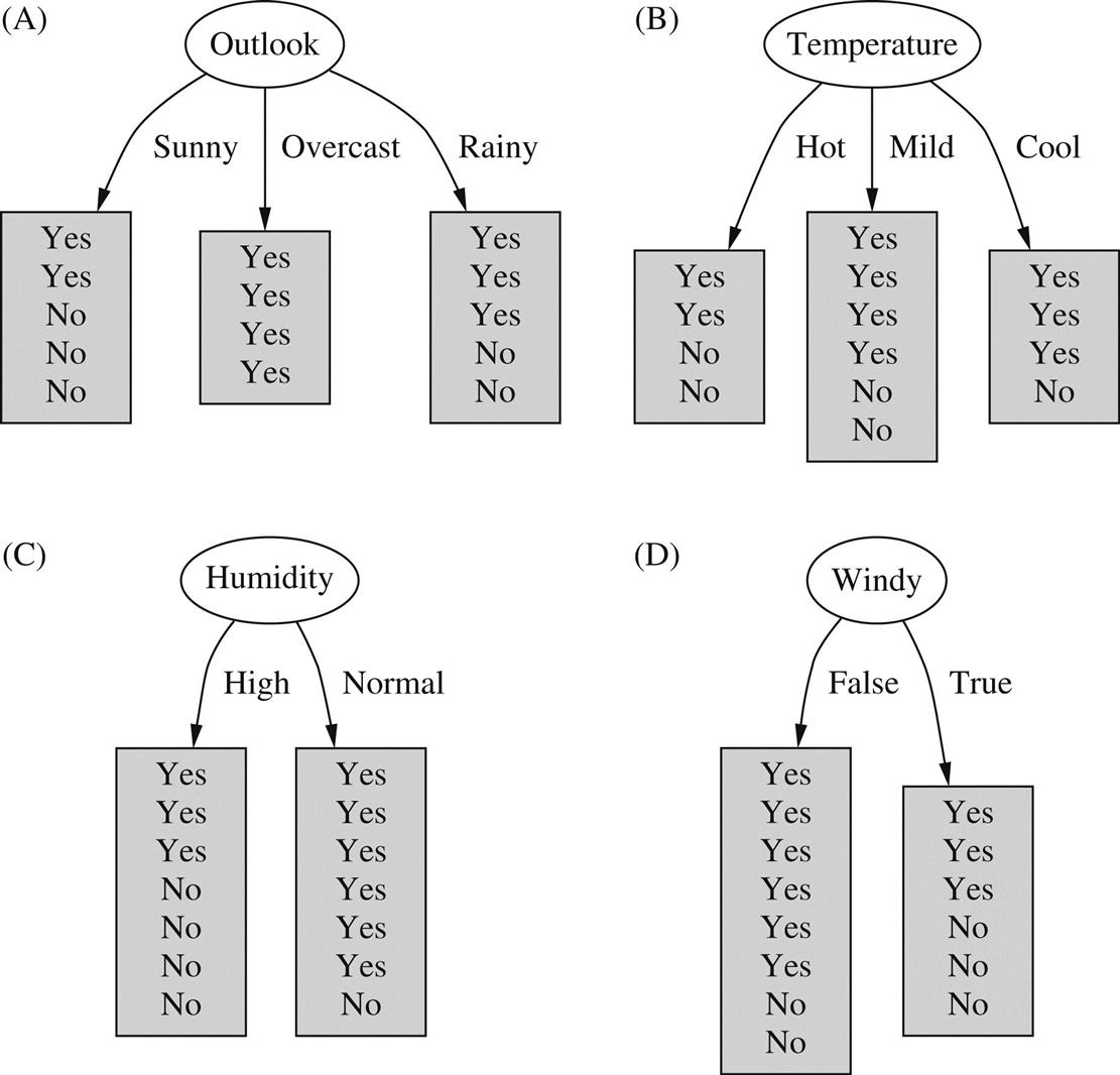
Figure 4.2 Tree stumps for the weather data.

The measure of purity that we will use is called the information and is measured in units called bits. Associated with a node of the tree, it represents the expected amount of information that would be needed to specify whether a new instance should be classified yes or no, given that the example reached that node. Unlike the bits in computer memory, the expected amount of information usually involves fractions of a bit—and is often less than one! It is calculated based on the number of yes and no classes at the node; we will look at the details of the calculation shortly. But first let’s see how it’s used. When evaluating the first tree in Fig. 4.2, the number of yes and no classes at the leaf nodes are [2, 3], [4, 0], and [3, 2], respectively, and the information values of these nodes are:

$\begin{array}{l} Info ([2, 3]) = 0.971 bits \\ Info ([4, 0]) = 0.0 bits \\ Info ([3, 2]) = 0.971 bits \end{array}$ $\begin{array}{l} Info ([2, 3]) = 0.971 bits \\ Info ([4, 0]) = 0.0 bits \\ Info ([3, 2]) = 0.971 bits \end{array}$

We calculate the average information value of these, taking into account the number of instances that go down each branch—five down the first and third and four down the second:

$\begin{array}{l} Info ([2, 3], [4, 0], [3, 2]) & = (5 / 14) \times 0.971 + (4 / 14) \times 0 + (5 / 14) \times 0.971 \\ = 0.693 bits . \end{array}$ $\begin{array}{l} Info ([2, 3], [4, 0], [3, 2]) & = (5 / 14) \times 0.971 + (4 / 14) \times 0 + (5 / 14) \times 0.971 \\ = 0.693 bits . \end{array}$

This average represents the amount of information that we expect would be necessary to specify the class of a new instance, given the tree structure in Fig. 4.2A.

Before any of the nascent tree structures in Fig. 4.2 were created, the training examples at the root comprised nine yes and five no nodes, corresponding to an information value of

$Info ([9, 5]) = 0.940 bits .$ $Info ([9, 5]) = 0.940 bits .$

Thus the tree in Fig. 4.2A is responsible for an information gain of

$\begin{array}{l} Gain (o u t l o o k) & = info ([9, 5]) - info ([2, 3], [4, 0], [3, 2]) = 0.940 - 0.693 \\ = 0.247 bits, \end{array}$ $\begin{array}{l} Gain (o u t l o o k) & = info ([9, 5]) - info ([2, 3], [4, 0], [3, 2]) = 0.940 - 0.693 \\ = 0.247 bits, \end{array}$

which can be interpreted as the informational value of creating a branch on the outlook attribute.

The way forward is clear. We calculate the information gain for each attribute and split on the one that gains the most information. In the situation of Fig. 4.2,

$\begin{array}{l} Gain (o u t l o o k) & = 0.247 bits \\ Gain (t e m p e r a t u r e) & = 0.029 bits \\ Gain (h u m i d i t y) & = 0.152 bits \\ Gain (w i n d y) & = 0.048 bits, \end{array}$ $\begin{array}{l} Gain (o u t l o o k) & = 0.247 bits \\ Gain (t e m p e r a t u r e) & = 0.029 bits \\ Gain (h u m i d i t y) & = 0.152 bits \\ Gain (w i n d y) & = 0.048 bits, \end{array}$

so we select outlook as the splitting attribute at the root of the tree. Hopefully this accords with your intuition as the best one to select. It is the only choice for which one daughter node is completely pure, and this gives it a considerable advantage over the other attributes. Humidity is the next best choice because it produces a larger daughter node that is almost completely pure.

Then we continue, recursively. Fig. 4.3 shows the possibilities for a further branch at the node reached when outlook is sunny. Clearly, a further split on outlook will produce nothing new, so we only consider the other three attributes. The information gain for each turns out to be

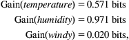
$\begin{array}{l} Gain (t e m p e r a t u r e) & = 0.571 bits \\ Gain (h u m i d i t y) & = 0.971 bits \\ Gain (w i n d y) & = 0.020 bits, \end{array}$ $\begin{array}{l} Gain (t e m p e r a t u r e) & = 0.571 bits \\ Gain (h u m i d i t y) & = 0.971 bits \\ Gain (w i n d y) & = 0.020 bits, \end{array}$

so we select humidity as the splitting attribute at this point. There is no need to split these nodes any further, so this branch is finished.

Figure 4.3 Expanded tree stumps for the weather data.

Continued application of the same idea leads to the decision tree of Fig. 4.4 for the weather data. Ideally the process terminates when all leaf nodes are pure, i.e., when they contain instances that all have the same classification. However, it might not be possible to reach this happy situation because there is nothing to stop the training set containing two examples with identical sets of attributes but different classes. Consequently we stop when the data cannot be split any further. Alternatively, one could stop if the information gain is zero. This is slightly more conservative, because it is possible to encounter cases where the data can be split into subsets exhibiting identical class distributions, which would make the information gain zero.

Figure 4.4 Decision tree for the weather data.

Calculating Information

Now it is time to explain how to calculate the information measure that is used as a basis for evaluating different splits. We describe the basic idea in this section, then in the next we examine a correction that is usually made to counter a bias toward selecting splits on attributes with large numbers of possible values.

Before examining the detailed formula for calculating the amount of information required to specify the class of an example given that it reaches a tree node with a certain number of yes’s and no’s, consider first the kind of properties we would expect this quantity to have:

1. When the number of either yes’s or no’s is zero, the information is zero;

2. When the number of yes’s and no’s is equal, the information reaches a maximum.

Moreover, the measure should be applicable to multiclass situations, not just to two-class ones.

The information measure relates to the amount of information obtained by making a decision, and a more subtle property of information can be derived by considering the nature of decisions. Decisions can be made in a single stage, or they can be made in several stages, and the amount of information involved is the same in both cases. For example, the decision involved in

$Info ([2, 3, 4])$ $Info ([2, 3, 4])$

can be made in two stages. First decide whether it’s the first case or one of the other two cases:

$Info ([2, 7])$ $Info ([2, 7])$

and then decide which of the other two cases it is:

$Info ([3, 4])$ $Info ([3, 4])$

In some cases the second decision will not need to be made, namely, when the decision turns out to be the first one. Taking this into account leads to the equation

$Info ([2, 3, 4]) = info ([2, 7]) + (7 / 9) \times info ([3, 4]) .$ $Info ([2, 3, 4]) = info ([2, 7]) + (7 / 9) \times info ([3, 4]) .$

Of course, there is nothing special about these particular numbers, and a similar relationship should hold regardless of the actual values. Thus we could add a further criterion to the list above:

3. The information should obey the multistage property that we have illustrated.

Remarkably, it turns out that there is only one function that satisfies all these properties, and it is known as the information value or entropy:

$Entropy (p_{1}, p_{2}, \dots, p_{n}) = - p_{1} \log p_{1} - p_{2} \log p_{2} \dots - p_{n} \log p_{n}$ $Entropy (p_{1}, p_{2}, \dots, p_{n}) = - p_{1} \log p_{1} - p_{2} \log p_{2} \dots - p_{n} \log p_{n}$

The reason for the minus signs is that logarithms of the fractions $p_{1}, p_{2}, .. ., p_{n}$ $p_{1}, p_{2}, .. ., p_{n}$ are negative, so the entropy is actually positive. Usually the logarithms are expressed in base 2, and then the entropy is in units called bits—just the usual kind of bits used with computers.

The arguments $p_{1}$ $p_{1}$ , $p_{2}$ $p_{2}$ ,… of the entropy formula are expressed as fractions that add up to one, so that, e.g.,

$Info ([2, 3, 4]) = entropy (2 / 9, 3 / 9, 4 / 9) .$ $Info ([2, 3, 4]) = entropy (2 / 9, 3 / 9, 4 / 9) .$

..................Content has been hidden....................

You can't read the all page of ebook, please click here login for view all page.

Table of Contents for Chapter 4. Algorithms: The basic methods

Create new playlist

Sign In

Sign Up

Algorithms

The basic methods

Abstracts

Keywords

4.1 Inferring Rudimentary Rules

Missing Values and Numeric Attributes

4.2 Simple Probabilistic Modeling

Missing Values and Numeric Attributes

Naïve Bayes for Document Classification

Remarks

4.3 Divide-and-Conquer: Constructing Decision Trees

Calculating Information

Table of Contents for
Chapter 4. Algorithms: The basic methods