
A popular forecasting tool is based on multiple linear regression models, using suitable predictors to capture trend and/or seasonality. In this chapter we show how a linear regression model can be set up to capture a time series with a trend and/or seasonality. The model, which is estimated from the training data, can then produce forecasts on future data by inserting the relevant predictor information into the estimated regression equation. We describe different types of common trends (linear, exponential, polynomial), as well as two types of seasonality (additive and multiplicative). Next, we show how a regression model can be used to quantify the correlation between neighboring values in a time series (called autocorrelation). This type of model, called an autoregressive model, is useful for improving forecast precision by making use of the information contained in the autocorrelation (beyond trend and seasonality). It is also useful for evaluating the predictability of a series (by evaluating whether the series is a "random walk"). The various steps of fitting linear regression and autoregressive models, using them to generate forecasts, and assessing their predictive accuracy, are illustrated using the Amtrak ridership series.
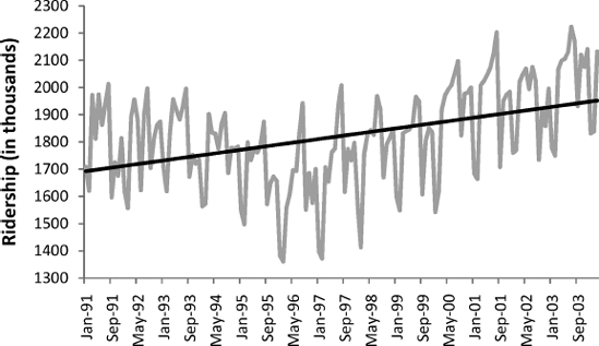
To create a linear regression model that captures a time series with a global linear trend, the output variable (Y) is set as the time series measurement or some function of it, and the predictor (X) is set as a time index. Let us consider a simple example, fitting a linear trend to the Amtrak ridership data. This type of trend is shown in Figure 16.1. From the time plot it is obvious that the global trend is not linear. However, we use this example to illustrate how a linear trend is fit, and later we consider more appropriate models for this series.
To obtain a linear relationship between Ridership and Time, we set the output variable Y as the Amtrak Ridership and create a new variable that is a time index t = 1,2,3,.... This time index is then used as a single predictor in the regression model:
where Yt is the Ridership at time point t and ɛ is the standard noise term in a linear regression. Thus, we are modeling three of the four time series components: level (β0), trend (β1), and noise (ɛ). Seasonality is not modeled. A snapshot of the two corresponding columns (Y and t) in Excel are shown in Figure 16.2.
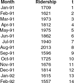
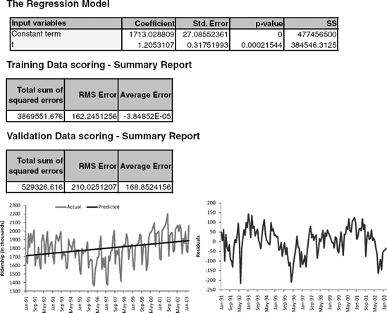
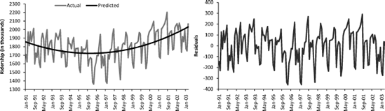
Figure 16.3. FITTED REGRESSION MODEL WITH LINEAR TREND. REGRESSION OUTPUT (TOP) AND TIME PLOTS OF ACTUAL AND FITTED SERIES (MIDDLE) AND RESIDUALS (BOTTOM)
After partitioning the data into training and validation sets, the next step is to fit a linear regression model to the training set, with t as the single predictor. Applying this to the Amtrak ridership data (with a validation set consisting of the last 12 months) results in the estimated model shown in Figure 16.3. The actual and fitted values and the residuals are shown in the two lower panels in time plots. Note that examining only the estimated coefficients and their statistical significance can be very misleading! In this example they would indicate that the linear fit is reasonable, although it is obvious from the time plots that the trend is not linear. The difference in the magnitude of the validation average error is also indicative of an inadequate trend shape. But an inadequate trend shape is easiest to detect by examining the series of residuals.
There are several alternative trend shapes that are useful and easy to fit via a linear regression model. Recall Excel's Trendline and other plots that help assess the type of trend in the data. One such shape is an exponential trend. An exponential trend implies a multiplicative increase/decrease of the series over time
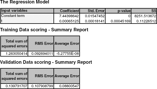
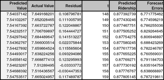
Note: As in the general case of linear regression, when comparing the predictive accuracy of models that have a different output variable, such as a linear model trend (with Y) and an exponential model trend (with log(Y)), it is essential to compare forecast or forecast errors on the same scale. An exponential trend model will produce forecasts of log(Y), and the forecast errors reported by the software will therefore be log(Y) – log(ŷ). To obtain forecasts in the original units, create a new column that takes an exponent of the model forecasts. Then, use this column to create an additional column of forecast errors, by subtracting the original Y. An example is shown in Figures 16.4 and Figure 16.5, where an exponential trend is fit to the Amtrak ridership data. Note that the performance measures for the training and validation data are not comparable to those from the linear trend model shown in Figure 16.3. Instead, we manually compute two new columns in Figure 16.5, one that gives forecasts of ridership (in thousands) and the other that gives the forecast errors in terms of ridership. To compare RMS Error or Average Error, we would now use the new forecast errors and compute their standard deviation (for RMS Error) or their average (for Average Error). These would then be comparable to the numbers in Figure 16.3.
Another nonlinear trend shape that is easy to fit via linear regression is a polynomial trend, and, in particular, a quadratic relationship of the form θ0 + θ1t + θ2t2 + ɛ. This is done by creating an additional predictor t2 (the square of t) and fitting a multiple linear regression with the two predictors t and t2 For the Amtrak ridership data, we have already seen a U-shaped trend in the data. We therefore fit a quadratic model, concluding from the plots of model fit and residuals (Figure 16.6) that this shape adequately captures the trend. The residuals now exhibit only seasonality.
In general, any type of trend shape can be fit as long as it has a mathematical representation. However, the underlying assumption is that this shape is applicable throughout the period of data that we have and also during the period that we are going to forecast. Do not choose an overly complex shape. Although it will fit the training data well, it will in fact be overfitting them. To avoid overfitting, always examine performance on the validation set and refrain from choosing overly complex trend patterns.
A seasonal pattern in a time series means that observations that fall in some seasons have consistently higher or lower values than those that fall in other seasons. Examples are day-of-week patterns, monthly patterns, and quarterly patterns. The Amtrak ridership monthly time series, as can be seen in the time plot, exhibits strong monthly seasonality (with highest traffic during summer months).
Seasonality is modeled in a regression model by creating a new categorical variable that denotes the season for each observation. This categorical variable is then turned into dummies, which in turn are included as predictors in the regression model. To illustrate this, we created a new Month column for the Amtrak ridership data, as shown in Figure 16.7.
In order to include the season categorical variable as a predictor in a regression model for Y (e.g., Ridership), we turn it into dummies. For m seasons we create m − 1 dummies, which are binary variables that take on the value 1 if the record falls in that particular season, and 0 otherwise.[40] We then partition the data into training and validation sets (see Section 15.5) and fit the regression model to the training data. The top panels of Figure 16.8 show the output of a linear regression fit to Ridership (Y) on 11-month dummies (using the training data). The fitted series and the residuals from this model are shown in the lower panels. The model appears to capture the seasonality in the data. However, since we have not included a trend component in the model (as shown in Section 16.1), the fitted values do not capture the existing trend. Therefore, the residuals, which are the difference between the actual and fitted values, clearly display the remaining U-shaped trend.
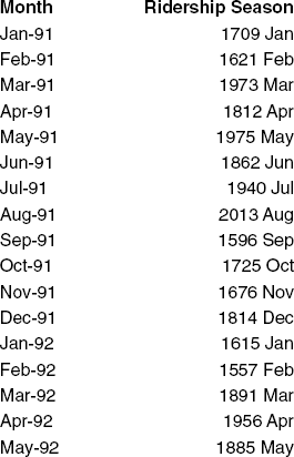
Figure 16.7. NEW CATEGORICAL VARIABLE (RIGHT) TO BE USED (VIA DUMMIES) AS PREDICTOR(S) IN A LINEAR REGRESSION MODEL
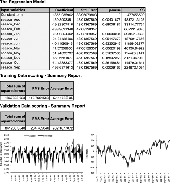
Figure 16.8. FITTED REGRESSION MODEL WITH SEASONALITY. REGRESSION OUTPUT (TOP), PLOTS OF FITTED AND ACTUAL SERIES (BOTTOM LEFT), AND MODEL RESIDUALS (BOTTOM RIGHT)
When seasonality is added as described above (create categorical seasonal variable, then create dummies from it, then regress on Y), it captures additive seasonality. This means that the average value of Y in a certain season is a certain amount more or less than that in another season. For example, in the Amtrak ridership, the coefficient for August (139.39) indicates that the average number of passengers in August is higher by 140,000 passengers than the average in April (the reference category). Using regression models, we can also capture multiplicative seasonality, where values on a certain season are on average higher or lower by a certain percentage compared to another season. To fit multiplicative seasonality, we use the same model as above, except that we use log(Y) as the output variable.
Finally, we can create models that capture both trend and seasonality by including predictors of both types. For example, from our exploration of the Amtrak Ridership data, it appears that a quadratic trend and monthly seasonality are both warranted. We therefore fit a model with 13 predictors: 11 dummies for month, and t and t2 for trend. The output and fit from this final model are shown in Figure 16.9. This model can then be used to generate k-step-ahead forecasts (denoted by Ft+k) by plugging in the appropriate month and index terms.
When we use linear regression for time series forecasting, we are able to account for patterns such as trend and seasonality. However, ordinary regression models do not account for dependence between observations, which in cross-sectional data is assumed to be absent. Yet, in the time series context, observations in neighboring periods tend to be correlated. Such correlation, called autocorrelation, is informative and can help in improving forecasts. If we know that a high value tends to be followed by high values (positive autocorrelation), then we can use that to adjust forecasts. We will now discuss how to compute the autocorrelation of a series and how best to utilize the information for improving forecasting.
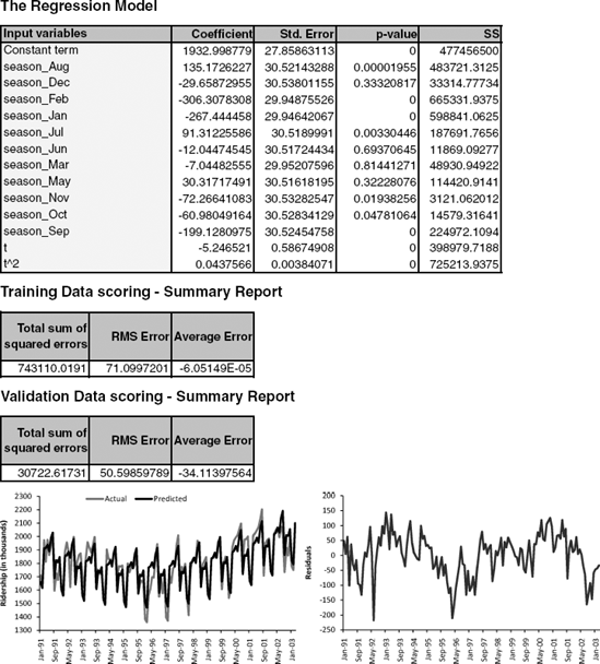
Figure 16.9. REGRESSION MODEL WITH MONTHLY (ADDITIVE) SEASONALITY AND QUADRATIC TREND, FIT TO AMTRAK RIDERSHIP DATA. REGRESSION OUTPUT (TOP), PLOTS OF FITTED AND ACTUAL SERIES (BOTTOM LEFT), AND MODEL RESIDUALS (BOTTOM RIGHT)
Correlation between values of a time series in neighboring periods is called autocorrelation because it describes a relationship between the series and itself. To compute autocorrelation, we compute the correlation between the series and a lagged version of the series. A lagged series is a "copy" of the original series, which is moved forward one or more time periods. A lagged series with lag 1 is the original series moved forward one time period; a lagged series with lag 2 is the original series moved forward two time periods, and so on. Table 16.1 shows the first 24 months of the Amtrak ridership series, the lag-1 series and the lag-2 series.
Table 16.1. FIRST 24 MONTHS OF AMTRAK RIDERSHIP SERIES
Month | Ridership | Lag-1 Series | Lag-2 Series |
|---|---|---|---|
Jan-91 | 1709 | ||
Feb-91 | 1621 | 1709 | |
Mar-91 | 1973 | 1621 | 1709 |
Apr-91 | 1812 | 1973 | 1621 |
May-91 | 1975 | 1812 | 1973 |
Jun-91 | 1862 | 1975 | 1812 |
Jul-91 | 1940 | 1862 | 1975 |
Aug-91 | 2013 | 1940 | 1862 |
Sep-91 | 1596 | 2013 | 1940 |
Oct-91 | 1725 | 1596 | 2013 |
Nov-91 | 1676 | 1725 | 1596 |
Dec-91 | 1814 | 1676 | 1725 |
Jan-92 | 1615 | 1814 | 1676 |
Feb-92 | 1557 | 1615 | 1814 |
Mar-92 | 1891 | 1557 | 1615 |
Apr-92 | 1956 | 1891 | 1557 |
May-92 | 1885 | 1956 | 1891 |
Jun-92 | 1623 | 1885 | 1956 |
Jul-92 | 1903 | 1623 | 1885 |
Aug-92 | 1997 | 1903 | 1623 |
Sep-92 | 1704 | 1997 | 1903 |
Oct-92 | 1810 | 1704 | 1997 |
Nov-92 | 1862 | 1810 | 1704 |
Dec-92 | 1875 | 1862 | 1810 |
Next, to compute the lag-1 autocorrelation (which measures the linear relationship between values in consecutive time periods), we compute the correlation between the original series and the lag-1 series (e.g., via the Excel function CORREL) to be 0.08. Note that although the original series shown in Table 16.1 has 24 time periods, the lag-1 autocorrelation will only be based on 23 pairs (because the lag-1 series does not have a value for Jan-91). Similarly, the lag-2 autocorrelation (measuring the relationship between values that are two time periods apart) is the correlation between the original series and the lag-2 series (yielding −0.15).
We can use XLMiner's ACF (autocorrelations) utility within the Time Series menu, to directly compute the autocorrelations of a series at different lags. For example, the output for the 24-month ridership is shown in Figure 16.10. To display a bar chart of the autocorrelations at different lags, check the Plot ACF option.
A few typical autocorrelation behaviors that are useful to explore are:
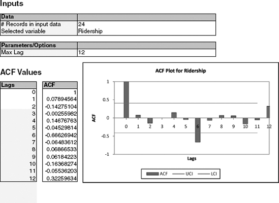
Figure 16.10. XLMINER OUTPUT SHOWING AUTOCORRELATION AT LAGS 1–12 FOR THE 24 MONTHS OF AMTRAK RIDERSHIP
Strong autocorrelation (positive or negative) at a lag larger than 1 typically reflects a cyclical pattern. For example, strong positive autocorrelation at lag 12 in monthly data will reflect an annual seasonality (where values during a given month each year are positively correlated).
Positive lag-1 autocorrelation (called "stickiness") describes a series where consecutive values move generally in the same direction. In the presence of a strong linear trend, we would expect to see a strong and positive lag-1 autocorrelation.
Negative lag-1 autocorrelation reflects swings in the series, where high values are immediately followed by low values and vice versa.
Examining the autocorrelation of a series can therefore help to detect seasonality patterns. In Figure 16.10, for example, we see that the strongest autocorrelation is at lag 6 and is negative. This indicates a biannual pattern in ridership, with 6-month switches from high to low ridership. A look at the time plot confirms the high-summer low-winter pattern.
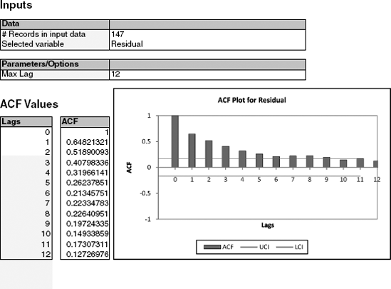
In addition to looking at autocorrelations of the raw series, it is very useful to look at autocorrelations of residual series. For example, after fitting a regression model (or using any other forecasting method), we can examine the autocorrelation of the series of residuals. If we have adequately modeled the seasonal pattern, then the residual series should show no autocorrelation at the season's lag. Figure 16.11 displays the autocorrelations for the residuals from the regression model with seasonality and quadratic trend shown in Figure 16.9. It is clear that the 6-month (and 12-month) cyclical behavior no longer dominates the series of residuals, indicating that the regression model captured them adequately. However, we can also see a strong positive autocorrelation from lag 1 on, indicating a positive relationship between neighboring residuals. This is valuable information, which can be used to improve forecasting.
In general, there are two approaches to taking advantage of autocorrelation. One is by directly building the autocorrelation into the regression model, and the other is by constructing a second-level forecasting model on the residual series.
Among regression-type models that directly account for autocorrelation are autoregressive models, or the more general class of models called ARIMA models (autoregressive integrated moving-average models). Autoregression models are similar to linear regression models, except that the predictors are the past values of the series. For example, an autoregression model of order 2 (AR(2)), can be written as
Estimating such models is roughly equivalent to fitting a linear regression model with the series as the output, and the lagged series (at lag 1 and 2 in this example) as the predictors. However, it is better to use designated ARIMA estimation methods (e.g., those available in XLMiner's Time Series> ARIMA menu) over ordinary linear regression estimation, to produce more accurate results. Moving from[41] AR to ARIMA models creates a larger set of more flexible forecasting models but also requires much more statistical expertise. Even with the simpler AR models, fitting them to raw time series that contain patterns such as trends and seasonality requires the user to perform several initial data transformations and to choose the order of the model. These are not straightforward tasks. Because ARIMA modeling is less robust and requires more experience and statistical expertise than other methods, the use of such models for forecasting raw series is generally less popular in practical forecasting. We therefore direct the interested reader to classic time series textbooks [e.g., see Chapter 4 in Chatfield (2003)].
However, we do discuss one particular use of AR models that is straightforward to apply in the context of forecasting, which can provide significant improvement to short-term forecasts. This relates to the second approach for utilizing autocorrelation, which requires constructing a second-level forecasting model for the residuals, as follows:
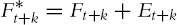
Generate k-step-ahead forecast of the series (Ft+k), using a forecasting method.
Generate k-step-ahead forecast of forecast error (Et+k), using an AR (or other) model.
Improve the initial k-step-ahead forecast of the series by adjusting it according to its forecasted error: Improved
In particular, we can fit low-order AR models to series of residuals (or forecast errors) that can then be used to forecast future forecast errors. By fitting the series of residuals, rather than the raw series, we avoid the need for initial data transformations (because the residual series is not expected to contain any trends or cyclical behavior besides autocorrelation).
To fit an AR model to the series of residuals, we first examine the autocorrelations of the residual series. We then choose the order of the AR model according to the lags in which autocorrelation appears. Often, when autocorrelation exists at lag 1 and higher, it is sufficient to fit an AR(1) model of the form
where Et denotes the residual (or forecast error) at time t. For example, although the autocorrelations in Figure 16.11 appear large from lags 1 to 10 or so, it is likely that an AR(1) would capture all these relationships. The reason is that if neighboring values are correlated, then the relationship can propagate to values that are two periods away, then three periods away, and so forth. The result of fitting an AR(1) model to the Amtrak ridership residual series is shown in Figure 16.12. The AR(1) coefficient (0.65) is close to the lag-1 autocorrelation that we found earlier (Figure 16.11). The forecasted residual for April 2003, given at the bottom, is computed by plugging in the most recent residual from March 2003 (equal to −33.786) into the AR(1) model: 0 + (0.647)(−33.786) = −21.866. The negative value tells us that the regression model will produce a ridership forecast for April 2003 that is too high and that we should adjust it down by subtracting 21,866 riders. In this particular example, the regression model (with quadratic trend and seasonality) produced a forecast of 2,115,000 riders, and the improved two-stage model [regression + AR(1) correction] corrected it by reducing it to 2,093,000 riders. The actual value for April 2003 turned out to be 2,099,000 riders—much closer to the improved forecast.
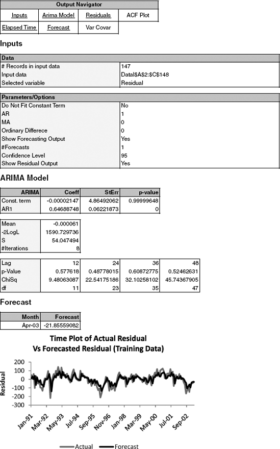
Finally, from the plot of the actual versus forecasted residual series, we can see that the AR(1) model fits the residual series quite well. Note, however, that the plot is based on the training data (until March 2003). To evaluate predictive performance of the two-level model [regression + AR(1)], we would have to examine performance (e.g., via MAPE or RMSE metrics) on the validation data, in a fashion similar to the calculation that we performed for April 2003 above.
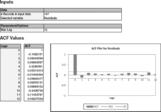
Finally, to examine whether we have indeed accounted for the autocorrelation in the series, and no more information remains in the series, we examine the autocorrelations of the series of residuals-of-residuals [the residuals obtained after the AR(1), which was applied to the regression residuals]. This can be seen in Figure 16.13. It is clear that no more autocorrelation remains, and that the addition of the AR(1) model has captured the autocorrelation information adequately.
We mentioned earlier that improving forecasts via an additional AR layer is useful for short-term forecasting. The reason is that an AR model of order k will usually only provide useful forecasts for the next k periods, and after that forecasts will rely on earlier forecasts rather than on actual data. For example, to forecast the residual of May 2003, when the time of prediction is March 2003, we would need the residual for April 2003. However, because that value is not available, it would be replaced by its forecast. Hence, the forecast for May 2003 would be based on the forecast for April 2003.
Before attempting to forecast a time series, it is important to determine whether it is predictable, in the sense that its past predicts its future. One useful way to assess predictability is to test whether the series is a random walk. A random walk is a series in which changes from one time period to the next are random. According to the efficient market hypothesis in economics, asset prices are random walks and therefore predicting stock prices is a game of chance.[42]
A random walk is a special case of an AR(1) model, where the slope coefficient is equal to 1:
We see from this equation that the difference between the values at periods t−1 and t is random, hence the term random walk. Forecasts from such a model are basically equal to the most recent observed value, reflecting the lack of any other information.
To test whether a series is a random walk, we fit an AR(1) model and test the hypothesis that the slope coefficient is equal to 1 (H0 : β1 = 1 vs H1 : β ≠ 1). If the hypothesis is accepted (reflected by a small p-value), then the series is not a random walk, and we can attempt to predict it.
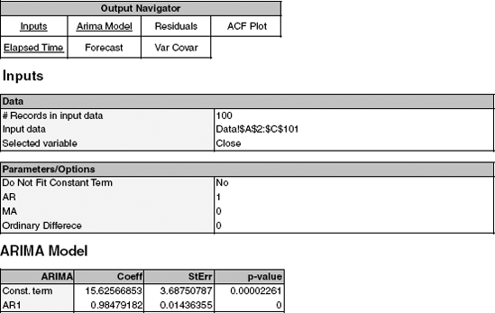
As an example, consider the AR(1) model shown in Figure 16.12. The slope coefficient (0.647) is more than 3 standard errors away from 1, indicating that this is not a random walk. In contrast, consider the AR(1) model fitted to the series of S&P500 monthly closing prices between May 1995 and August 2003 (available in SP500.xls, shown in Figure 16.14). Here the slope coefficient is 0.985, with a standard error of 0.015. The coefficient is sufficiently close to 1 (around one standard error away), indicating that this is a random walk. Forecasting this series using any of the methods described earlier is therefore futile.
16.1 Impact of September 11 on Air Travel in the United States: The Research and Innovative Technology Administration's Bureau of Transportation Statistics (BTS) conducted a study to evaluate the impact of the September 11, 2001, terrorist attack on U.S. transportation. The study report and the data can be found at
http://www.bts.gov/publications/estimatedimpacts of 9 11 on us travel. The goal of the study was stated as follows:The purpose of this study is to provide a greater understanding of the passenger travel behavior patterns of persons making long distance trips before and after 9/11.
The report analyzes monthly passenger movement data between January 1990 and May 2004. Data on three monthly time series are given in File Sept11Travel.xls for this period: (1) actual airline revenue passenger miles (Air), (2) rail passenger miles (Rail), and (3) vehicle miles traveled (Car).
In order to assess the impact of September 11, BTS took the following approach: using data before September 11, it forecasted future data (under the assumption of no terrorist attack). Then, BTS compared the forecasted series with the actual data to assess the impact of the event. Our first step, therefore, is to split each of the time series into two parts: pre-and post-September 11. We now concentrate only on the earlier time series.
Plot the pre-event Air time series.
Which time series components appear from the plot?
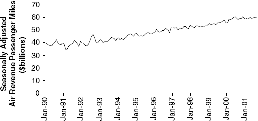
Figure 16.15 is a time plot of the seasonally adjusted pre-Sept-11 Air series. Which of the following methods would be adequate for forecasting this series?
Specify a linear regression model for the Air series that would produce a seasonally adjusted series similar to the one shown in (b), with multiplicative seasonality. What is the output variable? What are the predictors?
Run the regression model from (c). Remember to create dummy variables for the months (XLMiner will treat April as the reference category) and to use only pre-event data.
What can we learn from the statistical insignificance of the coefficients for October and September?
The actual value of Air (air revenue passenger miles) in January 1990 was 35.153577 billion. What is the residual for this month, using the regression model? Report the residual in terms of air revenue passenger miles.
Create an ACF (autocorrelation) plot of the regression residuals.
What does the ACF plot tell us about the regression model's forecasts?
How can this information be used to improve the model?
Fit linear regression models to Rail and to Auto, similar to the model you fit for Air. Remember to use only pre-event data. Once the models are estimated, use them to forecast each of the three postevent series.
For each series (Air, Rail, Auto), plot the complete pre-event and postevent actual series overlayed with the predicted series.
What can be said about the effect of the September 11 terrorist attack on the three modes of transportation? Discuss the magnitude of the effect, its time span, and any other relevant aspects.
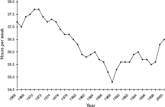
16.2 Analysis of Canadian Manufacturing Workers Workhours: The time series plot in Figure 16.16 describes the average annual number of weekly hours spent by Canadian manufacturing workers (data are available in CanadianWorkHours.xls, data courtesy of Ken Black).
Which one model of the following regression-based models would fit the series best?
Linear trend model
Linear trend model with seasonality
Quadratic trend model
Quadratic trend model with seasonality
If we computed the autocorrelation of this series, would the lag-1 autocorrelation exhibit negative, positive, or no autocorrelation? How can you see this from the plot?
Compute the autocorrelation and produce an ACF plot. Verify your answer to the previous question.
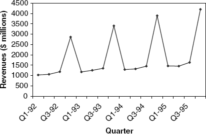
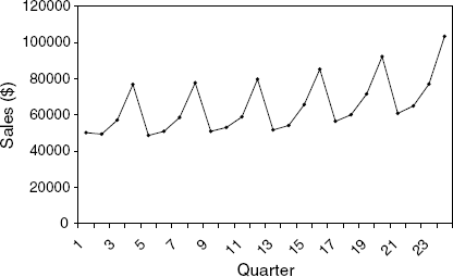
16.3 Regression Modeling of Toys "R" Us Revenues: Figure 16.17 is a time series plot of the quarterly revenues of Toys "R" Us between 1992 and 1995 (thanks to Chris Albright for suggesting the use of these data, which are available in ToysRUsRevenues.xls).
Fit a regression model with a linear trend and seasonal dummies. Use the entire series (excluding the last two quarters) as the training set.
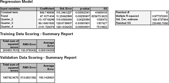
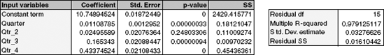
A partial output of the regression model is shown in Figure 16.18. Use this output to answer the following questions:
Mention two statistics (and their values) that measure how well this model fits the training data.
Mention two statistics (and their values) that measure the predictive accuracy of this model.
After adjusting for trend, what is the average difference between sales in Q3 and sales in Q1?
After adjusting for seasonality, which quarter (Q1, Q2, Q3 or Q4) has the highest average sales?
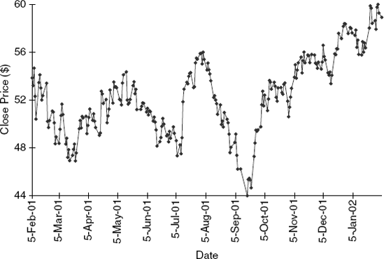
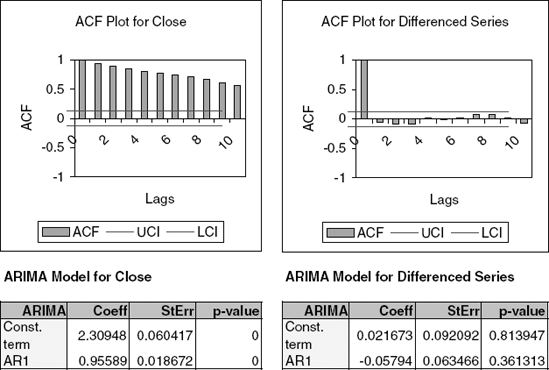
16.4 Forecasting Wal-Mart Stock: Figures 16.19 and Figures 16.20 show plots, summary statistics, and output from fitting an AR(1) model to the series of Wal-Mart daily closing prices between February 2001 and February 2002. (Thanks to Chris Albright for suggesting the use of these data, which are publicly available, e.g., at
http://finance.yahoo.comand are in the file WalMartStock.xls.) Use all the information to answer the following questions.Create a time plot of the differenced series.
Which of the following is/are relevant for testing whether this stock is a random walk?
Does the AR model indicate that this is a random walk? Explain how you reached your conclusion.
What are the implications of finding that a time series is a random walk? Choose the correct statement(s) below.
It is impossible to obtain useful forecasts of the series.
The series is random.
The changes in the series from one period to the other are random.
16.5 Forecasting Department Store Sales: The time series plot shown in Figure 16.21 describes actual quarterly sales for a department store over a 6-year period. (Data are available in DepartmentStoreSales.xls, data courtesy of Chris Albright.)
The forecaster decided that there is an exponential trend in the series. In order to fit a regression-based model that accounts for this trend, which of the following operations must be performed?
Take log of Quarter index
Take log of sales
Take an exponent of sales
Take an exponent of Quarter index
Fit a regression model with an exponential trend and seasonality, using only the first 20 quarters as the training data (remember to first partition the series into training and validation series).
A partial output is shown in Figure 16.22. From the output, after adjusting for trend, are Q2 average sales higher, lower, or approximately equal to the average Q1 sales?
Use this model to forecast sales in quarters 21 and 22.
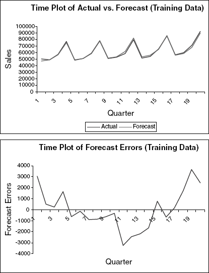
The plots in Figure 16.23 describe the fit (top) and forecast errors (bottom) from this regression model.
Recreate these plots.
Based on these plots, what can you say about your forecasts for quarters 21 and 22? Are they likely to overforecast, underforecast, or be reasonably close to the real sales values?
Looking at the residual plot, which of the following statements appear true?
Seasonality is not captured well.
The regression model fits the data well.
The trend in the data is not captured well by the model.
Which of the following solutions is adequate and a parsimonious solution for improving model fit?
Fit a quadratic trend model to the residuals (with Quarter and Quarter2.)
Fit an AR model to the residuals.
Fit a quadratic trend model to Sales (with Quarter and Quarter2.)
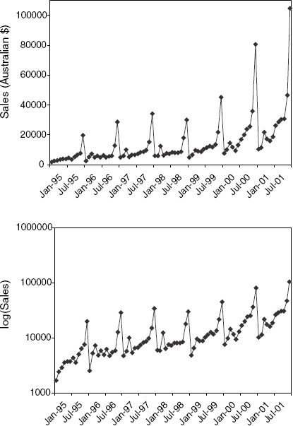
16.6 Souvenir Sales:Figure 16.24 shows a time plot of monthly sales for a souvenir shop at a beach resort town in Queensland, Australia, between 1995 and 2001. [Data are available in SouvenirSales.xls, source: R. J. Hyndman, Time Series Data Library,
http://www.robjhyndman.com/TSDL; accessed on December 28, 2009.] The series is presented twice, in Australian dollars and in log scale. Back in 2001, the store wanted to use the data to forecast sales for the next 12 months (year 2002). It hired an analyst to generate forecasts. The analyst first partitioned the data into training and validation sets, with the validation set containing the last 12 months of data (year 2001). She then fit a regression model to sales, using the training set.Based on the two time plots, which predictors should be included in the regression model? What is the total number of predictors in the model?
Run a regression model with Sales (in Australian dollars) as the output variable and with a linear trend and monthly predictors. Remember to fit only the training data. Call this model A.
Examine the estimated coefficients: Which model tends to have the highest average sales during the year? Why is this reasonable?
The estimated trend coefficient is 245.36. What does this mean?
Run a regression model with log(Sales) as the output variable and with a linear trend and monthly predictors. Remember to fit only the training data. Call this model B.
Fitting a model to log(Sales) with a linear trend is equivalent to fitting a model to Sales (in dollars) with what type of trend?
The estimated trend coefficient is 0.2. What does this mean?
Use this model to forecast the sales in February 2002. What is the extra step needed?
Compare the two regression models (A and B) in terms of forecast performance. Which model is preferable for forecasting? Mention at least two reasons based on the information in the outputs.
Continuing with model B [with log(Sales) as output], create an ACF plot until lag 15. Now fit an AR model with lag 2 [ARIMA(2,0,0)].
Examining the ACF plot and the estimated coefficients of the AR(2) model (and their statistical significance), what can we learn about the forecasts that result from model B?
Use the autocorrelation information to compute an improved forecast for January 2002, using model B and the AR(2) model above.
How would you model these data differently if the goal was to understand the different components of sales in the souvenir shop between 1995 and 2001? Mention two differences.
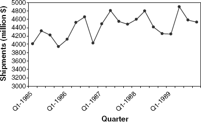
16.7 Shipments of Household Appliances: The time plot in Figure 16.25 shows the series of quarterly shipments (in million dollars) of U.S. household appliances between 1985 and 1989. (Data are available in ApplianceShipments.xls; data courtesy of Ken Black.)
If we compute the autocorrelation of the series, which lag (>0) is most likely to have the largest coefficient (in absolute value)? Create an ACF plot and compare with your answer.
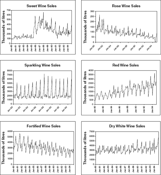
16.8 Forecasting Australian Wine Sales:Figure 16.26 shows time plots of monthly sales of six types of Australian wines (red, rose, sweet white, dry white, sparkling, and fortified) for 1980–1994. [Data are available in AustralianWines.xls, source: R. J. Hyndman, Time Series Data Library,
http://www.robjhyndman.com/TSDL; accessed on December 28, 2009.] The units are thousands of liters. You are hired to obtain short-term forecasts (2–3 months ahead) for each of the six series, and this task will be repeated every month.Which forecasting method would you choose if you had to choose the same method for all series except Sweet Wine? Why?
Fortified wine has the largest market share of the six types of wine considered. You are asked to focus on fortified wine sales alone and produce as accurate as possible forecast for the next 2 months.
Start by partitioning the data using the period until December 1993 as the training set.
Fit a regression model to sales with a linear trend and seasonality.
Comparing the "actual vs. forecast" plots for the two models, what does the similarity between the plots tell us?
Use the regression model to forecast sales in January and February 1994.
Create an ACF plot for the residuals from the above model until lag 12.
Examining this plot, which of the following statements are reasonable?
Decembers (month 12) are not captured well by the model.
There is a strong correlation between sales on the same calendar month.
The model does not capture the seasonality well.
We should try to fit an autoregressive model with lag 12 to the residuals.
[39] Data Mining for Business Intelligence, By Galit Shmueli, Nitin R. Patel, and Peter C. Bruce Copyright © 2010 Statistics.com and Galit Shmueli
[40] We use only m − 1 dummies because information about the m − 1 seasons is sufficient. If all m variables are zero, then the season must be the mth season. Including the mth variable would ca redundant information and multicollinearity errors.
[41] ARIMA model estimation differs from ordinary regression estimation by accounting for the dependence between observations.
[42] There is some controversy surrounding the efficient market hypothesis, with claims that there is slight autocorrelation in asset prices, which does make them predictable to some extent. However, transaction costs and bid-ask spreads tend to offset any prediction benefits.