
Chapter
3
Storage Arrays
TOPICS COVERED IN THIS CHAPTER:
- Enterprise-class and midrange storage arrays
- Block storage arrays and NAS storage arrays
- Flash-based storage arrays
- Storage array architectures
- Array-based replication and snapshot technologies
- Thin provisioning
- Space efficiency
- Auto-tiering
- Storage virtualization
- Host-integration technologies
 This chapter builds on the previous foundational knowledge covered in Chapter 2, “Storage Devices,” and shows how various drive technologies are pooled together and utilized in storage arrays. It covers the major types of storage arrays used by most businesses worldwide, including Storage Area Network (SAN) and Network Attached Storage (NAS) arrays. You will learn how they integrate with host operating systems, hypervisors, and applications, as well as about the advanced features commonly found in storage arrays. These features include technologies that play a significant role in business continuity planning, such as remote replication and local snapshots. They also include space-efficiency technologies that help improve storage utilization and bring down the cost of running a storage environment—technologies such as thin provisioning, auto-tiering, deduplication, and compression.
Storage Arrays—Setting the Scene
Q. Holy cow! What's that huge old piece of tin in the corner of the data center?
A. That's the storage array!
Traditionally, storage arrays have been big, honking frames of spinning disks that took up massive amounts of data-center floor space and sucked enough electricity to power a small country. The largest could be over 10 cabinets long, housing thousands of disk drives, hundreds of front-end ports, and terabytes of cache. They tended to come in specialized cabinets that were a data-center manager's worst nightmare. On top of that, they were expensive to buy, complicated to manage, and about as inflexible as granite. That was excellent if you wanted to make a lot of money as a consultant, but not so good if you wanted to run a lean and efficient IT shop that could respond quickly to business demands.
Figure 3.1 shows an 11-frame EMC VMAX array.
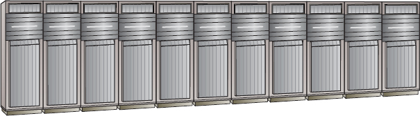
Thankfully, this is all changing, in no small part because of the influence of solid-state storage and the cloud. Both technologies are hugely disruptive and are forcing storage vendors to up their game. Storage arrays are becoming more energy efficient, simpler to manage, more application and hypervisor aware, smaller, more standardized, and in some cases cheaper!
Here is a quick bit of terminology before you get into the details: the terms storage array, storage subsystem, storage frame, and SAN array are often used to refer to the same thing. While it might not be the most technically accurate, this book predominantly uses the term storage array or just array, as they're probably the most widely used terms in the industry.

You will sometimes hear people referring to a storage array as a SAN. This is outright wrong. A SAN is a dedicated storage network used for connecting storage arrays and hosts.
On to the details.
What Is a Storage Array?
A storage array is a computer system designed for and dedicated to providing storage to externally attached computers, usually via a storage network. This storage has traditionally been spinning disk, but we are seeing an increasing number of solid-state media in storage arrays. It is not uncommon for a large storage array to have more than a petabyte (PB) of storage.
Storage arrays connect to host computers over a shared network and typically provide advanced reliability and enhanced functionality. Storage arrays come in three major flavors:
- SAN
- NAS
- Unified (SAN and NAS)
SAN storage arrays, sometimes referred to as block storage arrays, provide connectivity via block-based protocols such as Fibre Channel (FC), Fibre Channel over Ethernet (FCoE), Internet Small Computer System Interface (iSCSI), or Serial Attached SCSI (SAS). Block storage arrays send low-level disk-drive access commands called SCSI command descriptor blocks (CDBs) such as READ block, WRITE block, and READ CAPACITY over the SAN.
NAS storage arrays, sometimes called filers, provide connectivity over file-based protocols such as Network File System (NFS) and SMB/CIFS. File-based protocols work at a higher level than low-level block commands. They manipulate files and directories with commands that do things such as create files, rename files, lock a byte range within a file, close a file, and so on.
Although the protocol is actually Server Message Block (SMB), more often than not it is referred to by its legacy name, Common Internet File System (CIFS). It is pronounced sifs.
Unified storage arrays, sometimes referred to as multiprotocol arrays, provide shared storage over both block and file protocols. The best of both worlds, right? Sometimes, and sometimes not.
The purpose of all storage arrays, SAN and NAS, is to pool together storage resources and make those resources available to hosts connected over the storage network. Over and above this, most storage arrays provide the following advanced features and functionality:
- Replication
- Snapshots
- Offloads
- High availability and resiliency
- High performance
- Space efficiency
While there are all kinds of storage arrays, it is a nonfunctional goal of every storage array to provide the ultimate environment and ecosystem for disk drives and solid-state drives to survive and thrive. These arrays are designed and finely tuned to provide an optimally cooling airflow, vibration dampening, and a clean protected power supply, as well as performing tasks such as regular scrubbing of disks and other health checking. Basically, if you were a disk drive, you would want to live in a storage array!
SCSI Enclosure Services (SES) is one example of the kinds of services storage arrays provide for disk drives. SES is a background technology that you may never need to know about, but it provides a vital service. SES monitors power and voltages, fans and cooling, midplanes, and other environmentally related factors in your storage array. In lights-out data centers, SES can alert you to the fact that you may have a family of pigeons nesting in the warm backend of your tier 1 production storage array.
SAN Storage
As noted earlier, SAN storage arrays provide connectivity to storage resources via block-based protocols such as FC, FCoE, and iSCSI. Storage resources are presented to hosts as SCSI logical unit numbers (LUNs). Think of a LUN as a raw disk device that, as far as the operating system or hypervisor is concerned, looks and behaves exactly like a locally installed disk drive—basically, a chunk of raw capacity. As such, the OS/hypervisor knows that it needs to format the LUN and write a filesystem to it.
While somewhat debatable, when compared to NAS storage, SAN storage arrays have historically been perceived as higher performance and higher cost. They provide all the snapshot and replication services that you would also get on a NAS array, but as SAN storage arrays do not own or have any knowledge of the filesystem on a volume, in some respects they are a little dumb compared to their NAS cousins.
One of the major reasons that SAN arrays have been viewed as higher performance than NAS arrays is because of the dedicated Fibre Channel network that is often required for a SAN array. Fibre Channel networks are usually dedicated to storage traffic, often employing cut-through switching techniques, and operate at high-throughput levels. Therefore, they usually operate at a significantly lower latency than sharing a 1 Gigabit or even 10 Gigabit Ethernet network, which are common when using a NAS array.
NAS Storage
NAS storage arrays work with files rather than blocks. These arrays provide connectivity via TCP/IP-based file-sharing protocols such as NFS and SMB/CIFS. They are often used to consolidate Windows and Linux file servers, where hosts mount exports and shares from the NAS in exactly the same way they would mount an NFS or CIFS share from a Linux or Windows file server. Because of this, hosts know that these exports and shares are not local volumes, meaning there is no need to write a filesystem to the mounted volume, as this is the job of the NAS array.
A Windows host wanting to map an SMB/CIFS share from a NAS array will do so in exactly the same way as it would map a share from a Windows file server by using a Universal Naming Convention (UNC) path such as \legendary-file-servershares ech.
Because NAS protocols operate over shared Ethernet networks, they usually suffer from higher network-based latency than SAN storage and are more prone to network-related issues. Also, because NAS storage arrays work with files and directories, they have to deal with file permissions, user accounts, Active Directory, Network Information Service (NIS), file locking, and other file-related technologies. One common challenge is integrating virus checking with NAS storage. There is no doubt about it: NAS storage is an entirely different beast than SAN storage.
NAS arrays are often referred to using the NetApp term filers, so it would not be uncommon to hear somebody say, “We're upgrading the code on the production filers this weekend.” NAS controllers are often referred to as heads or NAS heads. So a statement such as, “The vendor is on site replacing a failed head on the New York NAS” refers to replacing a failed NAS controller.
NAS arrays have historically been viewed as cheaper and lower performance than SAN arrays. This is not necessarily the case. In fact, because NAS arrays own and understand the underlying filesystem in use on an exported volume, and therefore understand files and metadata, they can often have the upper hand over SAN arrays. As with most things, you can buy cheap, low-performance NAS devices, or you can dig a little deeper and buy expensive, high-performance NAS. Of course, most vendors will tell you that their NAS devices are low cost and high performance. Just be sure you know what you are buying before you part with your company's hard-earned cash.
Unified Storage
Unified arrays provide block- and file-based storage—SAN and NAS. Different vendors implement unified arrays in different ways, but the net result is a network storage array that allows storage resources to be accessed by hosts either as block LUNs over block protocols or as network shares over file-sharing protocols. These arrays work well for customers with applications that require block-based storage, such as Microsoft Exchange Server, but may also want to consolidate file servers and use a NAS array.
Sometimes these so-called unified arrays are literally a SAN array and a NAS array, each with its own dedicated disks, bolted together with a shiny door slapped on the front to hide the hodgepodge behind. Arrays like this are affectionately referred to as Frankenstorage. The alternative to the Frankenstorage design is to have a single array with a common pool of drives running a single microcode program that handles both block and file.
There are arguments for and against each design approach. The Frankenstorage design tends to be more wasteful of resources and harder to manage, but it can provide better and more predictable performance, as the SAN and NAS components are actually air-gapped and running as isolated systems if you look under the hood. Generally speaking, bolting a SAN array and a NAS array together with only a common GUI is not a great design and indicates legacy technology.
Storage Array Architecture Whistle-Stop Tour
In this section, you'll examine the major components common to most storage array architectures in order to set the foundation for the rest of this chapter.
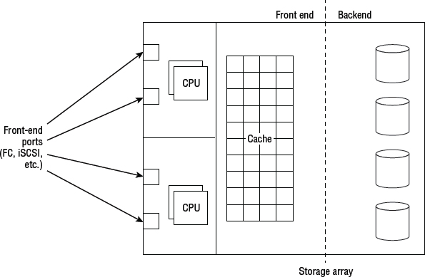
Figure 3.2 shows a high-level block diagram of a storage array—SAN or NAS—outlining the major components.
Starting from the left, we have front-end ports. These connect to the storage network and allow hosts to access and use exported storage resources. Front-end ports are usually FC or Ethernet (iSCSI, FCoE, NFS, SMB). Hosts that wish to use shared resources from the storage array must connect to the network via the same protocol as the storage array. So if you want to access block LUNs over Fibre Channel, you need a Fibre Channel host bus adapter (HBA) installed in your server.
If we move to the right of the front-end ports, we hit the processors. These are now almost always Intel CPUs. They run the array firmware and control the front-end ports and the I/O that comes in and out over them.
If we keep moving right, behind the processors is cache memory. This is used to accelerate array performance, and in mechanical disk-based arrays is absolutely critical to decent performance. No cache, no performance!
Once leaving cache, you are into the realm of the backend. Here there could be more CPUs, and ports that connect to the drives that compose the major part of the backend. Sometimes the same CPUs that control the front end also control the backend.
Storage array architecture is discussed in greater detail in the “The Anatomy of a Storage Array” section later in this chapter.
Architectural Principles
Now let's look at some of the major architectural principles common to storage arrays.
Redundancy
Redundancy in IT designs is the principle of having more than one of every component so that when (not if) you experience component failures, your systems are able to stay up and continue providing service. Redundant designs are often N+1, meaning that each component (N) has one spare component that can take on the load if N fails. Redundant IT design is the bedrock for always-on enterprises in the digital age, where even small amounts of downtime can be disastrous for businesses.
Different storage arrays are built with different levels of redundancy—and you get what you pay for. Cheap arrays will come with minimal redundant parts, whereas enterprise-class arrays will come with redundancy built in to nearly every component—power supplies, front-end ports, CPUs, internal pathways, cache modules, drive shelves, and drives. Most of these components are hot-swappable. The end goal is for the array to be able to roll with the punches and continue servicing I/O despite suffering multiple component failures.
Hot swap refers to the ability to replace physical components within a computer system without needing to power it down. A common example is the disk drive, which should always be capable of being replaced while the system is up and servicing I/O.
![]() Real World Scenario
Real World Scenario
An Example of Major Maintenance Performed with System Still Online
A company spent a long time troubleshooting an intermittent issue on the backend of one of their storage arrays. The issue was not major but was enough to warrant investigation. The vendor struggled to pin down the root cause of the issue and carried out a systematic plan of replacing multiple components that could be the root cause. They started by replacing the simplest components and worked their way through all possible components until only one component was left. The components they replaced included the following: disk drives, disk-drive magazines, fiber cables, backend ports, and Fibre Channel Arbitrated Loop (FC-AL) modules. All of these components were redundant and were replaced while the system was online. No connected hosts were aware of the maintenance, and no service impact was experienced. After replacing all these components, the fault persisted, and the midplane in a drive enclosure had to be swapped out. As this procedure required powering down an entire drive enclosure, removing all the drives, swapping out the midplane, and putting it all back together again, it was considered high risk and was carried out over a weekend. Although an entire drive enclosure was powered down, was removed, had components replaced, and then was powered back up, no service interruption was experienced. The system as a whole stayed up, and as far as connected systems were concerned, nothing was going on. It was all transparent to connected hosts and applications.
Dual-Controller Architectures
Dual-controller architectures are exactly what they sound like: storage arrays with two controllers.
Controllers are often referred to by other names such as nodes or engines, and commonly as heads in the NAS world.
In almost all dual-controller configurations, while both controllers are active at the same time, they are not truly active/active. Each LUN is owned by only one of the controllers. It is common for odd-numbered LUNs to be owned by one controller, while even-numbered LUNs are owned by the other controller. Only the controller that owns the LUN can read and write directly to it. In this sense, dual-controller arrays are active/passive on a per LUN basis—one controller owns the LUN and is therefore active for that LUN, whereas the other controller is passive and does not read and write directly to it. This is known as asymmetric logical unit access (ALUA).
If a host accesses a LUN via the non-owning controller, the non-owning controller will have to forward the request to the owning controller, adding latency to the process. If this situation persists, the ownership of the LUN (the controller that owns and can read and write directly to the LUN) should be changed. Special software installed on the host, referred to as multipathing software, helps manage this, and controller ownership is usually automatically changed by the system without user intervention.
Let's look at a quick example of a dual-controller system implementing ALUA. Say you have a dual-controller system with one controller called CTL0 and the other named CTL1. This system has 10 LUNs. CTL0 owns all the odd-numbered LUNs, and CTL1 owns all the even-numbered LUNs. When I say a controller owns a LUN, I mean it has exclusive read-and-write capability to that LUN. In this configuration, you can see that both controllers are active—hence the reason some people refer to them as active/active. However, only a single controller has read/write access to any LUN at any point in time.
Here is the small print: should one of the controllers fail in a dual-controller system, the surviving controller seizes ownership of the LUNs that were previously owned by the failed controller. Great—this might seem fine, until you realize that you have probably doubled the workload of the surviving controller. And if both controllers were already busy, the surviving controller could end up with more work than it can handle. This is never a good place to be! The moral of the story is to plan for failures and don't overload your systems.
Dual-controller systems have been around for years and are relatively simple to implement and cheap to purchase. As a result. they are popular in small- to medium-sized environments and are often referred to as midrange arrays.
Dual-Controller Shortcomings
The following are the major gotchas you should be aware of with dual-controller architectures:
- When one controller fails, the other controller assumes the workload of the failed controller. Obviously, this increases the workload of the surviving controller. It should be easy to see that a dual-controller array with both controllers operating at 80 percent of designed capacity will have performance issues if one controller fails.
- When a controller fails in a dual-controller system, the system has to go into what is known as write-through mode. In this mode, I/O has to be secured to the backend disk before an acknowledgment (ACK) is issued to the host. This is important, because issuing an ACK when the data is in cache (but not mirrored to the other controller because it is down) would result in data being lost if the surviving controller also failed. Because write-through mode does not issue an ACK when I/O hits cache, performance is severely impacted!
- Dual-controller architectures are severely limited in scalability and cannot have more than two controller nodes.
I've seen many performance issues arise in production environments that push dual-controller arrays to their limit, only to have the surviving controller unable to cope with the load when one of the controllers fails. On more than one occasion, I have seen email systems unable to send and receive mail in a timely manner when the underlying storage array is forced to run on a single controller. Even when the failed controller is replaced, the mail queues can take hours, sometimes days, to process the backlog and return to normal service. It is not good to be the email or storage admin/architect when this kind of thing happens!
Grid Storage Architectures
Grid storage architectures, sometimes referred to as clustered or scale-out architectures, are the answer to the limitations of dual-controller architectures. They consist of more than two controllers and are far more modern and better suited to today's requirements than legacy dual-controller architectures.
True Active/Active LUN Ownership
The major design difference when compared to the majority of dual-controller architectures is that all controllers in a grid-based array act as a single logical unit and therefore operate in a true active/active configuration. When saying true active/active, I mean that it's not limited to any of the ALUA shenanigans that we are restricted to with dual-controller architectures. In grid architectures, multiple nodes can own and write to any and all LUNs. This means that a host can issue I/O to a LUN over any of the available paths to the LUN it has, without adding the latency that occurs when a non-owning controller has to forward the request to the owning controller. In contrast, with dual-controller arrays, the host can issue I/O to a particular LUN only over paths to the owning controller without incurring additional latency.
The term scale-out means that you can independently add more nodes, which can contain CPUs, memory, and ports to the system, as well as more drives. This is different from scale-up systems, which can add only more drives.
Let's revisit our simple example from the “Dual-Controller Architectures” section, where we have 10 LUNs on our array, this time in a four-controller array. As this is a grid architecture, all four nodes can be active for, and write to, all 10 LUNs. This can significantly improve performance.
Seamless Controller Failures
Grid storage arrays can also deal more gracefully with controller failures. This is because they should not have to go into cache write-through mode—I say should not, because not all arrays are clever enough to do this. A four-node array with a single failed controller will still have three controllers up and working. There is no reason, other than poor design, that these surviving three controllers should not be able to continue providing a mirrored (protected) cache, albeit smaller in usable capacity, while the failed controller is replaced.
Here is a quick example: Assume each controller in our four-controller array has 10 GB of cache, for a system total of 40 GB of cache. For simplicity's sake, let's assume the cache is protected by mirroring, meaning half of the 40 GB is usable—20 GB. When a single controller fails, the total cache available will be reduced to 30 GB. This can still be mirror protected across the surviving three controllers, leaving ~15 GB of usable cache. The important point is that although the amount of cache is reduced, the system does not have to go into cache write-through mode. This results in a significantly reduced performance hit during node failures.
Also, a four-node array that loses a single controller node has its performance (CPUs, cache, and front-end port count) reduced by only 25 percent rather than 50 percent. Likewise, an eight-node array will have performance reduced by only 12.5 percent. Add this on top of not having to go into cache write-through mode, and you have a far more reliable and fault-tolerant system.
Scale-Out Capability
Grid arrays also scale far better than dual-controller arrays. This is because you can add CPU, cache, bandwidth, and disks. Dual-controller architectures often allow you to add only drives.
Assume that you have a controller that can deal with 10,000 Input/Output Operations Per Second (IOPS). A dual-controller array based on these controllers can handle a maximum of 20,000 IOPS—although if one of the controllers fails, this number will drop back down to 10,000. Even if you add enough disk drives behind the controllers to be able to handle 40,000 IOPS, the controllers on the front end will never be able to push the drives to their 40,000 IOPS potential. If this were a grid-based architecture, you could also add more controllers to the front end, so that the front end would be powerful enough to push the drives to their limit.
This increased scalability, performance, and resiliency comes at a cost! Grid-based arrays are usually considered enterprise class and sport an appropriately higher price tag.
Enterprise-Class Arrays
You will often hear people refer to arrays as being enterprise class. What does this mean? Sadly, there is no official definition, and vendors are prone to abusing the term. But typically, the term enterprise class suggests the following:
- Multiple controllers
- Minimal impact when controllers fail
- Online nondisruptive upgrades (NDUs)
- Scale to over 1,000 drives
- High availability
- High performance
- Scalable
- Always on
- Predictable performance
- Expensive!
The list could go on, but basically enterprise class is what you would buy every time if you could afford to!
Most storage vendors will offer both midrange and enterprise-class arrays. Generally speaking, grid-based architectures fall into the enterprise-class category, whereas dual-controller architectures are often considered midrange.
Indestructible Enterprise-Class Arrays
Enterprise-class arrays are the top dog in the storage array world, and it's not uncommon for vendors to use superlatives such as bulletproof or indestructible to describe their enterprise-class babies.
On one occasion, HP went to the extent of setting up one of their enterprise-class XP arrays in a lab and firing a bullet through it to prove that it was bulletproof. The bullet passed all the way through the array without causing an issue. Of course, the bullet took out only half of the array's controller logic, and the workload was specifically designed so as not to be affected by destroyed components. But nonetheless, it was a decent piece of marketing.
On another occasion, HP configured two of their XP enterprise-class arrays in a replicated configuration and blew up one of the arrays with explosives. The surviving array picked up the workload and continued to service the connected application.
Both are a tad extreme but good fun to watch on YouTube.
Some people argue that for an array to be truly enterprise class, it must support mainframe attachment. True, all mainframe-supporting arrays are enterprise class, but not all enterprise-class arrays support mainframe!
Midrange Arrays
Whereas enterprise arrays have all the bells and whistles and are aimed at customers with deep pockets, midrange arrays are targeted more toward the cost-conscious customer. Consequently, midrange arrays are more commonly associated with dual-controller architectures.
While midrange arrays are by no means bad, they definitely lag behind enterprise arrays in the following areas:
- Performance
- Scalability
- Availability
However, they tend to come in at significantly lower costs (for both capital expenditures and operating expenditures).
Referring to an array as midrange indicates that it is not quite low-end. Although these arrays might not be in the same league as enterprise arrays, they often come with good performance, availability, and a decent feature-set for a more palatable price.
All-Flash Arrays
As far as storage and IT administrators are concerned, all-flash storage arrays operate and behave much the same as traditional storage arrays, only faster! Or at least that is the aim. By saying that they behave the same, I mean that they have front-end ports, usually some DRAM cache, internal buses, backend drives, and the like. They take flash drives, pool them together, carve them into volumes, and protect them via RAID or some other similar protection scheme. Many even offer snapshot and replication services, thin provisioning, deduplication, and compression. All-flash arrays can be dual-controller, single-controller, or scale-out (and no doubt anything else that appears in the future).
However, there are subtle and significant differences under the hood that you need to be aware of. Let's take a look.
Solid-state technology is shaking up the storage industry and changing most of the rules! This means that you cannot simply take a legacy architecture that has been designed and fine-tuned over the years to play well with spinning disk, and lash it full of solid-state technology. Actually, you can do this, and some vendors have, but you will absolutely not be getting the most from your array or the solid-state technology you put in it.
Solid-state storage changes most of the rules because it behaves so differently than spinning disk. This means that all the fine-tuning that has gone into storage array design over the last 20+ years—massive front-end caches, optimized data placement, prefetching algorithms, backend layout, backend path performance, and so on—can all be thrown out the window.
Cache in All-Flash Arrays
The main purpose of cache is to hide the mechanical latencies (slowness) of spinning disk. Well, flash doesn't suffer from any of these maladies, making that large, expensive cache less useful. All-flash arrays will probably still have a DRAM cache, because as fast as flash is, DRAM is still faster. However, the amount of DRAM cache in all-flash arrays will be smaller and predominantly used for caching metadata.
Caching algorithms also need to understand when they are talking to a flash backend. There is no longer a need to perform large prefetches and read-aheads. Reading from flash is super fast anyway, and there is no waiting around for heads to move or the platter to spin into location.
Flash Enables Deduplication
Seriously. I know it might seem ridiculous that an all-flash array would be well suited to a technology that has historically been viewed as impeding performance: primary storage. But remember, flash is changing the rules.
First up, the cost per terabyte of all-flash arrays demands data-reduction technologies such as deduplication and compression in order to achieve a competitive $/TB. If implemented properly, on top of a modern architecture—one designed to work with solid-state storage—inline deduplication of primary storage could have a zero performance impact. It can work like this: Modern CPUs come with offload functions that can be used to perform extremely low-overhead lightweight hashes against incoming data. If a hash suggests that the data may have been seen before and therefore is a candidate for deduplication, a bit-for-bit comparison can be performed against the actual data. And here is the magic: bit-for-bit comparisons are lightning fast on flash media, as they are essentially read operations. On spinning disk, they were slow! Implementing inline deduplication on spinning-disk architectures required strong hashes in order to reduce the need for bit-for-bit comparisons. These strong hashes are expensive in terms of CPU cycles, so they imposed an overhead on spinning-disk architectures. This is no problem with flash-based arrays!
Also, with a moderate cache in front of the flash storage, these hashes can be performed asynchronously—after the ACK has been issued to the host.
Deduplication also leads to noncontiguous data layout on the backend. This can have a major performance impact on spinning-disk architectures, as it leads to a lot of seeking and rotational delay. Neither of these are factors for flash-based architectures.
That said, deduplication still may not be appropriate for all-flash arrays aimed at the ultra-high-performance tier 0 market. But for anything else (including tier 1), offering deduplication should almost be mandatory!
Throughout the chapter, I use the term tier and the concept of tiering to refer to many different things. For example, an important line-of-business application within an organization may be referred to as a tier 1 application, while I also refer to high-end storage arrays as tier 1 storage arrays. I also use the term to refer to drives. Tier 1 drives are the fastest, highest-performing drives, whereas tier 3 drives are the slowest, lowest-performing drives. One final point on tiering: the industry has taken to using the term tier 0 to refer to ultra-high-performance drives and storage arrays. I may occasionally use this term.
Flash for Virtual Server Environments
Hypervisor technologies tend to produce what is known in the industry as the I/O blender effect. This is the unwanted side effect of running tens of virtual machines on a single physical server. Having that many workloads running on a single physical server results in all I/O coming out of that server being highly randomized—kind of like throwing it all in a food mixer and blending it up! And we know that spinning disk doesn't like random I/O. Solid-state storage, on the other hand, practically lives for it, making all-flash arrays ideal for highly virtualized workloads.
Tier 0 or Tier 1 Performance
There is a definite split in the goal of certain all-flash arrays. There are those gunning to open up a new market, the so called tier 0 market, where uber-high performance and dollar per IOP ($/IOP) is the name of the game. These arrays are the dragsters of the storage world, boasting IOPS in the millions. On the other hand are the all-flash arrays that are aiming at the current tier 1 storage market. These arrays give higher and more-predictable performance than existing tier 1 spinning-disk arrays, but they do not give performance in the range of the I/O dragsters of the tier 0 market. Instead they focus more on features, functionality, and implementing space-saving technologies such as deduplication in order to come in at a competitive dollar per gigabyte ($/GB) cost.
Storage Array Pros
Storage arrays allow you to pool storage resources, thereby making more-efficient use of both capacity and performance. From a performance perspective, by parallelizing the use of resources, you can squeeze more performance out of your kit. This lets you make better use of capacity and performance.
Capacity
From a capacity perspective, storage arrays help prevent the buildup of stranded capacity, also known as capacity islands. Let's look at a quick example: 10 servers each with 1 TB of local storage. Five of the servers have used over 900 GB and need more storage added, whereas the other five servers have used only 200 GB. Because this storage is locally attached, there is no way to allow the five servers that are running out of capacity to use spare capacity from the five servers that have used only 200 GB each. This leads to stranded capacity.
Now let's assume that 10 TB of capacity was pooled on a storage array with all 10 servers attached. The entire capacity available can be dynamically shared among the 10 attached servers. There is no stranded capacity.
Performance
The performance benefits of storage arrays are similar to the capacity benefits. Sticking with our 10-server example, let's assume each server has two disks, each capable of 100 IOPS. Now assume that some servers need more than the 200 IOPS that the locally installed disks can provide, whereas other servers are barely using their available IOPS. With locally attached storage, the IOPS of each disk drive is available to only the server that the drive is installed in. By pooling all the drives together in a storage array capable of using them all in parallel, all of the IOPS are potentially available to any or all of the servers.
Management
Storage arrays make capacity and performance management simpler. Sticking with our 10-server example, if all the storage was locally attached to the 10 servers, there would be 10 management points. But if you are using a storage array, the storage for these servers can be managed from a single point. This can be significant in large environments with hundreds, or even thousands of servers that would otherwise need their storage individually managed.
Advanced Functionality
Storage arrays tend to offer advanced features including replication, snapshots, thin provisioning, deduplication, compression, high availability, and OS/hypervisor offloads. Of course, the cloud is now threatening the supremacy of the storage array, forcing the storage array vendors to up their game in many respects.
Increased Reliability
As long as a storage array has at least two controllers, such as in a dual-controller system, it can ride out the failure of any single component, including an entire controller, without losing access to data. Sure, performance might be impacted until the failed component is replaced; however, you will not lose your data. This cannot be said about direct-attached storage (DAS) approaches, where storage is installed directly in a server. In the DAS approach, the failure of a server motherboard or internal storage controller may cause the system to lose data.
Storage Array Cons
Although storage arrays have a lot of positives, there are some drawbacks. In this section, you'll take a look at some of them.
Latency
Latency is one area where storage arrays don't set the world alight. Even with the fastest, lowest-latency storage network, there will always be more latency reading and writing to a storage array than reading and writing to a local disk over an internal PCIe bus. Therefore, for niche use cases, where ultra-low latency is required, you may be better served with a local storage option. And if you need high random IOPS on top of low latency, then locally attached, PCIe-based flash might be the best option. However, the vast majority of application storage requirements can be met by a storage array. Only ultra-low latency requirements require locally attached storage.
Lock-in
Storage arrays can lock you in if you're not careful. You invest in a significant piece of infrastructure with a large up-front capital expenditure investment and ongoing maintenance. And within four to five years, you need to replace it as part of the technology-refresh cycle. Migrating services to a new storage array as part of a tech refresh can often be a mini project in and of itself. While technologies are emerging to make migrations easier, this can still be a major pain. Make sure you consider technology-refresh requirements when you purchase storage. Although five years might seem a long way off, when you come to refresh your kit, you will kick yourself if you have to expend a lot of effort to migrate to a new storage platform.
Cost
There is no escaping it: storage arrays tend to be expensive. But hey, you get what you pay for, right? It's up to you to drive a hard bargain with your storage vendor. If they don't offer you a good-enough price, it's a free market out there with plenty of other vendors who will be more than happy to sell you their kits. Don't make the mistake of simply trusting a salesperson and not doing your research.
The Anatomy of a Storage Array
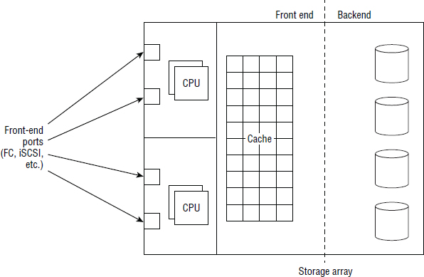
Let's get under the hood a little now. Figure 3.3 shows the major components of a storage array (the same as previously seen in Figure 3.2).
We'll start at the front end and work our way through the array, all the way to the backend (left to right on Figure 3.3).
Front End
The front end of a storage array is where the array interfaces with the storage network and hosts—the gateway in and out of the array, if you will. It is also where most of the magic happens.
If you know your SCSI, the front-end ports on a SAN storage array act as SCSI targets for host I/O, whereas the HBA in the host acts as the SCSI initiator. If your array is a NAS array, the front-end ports are network endpoints with IP addresses and Domain Name System (DNS) hostnames.
Ports and Connectivity
Servers communicate with a storage array via ports on the front, which are often referred to as front-end ports. The number and type of front-end ports depends on the type and size of the storage array. Large enterprise arrays can have hundreds of front-end ports, and depending on the type of storage array, these ports come in the following flavors: FC, SAS, and Ethernet (FCoE and iSCSI protocols).
Most high-end storage arrays have hot-swappable front-end ports, meaning that when a port fails, it can be replaced with the array still online and servicing I/O.
Hosts can connect to storage arrays in different ways, such as running a cable directly from the server to the storage array in a direct attached approach or connecting via a network. It is also possible to have multiple connections, or paths, between a host and a storage array, all of which need managing. Let's look more closely at each of these concepts.
Direct Attached
Hosts can connect directly to the front-end ports without an intervening SAN switch in a connectivity mode known as direct attached. Direct attached has its place in small deployments but doesn't scale well. In a direct attached configuration, there can be only a one-to-one mapping of hosts to storage ports. If your storage array has eight front-end ports, you can have a maximum of eight servers attached. In fact, as most people follow the industry-wide best practice of having multiple paths to storage (each host is connected to at least two storage array ports), this would reduce your ratio of hosts to storage ports from one-to-one to one-to-two, meaning that an eight-port storage array could cater to only four hosts—each with two paths to the storage array. That is not scalable by any stretch of the imagination.
SAN Attached
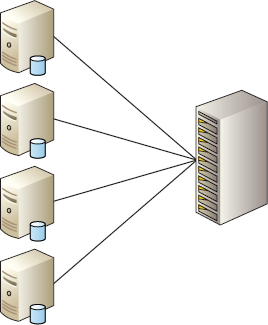
Far more popular and scalable than direct attached is SAN attached. SAN attached places a switch between the server and the storage array and allows multiple servers to share the same storage port. This method of multiple servers sharing a single front-end port is often referred to as fan-in because it resembles a handheld fan when drawn in a diagram. Fan-in is shown in Figure 3.4.
Multipath I/O
A mainstay of all good storage designs is redundancy. You want redundancy at every level, including paths across the network from the host to the storage array. It is essential that each server connecting to storage has at least two ports to connect to the storage network so that if one fails or is otherwise disconnected, the other can be used to access storage. Ideally, these ports will be on separate PCIe cards.
However, in micro server and blade server environments, a single HBA with two ports is deployed. Having a single PCIe HBA with two ports is not as redundant a configuration as having two separate PCIe HBA cards, because the dual-ported PCIe HBA is a single point of failure. Each of these ports should be to discrete switches, and each switch should be cabled to different ports on different controllers in the storage array. This design is shown in Figure 3.5.
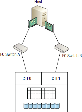
Host-based software, referred to as multipath I/O (MPIO) software, controls how data is routed or load balanced across these multiple links, as well as taking care of seamlessly dealing with failed or flapping links.
Common MPIO load-balancing algorithms include the following:
Failover Only Where one path to a LUN is active and the other passive, no load balancing is performed across the multiple paths.
Round Robin I/O is alternated over all paths.
Least Queue Depth The path with the least number of outstanding I/Os will be used for the next I/O.
All modern operating systems come with native MPIO functionality that provides good out-of-the-box path-failure management and load balancing. OS and hypervisor MPIO architectures tend to be frameworks that array vendors can write device-specific modules for. These device-specific modules add functionality to the host's MPIO framework—including additional load-balancing algorithms that are tuned specifically for the vendor's array.
Exercise 3.1 walks you through configuring MPIO load balancing.
EXERCISE 3.1
Configuring an MPIO Load-Balancing Policy in Microsoft Windows
The following procedure outlines how to configure the load-balancing policy on a Microsoft Windows server using the Windows MPIO GUI:
- Open the Microsoft Disk Management snap-in by typing diskmgmt.msc at the command line or at the Run prompt.
- In the Disk Management UI, select the disk you wish to set the load-balancing policy for, right-click it, and choose Properties.
- Click the MPIO tab.
- From the Select MPIO Policy drop-down list, choose the load-balancing policy that you wish to use.
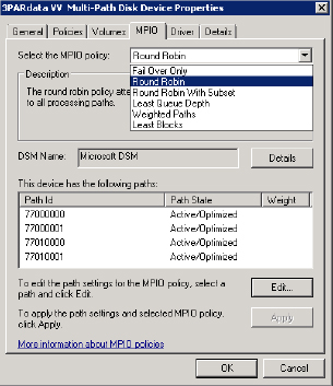
This graphic shows all four paths to this LUN as Active/Optimized, which tells us that this LUN exists on a grid architecture–based array. If it was a LUN on a dual-controller array that supported only ALUA, only one path would be Active/Optimized, and all other paths would be failover only.
The Microsoft Device Specific Module (DSM) provides some basic load-balancing policies, but a vendor-specific DSM may offer additional ones.
Some vendors also offer their own multipathing software. The best example of this is EMC PowerPath. EMC PowerPath is a licensed piece of host-based software that costs money. However, it is specifically written to provide optimized multipathing for EMC arrays. It also provides the foundation for more-advanced technologies than merely MPIO.
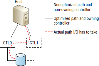
Using MPIO for dual-controller arrays that support only ALUA requires that multiple paths to LUNs be configured as failover only, ensuring that only the path to the active controller (the controller that owns the LUN) is used. Accessing a LUN over a nonoptimized path (a path via the controller that does not own the LUN) can result in poor performance over that path. This is because accessing a LUN over a nonoptimized path results in the I/O having to be transferred from the controller that does not own the LUN, across the controller interconnects, to the controller that does own it. This incurs additional latency. This is depicted in Figure 3.6.
Front-End Port Speed
Front-end ports can usually be configured to operate at a few different speeds, depending on the type of front-end port they are. For example, a 16 Gbps FC front-end port can usually be configured to operate at 16 Gbps, 8 Gbps, or 4 Gbps. In a Fibre Channel SAN, it is always a good idea to hard-code the port speed and not rely on the autonegotiate protocol. When doing this, make sure you hard-set the ports at either end of the cable to the same speed. This will ensure the most reliable and stable configuration. However, Ethernet-based storage networks should use the autonegotiate (AN) setting and should not hard-code port speeds.
CPUs
Also key to the front end are the CPUs. CPUs, typically Intel, are used to power the front end. They execute the firmware (often called microcode by storage people) that is the brains of the storage array. Front-end CPUs, and the microcode they run, are usually responsible for all of the following:
- Processing I/O
- Caching
- Data integrity
- Replication services
- Local copy services
- Thin provisioning
- Compression
- Deduplication
- Hypervisor and OS offloads
It is not uncommon for large, enterprise-class storage arrays to have about 100 front-end CPUs in order to both increase the front-end processing power and provide redundancy. It is also common for smaller, low-end storage arrays to have very few CPUs and use the same CPUs to control the front end and the backend of an array.
Vendors are keen to refer to their storage arrays as intelligent. While that is a bit of a stretch and a bit of an insult to anything truly intelligent, if there is any intelligence in a storage array, that intelligence resides in the firmware that runs the array.
As mentioned, the term microcode is frequently used in the storage industry to refer to the software/firmware that is the brains of a storage array. You may also see the term shortened it to ucode. Technically speaking, this should really be written as μcode (the symbol μ is the SI symbol for micro) but as the μ symbol doesn't appear on any standard QWERTY keyboard, it is easier to substitute the letter u for it. Long story short, the term ucode refers to the microcode that runs the array. It is pronounced you-code.
Because the firmware is the brains of the array, you'd be right in thinking that firmware management is crucial to the stability and performance of any storage array. If you don't bother keeping it up-to-date, you will fall out of vendor support and put yourself at risk when issues arise. You really can't afford to put your storage in jeopardy by not keeping your firmware up-to-date.
On the other hand, you probably don't want to be on the hemorrhaging edge of firmware technology. Running the very latest version of firmware the day it is released (or heaven forbid, a prerelease version) in your production environment massively increases your risk of encountering bugs, which at best wastes time and money, and at worst can temporarily cripple your organization. A good rule of thumb is to wait a minimum of three months after general availability (GA) before dipping your toe into the latest and greatest firmware revision from a vendor.
It is also a good idea to methodically deploy new firmware to your estate. A common approach is as follows:
- LAB. Deploy in the lab first and run for at least a month, testing all of your configuration, including testing failure scenarios and rebooting attached servers.
- DEV. Deploy to your development environment and run for at least a month.
- DR. Deploy to your disaster recovery (DR) arrays (if you operate a live/DR environment) and run for one week.
- PROD. Deploy to your live production arrays.
Obviously, this list will have to be tweaked according to your environment, as not everyone has the luxury of a fully functional lab, development environment, and so on. However, here are a few points worth noting:
- Let somebody else find the bugs. This is the main reason for allowing the code to mature in the wild for three months before you take it. Usually within three months of deployment, people have uncovered the worst of the bugs. It also allows the vendor time to patch anything major.
- Do not deploy directly to your live production environment. You want to give yourself a fighting chance of weeding out any potential issues in your less-mission-critical environments.
- If you replicate between storage arrays, it is usually not a great idea to have them running different versions of firmware for very long. It is usually a good idea to upgrade the DR array one weekend and then upgrade the live production array the following weekend. However, if you do not have a lab or development environment to soak test in first, it may be a better idea to run in DR for two to four weeks before upgrading live production arrays.

Always check with your vendor that you are upgrading via a supported route. Some vendors will not allow you to run different versions of code on arrays that replicate to each other. The preceding rules are guidelines only, and you need to engage with your vendor or channel partner to ensure you are doing things by the book.
An obvious reason to circumvent the preceding rules is if the new version of code includes a major bug fix that you are waiting for.
Another thing to be aware of is that many organizations standardize on an annual firmware upgrade plan. Upgrading annually allows you to keep reasonably up-to-date and ensures you don't fall too far behind.
One final point worth noting on the topic of firmware management is to ensure that you understand the behavior of your array during a firmware upgrade. While most firmware upgrades these days tend to be NDUs, you need to check. The last thing you want to do is upgrade the firmware only to find out halfway through that all front-end ports will go offline part way through the upgrade, or an entire controller will go offline for a while, lowering the overall performance capability of the array during the upgrade!
LUNs, Volumes, and Shares
Disks are installed on the backend, and their capacity is carved into volumes by the array. If your storage array is a SAN array, these volumes are presented to hosts via front-end ports as LUNs. Rightly or wrongly, people use the terms volume and LUN interchangeably. To the host that sees the LUN, it looks and behaves exactly like a locally installed disk drive. If your array is a NAS array, these volumes are presented to hosts as network shares, usually NFS or SMB/CIFS.
LUNs on a storage array are usually expandable, meaning you can grow them in size relatively easily. There are sometimes a few complications such as replicated LUNs, but this shouldn't be an issue on any decent storage array. If it is, you are buying something ancient.
Reducing the size of a LUN, on the other hand, is far more dangerous. For this reason, it is almost never performed in block-storage environments where the storage array has no knowledge of the filesystem on the LUN. However, NAS arrays have the upper hand here, as they own both the filesystem and the volume. Knowledge truly is power, and it is common to see good NAS arrays offer the ability to shrink volumes.
LUN Masking
As a security precaution, all LUNs presented out of a SAN storage array should be masked on the array. LUN masking is the process of controlling which servers can see which LUNs. Actually, it is the process of controlling which HBAs can see which LUNs. It is basically access control. Without LUN masking, all LUNs presented out of the front of a storage array would be visible to all connected servers. As you can imagine, that would be a security and data-corruption nightmare.
These days, LUN masking is almost always performed on the storage array—using the World Wide Port Name (WWPN) of a host's HBA in FC environments, and using the IP address or iSCSI Qualified Name (IQN) in iSCSI environments. For example, on a storage array, you present LUNs on a front-end port. That port has an access control list on it that determines which host HBA WWPNs are allowed to access which LUNs. With LUN masking enabled, if your host's HBA WWPN is not on the front-end port's access control list, you will not be able to see any LUNs on that port. It is simple to implement and is standard on all storage arrays. Implement it!
![]() Real World Scenario
Real World Scenario
The Importance of Decommissioning Servers Properly
A common oversight in storage environments is not cleaning up old configurations when decommissioning servers. Most companies will at some point have decommissioned a server and then rebuilt it for another purpose, but will have not involved the storage team in the decom process. When the server is rebuilt and powered up, it can still see all of its old storage from its previous life. This is because the server still has the same HBA cards with the same WWPNs, and these WWPNs were never cleared up from the SAN zoning and array-based LUN masking. In most cases, this is a minor annoyance, but it can be a big problem if the server used to be in a cluster that had access to shared storage!
Back in the day, people used to apply masking rules on the host HBA as well. In modern storage environments, this is rarely if ever done anymore. One of the major reasons is that it was never a scalable solution. In addition, this provided little benefit beyond performing LUN masking on the storage array and SAN zoning in the fabric. Exercise 3.2 discusses how to configure LUN masking.
EXERCISE 3.2
Configuring LUN Masking
The following step-by-step example explains a common way to configure LUN masking on a storage array. The specifics might be different depending on the array you are using. In this example, you will configure a new ESX host definition for an ESX host named legendary-host.nigelpoulton.com.
- Create a new host definition on the array.
- Give the host definition a name of legendary-host. This name can be arbitrary but will usually match the hostname of the host it represents.
- Set a host mode or host persona of Persona 11 - VMware. This is the persona type for an ESX host on an HP 3PAR array and should be used for all ESX host definitions. The value will be different on different array technologies.
- Add the WWPNs of the HBAs in legendary-host to the host definition. legendary-host is configured on your array, and you can now map volumes to it.
The next steps will walk you through the process of mapping a single 2 TB volume to legendary-host:
- Select an existing 2 TB volume and choose to export this volume to a host.
- Select legendary-host as the host that you wish to export the volume to.
Once you have completed these procedures, a 2 TB volume will be exported to legendary-host (actually the HBA WWPNs configured as part of the legendary-host host definition in step 4). No other hosts will be able to access this volume, as the ACL on the array will allow only initiators with the WWPNs defined in step 4 to access the LUN.
The equivalent of LUN masking in the NAS world is restricting the IP address or host-name to which a volume/share is exported. Over and above that, you can also implement file and folder permissions.
LUN Sharing
While it is possible for multiple hosts to access and share the same block LUN, this should be done with extreme care! Generally speaking, the only time multiple servers should be allowed to access and write to the same shared LUN is in cluster configurations in which the cluster is running proper clustering software that ensures the integrity of the data on the LUN—usually by ensuring that only a single server can write to the LUN at any one time.
Certain backup software and designs may require the backup media server to mount a shared LUN as read-only so that it can perform a backup of the data on a LUN. But again, the backup software will be designed to do this.
If two servers write to the same LUN without proper clustering software, the data on the LUN will almost certainly become corrupt.
Exercise 3.3 examines how to provision a LUN to a cluster.
EXERCISE 3.3
LUN Presentation in a Cluster Configuration
This exercise walks you through provisioning a single 2 TB LUN to an ESX cluster that contains two ESX hosts named ESX-1 and ESX-2. These two hosts are already defined on the array.
- Create a new host set definition on the array. A host set is a host group that can contain multiple host definitions.
- Give the host set a name of legendary-ESX-cluster.
- Add the ESX-1 and ESX-2 hosts to the host set. The host set legendary-ESX-cluster is now configured on your array and contains two ESX hosts and their respective WWPNs.
The next step is to map your 2 TB volume to the host set.
- Select an existing 2 TB volume and choose to export this volume to a host set.
- Select legendary-ESX-cluster as the host set that you wish to export the volume to.
The 2 TB volume is now presented to ESX hosts ESX-1 and ESX-2. Both ESX hosts can now access this volume.
Thick and Thin LUNs
LUNs on a storage array can be thick or thin. Traditionally, they were always thick, but these days, more often than not they are thin. We will discuss thick and thin LUNs later in the chapter, in the “Thin Provisioning” section.
Cache
It could be said that the cache is the heart of a storage array. It is certainly the Grand Central Station of an array. On most storage arrays, everything has to pass through cache. All writes to the array go to cache first before being destaged to the backend disk at a later time. All reads from the array get staged into cache before being sent to the host. Even making a clone of a volume within a single array requires the blocks of data to be read from the backend, into cache, and then copied out to their new locations on the same backend. This all means that cache is extremely important.
Cache is also crucial to flash-based storage arrays, but they usually have less of it, as the backend is based on solid-state media so there isn't such a desperate need for a performance boost from cache. Flash-based storage arrays tend to use DRAM cache more for metadata caching and less for user data caching.
Performance Benefits of Cache
The raison d'etre of cache in a spinning-disk-based storage array is to boost performance. If an I/O can be satisfied from cache, without having to go to the disk on the backend, that I/O will be serviced hundreds of times more quickly! Basically, a well-implemented cache hides the lower performance of mechanical disks behind it.
In relation to all-flash arrays, DRAM cache is still faster than flash and can be used in a similar way, only the straight performance benefits are not as apparent.
It is necessary for write I/O to come into a storage array and be protected in two separate cache areas before an acknowledgment (ACK) can be issued to the host. That write I/O is then destaged to the backend at a later point in time. This behavior significantly improves the speed of ACKs. This modus operandi is referred to as write-back caching. If there are faults with cache, to the extent that incoming writes cannot be mirrored to cache (written to two separate cache areas), the array will not issue an ACK until the data is secured to the backend. This mode of operation is referred to as write-through mode and has a massively negative impact on the array's write performance, reducing it to the performance of the disks.
While on the topic of performance and write-through mode, it is possible to overrun the cache of a storage array, especially if the backend doesn't have enough performance to allow data in cache to be destaged fast enough during high bursts of write activity. In these scenarios, cache can fill up to a point generally referred to as the high write pending watermark. Once you hit this watermark, arrays tend to go into forced flush mode, or emergency cache destage mode, where they effectively operate in cache write-through mode and issue commands to hosts, forcing them to reduce the rate at which they are sending I/O. This is not a good situation to be in!
Read Cache and Write Cache
Cache memory for user data is also divided into read and write areas. Arrays vary in whether or not they allow/require you to manually divide cache resources into read cache and write cache. People tend to get religious about which approach is best. Let the user decide or let the array decide. I prefer the approach of letting the array decide, as the array can react more quickly than I can, as well as make proactive decisions on the fly, based on current I/O workloads. I do, however, see the advantage of being able to slice up my cache resources on smaller arrays with specific, well-known workloads. However, on bigger arrays with random and frequently changing workloads, I would rather leave this up to the array.
On the topic of mirroring cache: it is common practice to mirror only writes to cache. Read cache doesn't need mirroring, as the data already exists on protected disk on the backend, and if the cache is lost, read data can be fetched from the backend again. If the read cache is mirrored, it unnecessarily wastes precious cache resources.
Data Cache and Control Cache
High-end storage arrays also tend to have dedicated cache areas for control data (metadata) and dedicated areas for user data. This bumps up cost but allows for higher performance and more-predictable cache performance. Disk-based storage arrays are addicted to cache for user data performance enhancement as well as caching metadata that has to be accessed quickly. All-flash arrays are less reliant on cache for user data performance enhancements but still utilize it extensively for metadata caching.
Cache Hits and Cache Misses
A cache hit occurs for a read request when the data being requested is already available in cache. This is sometimes called a read hit. Read hits are the fastest types of read. If the data does not exist in cache and has to be fetched from the backend disk, then a cache miss, or read miss, is said to have occurred. And read misses can be shockingly slower than read hits. Whether or not you get a lot of read hits is highly dependent on the I/O workload. If your workload has high referential locality, you should get good read hit results.
Referential locality refers to how widely spread over your address space your data is. A workload with good referential locality will frequently access data that is referentially close, or covers only a small area of the address space. An example is a large database that predominantly accesses only data from the last 24 hours.
For write operations, if cache is operating correctly and an ACK can be issued to a host when data is protected in cache, this is said to be a cache hit. On a fully functioning array, you should be seeing 100 percent cache write hit stats.
Protecting Cache
As cache is so fundamental to the smooth operation of an array, it is always protected—usually via mirroring and batteries. In fact, I can't remember seeing an array pathetic enough not to have protected/mirrored cache.
There are various ways of protecting cache, and mirroring is the most common. There is more than one way to mirror cache. Some ways are better than others. At a high level, top-end arrays will take a write that hits a front-end port and duplex it to two separate cache areas in a single operation over a fast internal bus. This is fast. Lower-end systems will often take a write and commit it to cache in one controller, and then, via a second operation, copy the write data over an external bus, maybe Ethernet, to the cache in another controller. This is slower, as it involves more operations and a slower external bus.
As well as mirroring, all good storage arrays will have batteries to provide power to the cache in the event that the main electricity goes out. Remember that DRAM cache is volatile and loses its contents when you take away the power. These batteries are often used to either provide enough power to allow the array to destage the contents of cache to the backend before gracefully powering down, or to provide enough charge to the cache Dual Inline Memory Modules (DIMMs) to keep their contents secure until the power is restored.
As I've mentioned mirroring of cache, it is worth noting that only writes should be mirrored to cache. This is because read data already exists on the backend in protected nonvolatile form, so mirroring reads into cache would be wasteful of cache resources.
Protecting cache by using batteries is said to make the cache nonvolatile. Nonvolatile cache is often referred to as nonvolatile random access memory (NVRAM).
Cache Persistence
All good high-end storage arrays are designed in a way that cache DIMM failures, or even controller failures, do not require the array to go into cache write-through mode. This is usually achieved by implementing a grid architecture with more than two controllers. For example, a four-node array can lose up to two controller nodes before no longer being able to mirror/protect data in cache. Let's assume this four-controller node array has 24 GB of cache per node, for a total of 96 GB of cache. That cache is mirrored, meaning only 48 GB is available for write data. Now assume that a controller node dies. This reduces the available cache from 96 GB to 72 GB. As there are three surviving controllers, each with cache, writes coming into the array can still be protected in the cache of multiple nodes. Obviously, there is less overall available cache now that 24 GB has been lost with the failed controller, but there is still 36 GB of mirrored cache available for write caching.
This behavior is massively important, because if you take the cache out of a storage array, especially a spinning-disk-based storage array, you will find yourself in a world of pain!
Common Caching Algorithms and Techniques
While you don't need to know the ins and outs of caching algorithms to be a good storage pro, some knowledge of the fundamentals will hold you in good stead at some point in your career.
Prefetching is a common technique that arrays use when they detect sequential workloads. For example, if an array has received a read request for 2 MB of contiguous data to be read from the backend, the array will normally prefetch the next set of contiguous data into cache, based on there being a good probability that the host will ask for that. This is especially important on disk-based arrays, as the R/W heads will already be in the right position to fetch this data without having to perform expensive backend seek operations. Prefetching is far less useful on all-flash arrays, as all-flash arrays don't suffer from mechanical and positional latency as spinning disk drives do.
Most arrays also operate some form of least recently used (LRU) queuing algorithm for data in cache. LRUs are based on the principle of keeping the most recently accessed data in cache, whereas the data least recently accessed will drop out of cache. There is usually a bit more to it than this, but LRU queues are fundamental to most caching algorithms.
Flash Caching
It is becoming more and more popular to utilize flash memory as a form of level 2 (L2) cache in arrays. These configurations still have an L1 DRAM cache but augment it with an additional layer of flash cache.
Assume that you have an array with a DRAM cache fronting spinning disks. All read requests pull the read data into cache, where it stays until it falls out of the LRU queue. Normally, once this data falls out of the LRU queue, it is no longer in cache, and if you want to read it again, you have to go and fetch it from the disks on the backend. This is sloooow! If your cache is augmented with an L2 flash cache, when your data falls out of the L1 DRAM cache, it drops into the L2 flash cache. And since there's typically a lot more flash than DRAM, the data can stay there for a good while longer before being forgotten about and finally evicted from all levels of array cache. While L2 flash caches aren't as fast as L1 DRAM caches, they are still way faster than spinning disk and can be relatively cheap and large! They are highly recommended.
Flash cache can be implemented in various ways. The simplest and most crude implementation is to use flash Solid State Drives (SSD) on the backend and use them as an L2 cache. This has the performance disadvantage that they live on the same shared backend as the spinning disks. This places the flash memory quite far from the controllers and makes access to them subject to any backend contention and latency incurred by having to traverse the backend. Better implementations place the L2 flash cache closer to the controllers, such as PCIe-based flash that is on a PCIe lane on the same motherboard as the controllers and L1 DRAM cache.
External Flash Caches
Some arrays are now starting to integrate with flash devices installed in host servers. These systems tend to allow PCIe-based flash resources in a server to be used as an extension of array cache—usually read cache.
They do this by various means, but here is one method: When a server issues a read request to the array, the associated read data is stored in the array's cache. This data is also stored in the PCIe flash memory in the server so that it is closer to the host and does not have to traverse the storage network and be subject to the latency incurred by such an operation. Once in the server's PCIe flash memory, it can be aged out from the array's cache. This approach can work extremely well for servers with read-predominant workloads.
Lots of people like to know as much about array cache as they can. Great. I used to be one of them. I used to care about slot sizes, cache management algorithms, the hierarchical composition of caches, and so on. It is good for making you sound like you know what you're talking about, but it will do you precious little good in the real world! Also, most storage arrays allow you to do very little cache tuning, and that's probably a good thing.
Backend
The backend of a storage array refers to the drives, drive shelves, backend ports, and the CPUs that control them all.
CPUs
High-end enterprise storage arrays usually have dedicated CPUs for controlling the backend functions of the array. Sometimes these CPUs are responsible for the RAID parity calculations (XOR calcs), I/O optimization, and housekeeping tasks such as drive scrubbing. Mid- to low-end arrays often have fewer CPUs and as a result front-end and backend operations are controlled by the same CPUs.
Backend Ports and Connectivity
Backend ports and connectivity to disk drives are predominantly SAS these days. Most drives on the backend have SAS interfaces and speak the SAS protocol. Serial Advanced Technology Attachment (SATA) and FC drives used to be popular but are quickly being replaced by SAS.
99 percent of the time you shouldn't need to care about the protocol and connectivity of the backend. The one area in which FC had an advantage was if there was no space to add more disk shelves in the data center near the array controllers. FC-connected drives allowed you to have your drives several meters away from the controllers, in a different aisle in the data center. However, this was rarely implemented.
![]() Real World Scenario
Real World Scenario
The Importance of Redundancy on the Backend
A customer needed to add capacity to one of their storage arrays but had no free data-center floor space adjacent to the rack with the array controllers in it. As their backend was FC based, they decided to install an expansion cabinet full of disk drives in another row several meters away from the controllers. This worked fine for a while, until the controllers suddenly lost connectivity to the disks in the expansion cabinet placed several meters away from the controller cabinet.
It turned out that a data-center engineer working under the raised floor had dropped a floor tile on an angle and damaged the FC cables connecting the controllers to the disk drive shelves. This took a long time to troubleshoot and fix, and for the duration of the fix time, the array was down. This could have been avoided by running the cables via diverse routes under the floor, but in this case this was not done. The array was taken out of action for several hours because of bad cabling and a minor data-center facilities accident.
Drives
Most drives these days, mechanical and flash, are either SATA or SAS based. There is the odd bit of FC still kicking around, but these drives are old-school now. SAS is increasingly popular in storage arrays, especially high-end storage arrays because they are dual-ported, whereas SATA is still popular in desktop and laptop computers.
Drives tend to be the industry standard 2.5-inch or 3.5-inch form factor, with 2.5-inch becoming more and more popular. And backend drives are always hot-swappable!
The backend, or at least the data on the backend, should always be protected, and the most common way of protecting data on the backend is RAID. Yes, RAID technology is extremely old, but it works, is well-known, and is solidly implemented. Most modern arrays employ modern forms of RAID such as network-based RAID and parallelized RAID. These tend to allow for better performance and faster recovery when components fail.
Most modern arrays also perform drive pooling on the backend, often referred to as wide striping. We cover this in more detail later in the chapter.
Power
Just about every storage array on the market will come with dual hot-swap power supplies. However, high-end arrays take things a bit further. Generally speaking, high-end storage arrays will take multiple power feeds that should be from separate sources, and tend to prefer UPS-fed three-phase power. They also sport large batteries that can be used to power the array if there is loss of power from both feeds. These batteries power the array for long enough to destage cache contents to disk or flash, or alternatively persist the contents of cache for long periods of time (one or two days is common).
Storage Array Intelligence
Yes, the term intelligence is a bit of a stretch, but some of this is actually starting to be clever stuff, especially the stuff that integrates with the higher layers in the stack such as operating systems, hypervisors, and applications.
Replication
In this book, replication refers specifically to remote replication. The raison d'etre of replication is to create remote copies (replicas) of production data. Say you have a mission-critical production database in your New York data center that you wish to replicate to your Boston data center so you have an up-to-date copy of your data in Boston in case your production systems go down in New York. Replication is what you need for this.
These copies, sometimes called replicas, can be used for various things, but more often than not they are used for the following:
- Providing business continuity in the event of local outages, as just described
- Test and development purposes, such as testing new models and queries against real data in an isolated environment, where they cannot impact production systems or change production data
Business Continuity
Data replication is only one component in a robust business continuity (BC) plan. It is also absolutely vital that business continuity plans are regularly tested. You do not want the first time you use your business continuity plan to be in the middle of a live disaster—hoping it will be all right on the same night. Chances are it won't!
Rehearsals are absolutely vital in managing effective business continuity plans. Test them and test them again!
Before you look into the types of replication, it is worth pointing out that most replication technologies cannot help with recovering from logical corruption such as a virus or deleted data. This is because the corruption itself (virus or deletion) will be replicated to the target array. Backups and snapshots are what you need to recover from logical corruption!
Array-Based Replication
In array-based replication, the storage array controls the replication of the data. One advantage is that the heavy lifting of the replication management is handled by the storage array, so no overhead is placed on your application servers. The downside is that the storage array does not understand applications—storage array-based replication is therefore not intelligent. This means that the replicated data at the remote site may not be in an ideal state for a clean and reliable application recovery and that more data may be sent across the replication link than if application-based replication were used. Obviously, this is extremely important. For this reason, array-based replication is losing ground to the increasingly popular application-based replication.
Array-based replication almost always requires the same kind of array at both ends of the link. For example, you couldn't replicate between an EMC VMAX array in Boston and a NetApp FAS in New York.
Application-Based Replication
Application-based replication does not use storage array-based replication technologies. First, this means that the overhead of replicating data is levied on the application servers. This may not be ideal, but most systems these days have enough CPU power and other resources to be able to cope with this.
The second, and far more important, fact about application-based replication is that it is application aware, or intelligent. This means it understands the application, replicates data in a way that the application likes, and ensures that the state of the replicated copy of data is in an ideal state for the application to use for a quick and smooth recovery.
Popular examples include technologies such as Oracle Data Guard and the native replication technologies that come with Microsoft technologies such as Microsoft SQL Server and Microsoft Exchange Server.
Host-Based and Hypervisor-Based Replication
Some logical volume managers and hypervisors are starting to offer better replication technologies, and they come in various forms. Some forms of host/hypervisor-based replication technologies are neither application nor storage array aware. They simply provide the same unintelligent replication offered by storage arrays but without offloading the burden of replication to the storage array. This is not the best scenario, but it is often cheap.
There are also hypervisor-based technologies that either perform replication or plug into storage array replication technologies. An example of hypervisor-based replication technologies is VMware vSphere Replication, which is managed by VMware Site Recovery Manager.
SRM is also storage-array-based replication aware and can be integrated with array-based replication technologies. It allows the array to perform the heavy lifting work of replication but integrates this with the ability of SRM to plan and manage site failovers.
Of the two options with VMware SRM, the built-in vSphere replication is a new technology and is potentially more suited to smaller environments, whereas the option to integrate SRM with array-based replication technologies is considered more robust and scalable.
These types of replication technology are becoming increasingly popular. Beware, though. They can sometimes require both storage array replication licenses and hypervisor software licenses!
Synchronous Replication
Synchronous replication guarantees zero data loss. Great! I'm sure we all want that. However, there's always small print, and this time the small print says that synchronous replication comes with a performance cost.
Synchronous replication technologies guarantee zero data loss by making sure writes are secured at the source and target arrays before an ACK is issued to the application and the application considers the write committed. That is simple. Sadly, waiting for the write to complete at the target array can often incur a significant delay. The exact amount of delay depends on a few things, but it usually boils down to the network round-trip time (RTT) between the source and target arrays. Network RTT is also generally proportional to the distance between the source and target arrays.
Figure 3.7 shows a storyboard of array-based synchronous replication.
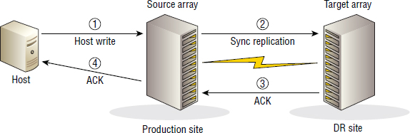
Because synchronous replication offers zero data loss, this gives a recovery point objective (RPO) of zero. At a high level, RPO is the amount of data that can be lost, measured in time units. For example, an RPO of 10 minutes means that the data used to recover an application or service can be a maximum of 10 minutes out-of-date at the time the data loss occurred. Therefore, RPOs dictate the business continuity technologies used to protect business data. For example, a daily backup of an application is no use if the RPO for that application is 1 hour.
Replication Distances and Latency
As a very loose ballpark figure, a distance of 75 miles between source and target arrays may incur an RTT of 1–2 milliseconds (ms). That is 1–2 ms of latency that would not be incurred if you were not synchronously replicating your data.
While on the topic of distances, a good ballpark figure for maximum distance you might want to cover in a synchronous replication configuration might be ∼100 miles. However, it is important that you consult your array vendor over things like this, as they may impose other limitations and offer recommendations depending on their specific technology. This is not something you want to design on your own and get wrong.
Make sure that you include the array vendor as well as the network team when dealing with site-to-site replication links.
Always make sure that when referring to the distance between data centers, you are indicating the route taken by the network and not the distance if travelling by car. The distance could be 60 miles by car but a lot longer via the route the network takes.
It is also important to be able to test and guarantee the latency of the link. You may want to get latency guarantees from your Wide Area Network (WAN) provider.
Replication Link Considerations
When deploying synchronous replication, you should also be savvy to the importance of the network links connecting your source and target arrays. A flaky link that is constantly up and down will mean that your solution cannot guarantee zero data loss without stopping writes to the application while the network link is down. Most organizations will allow writes to the application to continue while replication is down; however, for the duration of the replication outage, the remote replica will be out of sync. If you lose the primary copy while replication is down, your replica at the remote site will not be up-to-date, your Service Level Agreement (SLA) will be broken, and you will be facing a data-loss scenario if you need to bring the applications up in DR.
Although rare, some organizations do have applications that they fence off (stop writing to) if the remote replica cannot be kept in sync. These tend to be special-case applications.
Because of all of this, it is important to have multiple, reliable, diverse replication links between your sites. All tier 1 data centers will be twin tailed—two links between sites that each take diverse routes.
You will also want to consider the sizing of your replication link. If you do not size your link to be able to cope with your largest bursts of traffic, the link will be saturated when you experience high bursts of write data, and subsequently the performance of your applications will drop. Some organizations are happy to take this on the chin, as it means they don't have to oversize their replication links to deal with peak traffic. The important thing is that you know your requirements when sizing and speccing replication links. Figure 3.8 shows network bandwidth utilization at hourly intervals. In order for this solution to ensure that the remote replica does not lag behind the production source volume, the network link will need to be sized to cope with peak traffic.
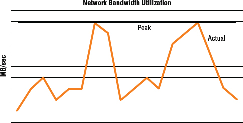
Asynchronous Replication
The major difference between synchronous and asynchronous replication is that with asynchronous replication, each write is considered complete when the local array acknowledges it. There is no wait for the write to be committed to the replica volume before issuing the ACK.
This means several things.
First, asynchronous does not provide zero data loss. In fact, asynchronous replication guarantees to lose data for you! How much data is lost depends entirely on your configuration. For example, if your replication solution replicates only every 5 minutes, you could lose slightly more than 5 minutes’ worth of data.
Next, and somewhat more positively, asynchronous replication does not incur the performance penalty that synchronous replication does. This is because the write to the remote array is done in a lazy fashion at a later time.
It also means that the distances between your source and target array can be much larger than in synchronous configurations. This is because the RTT between the source and target array no longer matters. You can theoretically place your source and target arrays at opposite ends of the planet.
There is also no need to spec your network connections between sites to cater for peak demand. However, you should still spec your network link so that you don't slip outside of your agreed RPO.
All of this is good, assuming you can sleep at night knowing you will lose some data if you ever have to invoke DR.
Invoking DR (disaster recovery) refers to bringing an application up by using its replicated storage. This usually involves failing the application—including the server, network, and storage—over to the standby server, network, and storage in the remote disaster recovery data center.
Storage arrays tend to implement asynchronous replication, shown in Figure 3.9, in one of two ways:
- Snapshot based
- Journal based
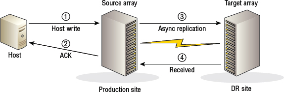
The difference to note between Figure 3.9 and Figure 3.7 is that the host receives an ACK—and can therefore continue issuing more I/O—after step 2 in Figure 3.9.
Snapshot-Based Asynchronous Replication
In snapshot-based asynchronous replication, the source array takes periodic point-in-time snapshots of the source volume and then replicates the snapshot data over the wire to the target array, where it is applied to the replica volume.
This type of replication is schedule based, meaning that you schedule the snaps and replication interval according to your required recovery point objective (RPO). Assume you have agreed to an SLA with the business to be able to recover data to within 10 minutes of the time at which an incident occurred. Configuring a replication interval of 5 minutes will meet that RPO and ensure that the replica volumes never lag more than ∼5 minutes behind the source volumes.
Good storage arrays have an interface that allows you to specify your RPO, and it will configure the replication specifics for you to ensure that your RPO SLA is met. Better storage arrays are RPO driven to even greater depths. For example, if you have some volumes configured for a 15-minute RPO and others for a 20-minute RPO, if the array encounters replication congestion, the array will prioritize replication based on which RPOs are closest to breaking. That borders on array intelligence!
If your storage array is stuck in the '90s and doesn't understand RPOs and SLAs, you will have to manually consider these things when configuring replication.
Be careful. An RPO of 10 minutes does not mean you can configure a replication update interval of 10 minutes! This is essentially because your snapshot data won't instantly arrive at the target array the moment it is sent. It takes time for data to be transmitted across a network, and often the wire used for asynchronous replication is a relatively cheap, low-bandwidth wire. Assuming it take 2 minutes for all your data to arrive at the target array, that is potentially a 12-minute RPO, not a 10-minute one.
Usually, if your array supports snapshot-based asynchronous replication, that array will use the same snapshot engine that it uses to take local snapshots. Depending on your array, this can mean that replication-based snapshots eat into the maximum number of snapshots supported on the array. So if your array supports a maximum of 1,024 snapshots, and you are replicating 256 volumes by using snapshot-based asynchronous replication, you have probably eaten 256 of the array's maximum 1,024 snaps.
With snapshot-based asynchronous replication, beware of snapshot extent size—the granularity at which snapshots are grown. If the snapshot extent size is 64 KB, but all that you update between replication intervals is a single 4 KB block, what will actually be replicated over the wire is 64 KB—a single snapshot extent. No big deal, right? Now assume several large arrays sharing a remote replication link, each using snapshot-based replication. You update 1,000 unique 4 KB blocks and assume that this will replicate just under 4 MB of data across the wire. However, each of these 4 KB updates was in a unique extent on each volume, meaning that you will end up replicating 1,000 × 64 KB instead of 1,000 × 4 KB. The difference is then pretty large—62.5 MB instead of 3.9 MB!
A good thing about snapshot-based replication is that as long as your array has decent snapshot technology, it will coalesce writes. This means that if your app has updated the same data block 1,000 times since the last replication interval, only the most recent update of that data block will be sent across the wire with the next set of deltas, rather than all 1,000 updates.
Journal-Based Asynchronous Replication
Journal-based asynchronous replication technologies buffer write data to dedicated journal volumes, sometimes referred to as write intent logs. They have to be sized appropriately (usually oversized) in order to cope with large traffic bursts or times when the replication links are down. If you size these journal volumes too small, replication will break during large bursts or extended periods of the replication link downtime. On the other hand, if you size them too big, you're wasting space 99 percent of the time. It can be considered a balancing act or a dark art. Either way, it is quite complex from a design perspective.
When write I/Os come into the source array, they hit cache as usual, and the array issues the ACK to the host. The write I/O is also tagged with metadata to indicate that it is destined for a replicated volume, to ensure that the data is also asynchronously copied to the local journal volumes. The data is then destaged to disk as per standard cache destaging. At or around this time, the data is also written to the journal volume. From there, it is replicated to the target array at a time determined by the specifics of the array's replication technology. Generally speaking, though, journal-based replication does not lag very far behind the source volume.
Good arrays will apply write-sequencing metadata to the data buffered to the journal volumes so that proper write ordering is maintained when data is written to the target volume on the target array. Once the data is committed at the target array, it can be released from the journal volumes on the source array.
Implementations differ as to whether the source array pushes updates to the target array or whether the target array pulls the updates. For your day-to-day job, things like this should not concern you, certainly not as much as making sure you meet your SLAs and RPOs.
Although asynchronous replication doesn't require top-notch network bandwidth between source and target arrays, make sure your network connections aren't the runt of the network litter, relegated to feeding on the scraps left over after everyone else has had their share. If you don't give the links enough bandwidth, you will be operating outside your SLAs too often, risking not only your job but your company's data.
Figure 3.10 shows actual bandwidth utilization captured at hourly intervals, with an average line included. Asynchronous replication links do not need to be sized for peak requirements.
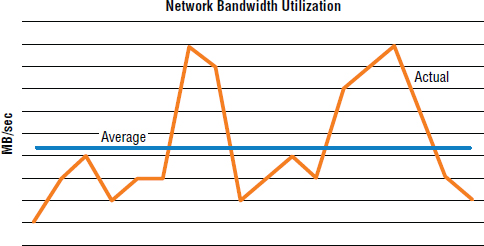
Replication Topologies
Depending on your array technology, various replication topologies are available. These can include more than two sites and utilize both synchronous and asynchronous replication technologies. It tends to be the higher-end, enterprise-class arrays that support the most replication topologies. The midrange arrays tend to support only more-basic topologies.
Three-Site Cascade
The three-site cascade replication topology utilizes an intermediate site, sometimes referred to as a bunker site, to connect the source array and the target array. Figure 3.11 shows an example of this topology.
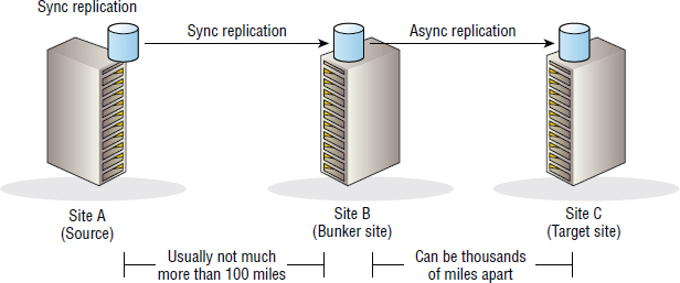
As shown in Figure 3.11, three-site cascade utilizes both synchronous and asynchronous replication—synchronous replication from the source site to the bunker site, and then asynchronous from the bunker site to the target site.
A major use case for three-site cascade topologies is to enable application recovery with zero data loss in the event of a localized issue in your primary data center that requires you to invoke disaster recovery plans. In this situation, you can bring your applications up in the bunker site with potentially zero data loss. However, if a major disaster renders both the primary data center and the bunker site inoperable, you have the third copy at the remote site. Because the replication between the bunker site and the target site is asynchronous, the distance can be large enough that even a major local disaster that affects the source and bunker sites will not affect the target site. And if a disaster big enough to affect the target site does occur, there is a good chance that recovering your company's applications will be the last thing on your mind!
Three-site cascade also allows your applications to remain protected even when the source site is down. This is because there are still two sites with replication links between them, and replication between these two sites can still operate.
The major weakness of the three-site cascade model is that the failure of the bunker site also affects the target site. Basically, if you lose the bunker site, your target site starts lagging further and further behind production, and your RPO becomes dangerously large.
This model is also used with the secondary array in the primary data center, rather than a remote bunker site, to protect against a failure of the primary array rather than a full site failure.
Three-Site Multitarget
The three-site multitarget topology has the source array simultaneously replicate to two target arrays. One target array is at a relatively close bunker site—close enough for synchronous replication. The other target is a long distance away and is replicated to asynchronously. This configuration is shown in Figure 3.12.
The major advantage that three-site multitarget has over three-site cascade is that the failure of the bunker site has no effect on replication to the target site. In this respect, it is more robust.
The major weakness of the three-site multitarget topology is that if the source site is lost, no replication exists between the bunker site and the target site. It can also place a heavier load on the primary array.
Three-Site Triangle
The three-site triangle topology is similar to three-site multitarget and offers all the same options, plus the addition of a standby replication link between the bunker and target site. Under normal operating circumstances, this additional link is not actively sending replication traffic, but can be enabled if the source site becomes unavailable. The three-site triangle topology is shown in Figure 3.13.
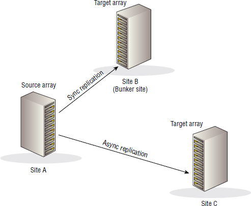
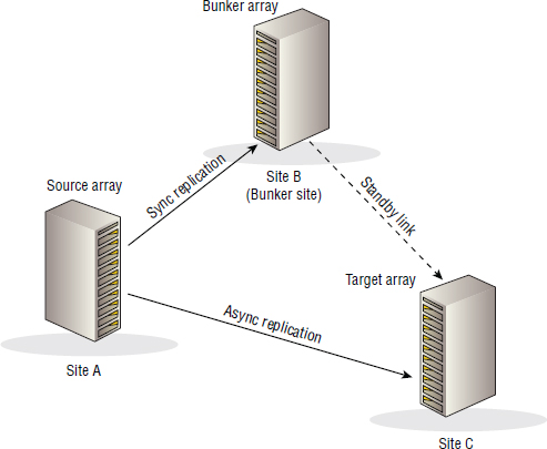
If the source site is lost, synchronizing replication between the bunker site and the target site does not require a full sync. The surviving arrays in the bunker and target site are able to communicate and determine which updates are missing at the target site, allowing for an incremental update from the bunker array to the target array. This allows you to get your application up and running again and have it protected by remote replication in a short period of time.
Not all storage arrays support all replication topologies. It is vital that you check with your array vendor or array documentation before assuming that your array supports a particular multisite replication topology.
Local Snapshots
Snapshots are nothing new, and in some cases neither is the technology behind them. Some snapshot implementations are ancient. We'll uncover some of these.
First, let's agree on our terminology: when referring to snapshots, I'm talking about local copies of data. And by local, I mean the snapshot exists on the same array as the source volume. Generally speaking, snapshots are point-in-time (PIT) copies.
These two facts—local and point-in-time—are the two major differences between local snapshots and remote replicas. Local snapshots are copies of production volumes created and maintained on the local array, whereas remote replicas are kept on a remote array. Also, local snapshots are point-in-time copies, whereas remote replicas are usually kept in sync, or semi-sync, with the primary production volume.
Finally, I use the terms source volume and primary volume to refer to the live production volume. And I use the term snapshot to refer to the point-in-time copy of the live production volume. This is shown in Figure 3.14.
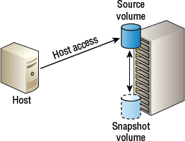
Snapshots and clones are created instantaneously, and depending on your array, snapshots and clones can be marked as read-only or read/write. All good arrays support read-only and read-write snapshots.
Snapshots are not backups! Take this statement, burn this into your brain, RAID protect it with at least double parity, and pin it to the high-performance cache of your brain so that it is always there for quick recall. Snapshots are not backups! Why? If you lose the RAID set, the array, or the site that hosts the primary volumes, you lose the snapshots as well. You do not want to be in this predicament.
Array-Based Snapshots
Two types of array-based snapshot technologies are commonly in use:
- Space-efficient snapshots
- Full clones
While they may go by various names, this book sticks to these two names. This section covers topics such as snapshot extent size, space reservation, the number of snapshots, how tiering can be used with snapshots, snapshot consistency, and the difference between copy-on-write and redirect-on-write snapshots.
Space-Efficient Snapshots
Space-efficient snapshots are generally pointer based. That tells you two important things:
Space efficient means that the snapshot contains only the parts of the primary volume that have changed since the snapshot was taken.
Pointer based means that none of the data that hasn't changed since the time of snapshot creation is copied to the snapshot. Instead, pointers point back to the data in the original volume for any data that hasn't changed since the time of snapshot creation.
Let's look at a quick and simple example with a figure or two.
Assume that you have a primary volume called LegendaryVol. LegendaryVol has 100 blocks numbered 0–99. At 1 p.m. on Monday, you make a space-efficient snapshot of LegendaryVol, at which point in time, all blocks in LegendaryVol are set to binary zero (0). Your snapshot is called LegendaryVol.snap. At the time you create the snapshot, LegendaryVol.snap consumes no space. If a host were to mount this snapshot and read its contents, all read I/O would be redirected back to the original data contained in LegendaryVol. All that LegendaryVol.snap consumes is pointers in memory that redirect read I/O back to the primary volume where the data exists.
Now let's assume that by 2 p.m. LegendaryVol has had blocks 0–9 updated to be binary ones (1). Any time a host wants to read data in LegendaryVol.snap, it will be redirected back to the source volume (LegendaryVol) except for reading blocks 0–9. This is because blocks 0–9 have changed in the primary volume, and in order to make sure that the snapshot looks exactly like the primary volume did at the point in time when the snap was taken (1 p.m.), the original contents were also copied to the snapshot.
So, at 2 p.m., the snapshot is still an exact image for how the primary volume was at 1 p.m.—all blocks are zeros. Job done. Also, the snapshot is space efficient because all unchanged data since the time the snapshot was created is still just pointers back to the original data, and the snapshot consumes only the space required to preserve the data that has changed since.
Full-Clone Snapshots
Full clones are not space efficient and therefore are not pointer based. They are, however, point-in-time copies of primary volumes.
At the time a full clone is created, an exact full copy of the primary volume is taken. This means that if the primary volume consumes 2 TB of storage at the time the clone was taken, each and every full clone of that volume will also consume 2 TB. This obviously means that full clones can be major consumers of disk space.
So why bother with full clones rather than space-efficient snapshots? There are a couple of common reasons:
- Reading and writing to a full clone has no direct impact on the primary volume. This is because the full clone is fully independent of the primary volume and contains no pointers. So you can hammer the clone with read and write requests, and this will have no impact on the performance of the primary volume. Snapshots, on the other hand, share a lot of data with their primary volumes, meaning that if you hammer the snapshot with intensive read and write I/O, you will be impacting the performance of the primary volume as well.
- Full clones are fully independent of the primary volumes from which they were created. This means that if the physical drives that the primary volume is on fail, the clone will not be impacted (assuming you don't make the mistake of keeping the primary and full clone on the same drives). In contrast, with snapshots, if the disks behind the primary volume fail, the snapshot will also be affected because of the way the snapshot just points back to the primary volume for much of its content.
In the modern IT world, where budgets are tight and ever shrinking, snapshots tend to be far more popular than full clones, so we'll spend a bit more time covering space-efficient snapshots.
Snapshot Extent Size
When it comes to space-efficient snapshots, size definitely matters. And bigger is not better!
If your array has a snapshot extent size (sometimes referred to as granularity) of 4 KB, it will be far more space efficient than an array with a snapshot granularity of 128 KB. Here is a quick example. Assume you make 100 changes to your primary volume since you created a snapshot. If your snapshot extent size is 4 KB, this will amount to a maximum of 400 KB consumed by your snapshot. On the other hand, if your snapshot extent size is 128 KB, the maximum space consumed by your snapshot just jumped up to 12,800 KB!
As another example, if you make a 4 KB update to a primary volume that has a snapshot, and the snapshot extent size is 128 KB, an additional 128 KB may have to be allocated to your snapshot. This is because the extent is the minimum unit of snapshot growth.
While this might not sound like the end of the world, consider the impact this has when you have lots of snaps and you are keeping them for long periods of time. This space inefficiency soon adds up. This also has an impact on how much data is sent over the wire in asynchronous replication configurations that are based on snapshots. So when it comes to snapshot granularity or extent size, smaller is definitely better.
Reserving Snapshot Space
On arrays based on legacy architectures, you are required to guess how much space your snapshots might consume, and then reserve that space up front! That's right, on day one you have to open up your wallet, and purchase and set aside space for potential snapshot use, space that might never be used. This type of architecture is made even worse by the fact that in many instances you have to prepare for the worst case and often end up ring-fencing far too much space. Legacy architectures like this are inexcusable in the modern IT world. Unfortunately, legacy array architectures that are built on this approach still exist and are still being sold! Beware.
A more modern approach is to have your snapshots dynamically allocate themselves space from a shared pool (not usually the same pool as the primary volume). This shared pool will be used by other volumes—primary volumes and snapshot volumes—and you will be allowed to set policies to deal with situations where the amount of space in the pool is running short. For example, you might set a policy that deletes the oldest snapshots when the pool hits 90 percent full to ensure that thinly provisioned primary volumes do not suffer at the expense of snapshots.
Too Many Snapshots
On most arrays, snapshots are considered volumes. This means that if your array supports only 8,192 volumes, the total number of primary volumes and snapshot volumes combined can be 8,192. It does not usually mean 8,192 volumes plus snapshots. Always check with your array documentation!
![]() Real World Scenario
Real World Scenario
What Can Happen If You Don't Understand Your Array Limits
A company was improving its Exchange backup-and-recovery solution by using array-based snapshots integrated with the Microsoft Volume Shadow Copy Service (VSS). The grand plan was to take a single snapshot of each Exchange Mailbox Server each day, and keep these snapshots for 30 days. They had a dedicated block storage array for Exchange that supported 1,024 volumes (including snapshots). What they didn't consider at the outset was that although they didn't have many Exchange servers, each Exchange server had multiple volumes presented to it. In total, they had 41 volumes that needed snapshotting. They obviously hit a brick wall at around day 23 or 24, when the number of primary volumes and snapshots on the array hit 1,024. Suddenly the array could no longer create any more snapshots or volumes.
To resolve this, the solution had to be re-architected to provide 21 days’ worth of snapshots rather than 30.
We should also point out that while this company was using snapshots for Exchange backups, the snapshots were being employed to augment existing backup processes. The array-based snapshot technology was being used to speed up and smooth out the process of taking an application-consistent copy of the Exchange environment. These snaps were then being copied to tape, and the tapes were taken offsite. The snapshot technology was being used to improve the reliability and performance of the backups as well as provide a potentially faster recovery method. They could still fall back to tapes for recovery if they lost their snaps.
Tiering Snapshots
Most modern arrays also allow snapshot volumes to be controlled by their auto-tiering algorithms, thus enabling older snapshots to trickle down through the tiers and end their lives consuming slow, cheap storage. For example, assume your array is set up and working so that data blocks that have not been accessed for more than 10 days are automatically tiered down to a lower-tier disk. Any snapshot that has not been accessed for 10 days or more will stop consuming high-performance disk. This allows your snapshots to consume high-performance disk early in its life when it is more likely to be used, but then put its feet up on a lower-tier disk as it prepares for retirement.
Crash-Consistent and Application-Aware Snapshots
Similar to array-based replication, array-based snapshots in their vanilla form have no intelligence—they are not application aware! Snapshots that are not application aware are considered crash consistent. This oxymoron of a term basically means that the snapshots could be worthless as a vehicle of application recovery; in the eyes of the application, the data contained in the snapshot is only as good as if the server and application had actually crashed, and might be considered corrupt. This is because most applications and databases cache data in local buffers, and lazily commit these writes to disk. This tends to be for performance reasons. This means that at any point in time, the data on disk does not accurately represent the state of the application.
Fortunately, array-based snapshots can be made application aware! A common example is the VSS. Most good arrays can integrate with Microsoft VSS so that the array and application coordinate the snapshot process, ensuring that the resulting snapshots are application-consistent snapshots—snapshots that the application can be effectively and efficiently recovered from. When snapshotting or cloning applications in the Microsoft world, this is most definitely what you want!
However, if your application does not support VSS or if you are running your application on Linux, you will probably be able to run scripts that place your application into hot backup mode while consistent snapshots can be taken on the array.
Microsoft VSS can be used for making application-consistent, array-based snapshots for applications such as Microsoft SQL Server and Microsoft Exchange.
Copy-on-Write Snapshots
Copy-on-write (CoW) snapshots are old-school and on the decline. On the downside, they have the overhead of first-write performance, but on the upside they maintain the contiguous layout of the primary volume. Let's look at both quickly:
- The copy-on-first-write penalty causes each write to the primary volume to be turned into three I/Os: read original data, write original data to the snapshot, and write new data to the primary volume. This can also increase write amplification on flash-based volumes, reducing the life span of the flash media.
- The good thing about CoW snapshots is that they preserve the original contiguous layout of the primary volume. This is covered when talking about redirect-on-write snapshots next.
Redirect-on-Write Snapshots
Redirect-on-write (RoW) snapshots, sometimes referred to as allocate-on-write, work differently than copy-on-write. When a write I/O comes into a block that is protected by a snapshot, the original data in the block is not changed. Instead it is frozen and made part of the snapshot, the updated data is simply written to a new location, and the metadata table for the primary volume is updated.
Here is an example: A volume comprises 100 contiguous blocks, 0–99. You snap the volume and then later want to update block 50. With redirect-on-write, block 50's contents will not change, but will be frozen in their original condition and made part of the address space of the snapshot volume. The write data that was destined to block 50 is written elsewhere (let's say block 365). The metadata for the primary volume is then updated so that logical block 50 now maps to physical block 365 on the disk (metadata writes are so fast that they don't impact volume performance).
This behavior starts to fragment the layout of the primary volume, resulting in it eventually becoming heavily fragmented, or noncontiguous. Such noncontiguous layouts can severely impact the performance of a volume based on spinning disks. It is not a problem, though, for volumes based on flash drives.
Redirect snapshots are increasing in popularity, especially in all-flash arrays, where the noncontiguous layout of the primary volume that results from RoW snapshots does not cause performance problems.
Application- and Host-Based Snapshots
Generally speaking, application- and host-based snapshots such as those offered by Logical Volume Manager (LVM) technologies do not offload any of the legwork to the array. They can also suffer from having to issue two writes to disk for every one write from the application, and are commonly limited to presenting the resulting snapshot only to the same host that is running the LVM. They are, however, widely used in smaller shops and development environments.
Thin Provisioning
In the storage world, thin provisioning (TP) is a relatively new technology, but one that has been enthusiastically accepted and widely adopted at a fairly rapid pace. The major reason behind its rapid adoption is that it helps avoid wasting space and can therefore save money. And anyone who is familiar with storage environments knows that a lot of capacity wasting occurs out there.
Before we get into the details, let's just agree on our terminology up front. This book uses the terms thick volumes and thin volumes, but be aware that other terms exist, such as virtual volumes and traditional volumes, respectively.
Thick Volumes
Let's start with a review of thick volumes. These are the simplest to understand and have been around since year zero. The theory behind thick volumes is that they reserve 100 percent of their configured capacity on day one.
Let's look at a quick example. Imagine you have a brand new storage array with 100 TB of usable storage. You create a single 4 TB thick volume on that array and do nothing with it. You don't even present it to a host. You have instantly reduced the available capacity on your array from 100 TB to 96 TB. That's fine if you plan on using that 4 TB soon. But often that isn't the case. Often that 4 TB will go hideously unused for a long time. And this is where thick volumes show their real weakness. Most people grab as much storage as they can for themselves and then never use it.
Let's look a little more closely at the problem.
Most application owners who request storage massively overestimate their requirements. You wouldn't want to get caught with too little capacity for your application, right? It's not uncommon for people to make blind guesses about their capacity requirements, and then double that guess just in case their estimate is wrong, and then double it again just to be extra safe. Take an initial finger-in-the-air estimate of 250 GB, double it to 500 GB just in case your estimate is wrong, and then double it again to 1 TB just to be extra safe. On day one, the thick volume consumes 1 TB of physical space on the arrays even though the application needs only 50 GB on day one. Then after three years of use, the application has still consumed only a measly 240 GB even though the volume is hogging 1 TB of physical capacity—effectively wasting over 750 GB.
Maybe this isn't such a problem in a flush economy or if your company owns acres of land dedicated to growing money trees. However, if you live in the real world, this amounts to gross wasting of expensive company assets and is rightly becoming a capital crime in many organizations.
Thin Volumes
This is where thin volumes come to the rescue. Whereas a 1 TB thick LUN reserves itself 1 TB of physical capacity at the time it is created, thin volumes reserve nothing up front and work similarly to files, which grow in size only as they're written to.
Actually, thin volumes do consume space as soon as they are created. However, this space is usually so small as to be insignificant. Most arrays will reserve a few megabytes of space for data to land on, with the remainder being metadata pointers in cache memory.
Let's look again at our example 1 TB volume, only this time as a thin volume. This time our thin 1 TB volume reserves no physical capacity up front and consumes only 50 GB of physical capacity on day one—because the application has written only 50 GB of data. And after three years, it consumes only 240 GB. That leaves the other 760 GB for the array to allocate elsewhere. This is a no-brainer, right?
Thin Provisioning Extent Size
The thin-provisioning world is similar to the space-efficient snapshot world: size matters. And as with the space-efficient snapshot world, smaller is better.
TP extent size is the growth unit applied to a thin volume. Assume that your 1 TB TP volume starts its life as 0 MB. If the TP extent size is 128 MB, as soon as the host writes 1 KB to that volume, it will consume a single 128 MB TP extent on the storage array. Likewise, if your TP extent size was 42 MB, you would have consumed only 42 MB of backend space with that 1 KB write. Or if your TP extent size was 1 GB, you would consume a relatively whopping 1 GB for that 1 KB write. This should make it easy to see that from a capacity perspective, smaller extent sizes are better.
TP extents are sometimes referred to as pages.
Thin Provisioning and Performance
The one place in which a very small extent size might not be beneficial is on the performance front. You see, each time a new extent has to be assigned to a thin volume, there is a small (very small) performance overhead while the array allocates a new extent and adds it to the metadata map of the volume. However, this is rarely considered a real issue, and a large TP extent size is almost always a sign that the array is not powerful enough to handle and map large numbers of extents.
Generally speaking, though, because thin provisioning is built on top of wide-striping/pooling, thinly provisioned volumes are spread across most, if not all, drives on the backend, giving them access to all the IOPS and MB/sec on the entire backend. This tends to lead to better performance.
One use case where thinly provisioned volumes can yield lower performance is with heavily sequential reads in spinning-disk-based arrays. Sequential reads like data to be laid out sequentially on spinning disk in order to minimize head movement. As TP volumes consume drive space only on the backend as data is written to them, this data tends not to be from contiguous areas, leading to the address space of the volume being fragmented on the array's backend. (Host-based defragmentation tools can do nothing about this.) This can lead to TP volumes performing significantly lower than thick volumes for this particular workload type.
Overprovisioning
Thin provisioning naturally leads to the ability to overprovision an array. Let's look at an example.
Assume an array with 100 TB of physically installed usable capacity. This array has 100 attached servers (we're using nice round numbers to keep it simple). Each server has been allocated 2 TB of storage, making a total of 200 TB of allocated storage. As the array has only 100 TB of physical storage, this array is 100 percent overprovisioned.
This overprovisioning of capacity would not be possible when using thick volumes, as each thick volume needs to reserve its entire capacity at the point of creation. Once the 50th 2 TB volume was created, all the array space would be used up, and no further volumes could be created.
Overprovisioning Financial Benefits
Let's look at overprovisioning from a financial perspective. If we assume a cost of $4,000 per terabyte, our 100 TB storage array would cost $400,000. However, if we didn't overprovision this array and had to buy 200 TB to cater to the 200 TB of storage we provisioned in our previous example, the array would cost $800,000. So it's not too hard to see the financial benefits of overprovisioning.
Risks of Overprovisioning
While overprovisioning is increasingly common today, it should be done only when you understand your capacity usage and trending as well as your company's purchasing cycle! And every aspect of it should be thoroughly tested—including reporting and trending—before deploying in production environments.
The major risk is a bank run on your storage. If you overprovision a storage array and run out of capacity, all connected hosts might be unable to write to the array, and you should expect to lose your job. So good planning and good management of an overprovisioned array is paramount!
It should be noted that overprovisioning is something of a one-time trick. You can use it to your benefit only once. Thereafter, it takes a lot of looking after to ensure that you don't run out of storage. Assume again you have a 100 TB array and have provisioned 100 TB, but only 50 TB is actually being used. You can overprovision, to say 180 TB provisioned storage, giving you a total of 180 TB exported storage. Excellent, you have just magicked up 80 TB for a total capital expenditure cost of $0.00. Management will love you.
However, you won't be able to pull the same trick again next year. In fact, next year you will be operating with the additional risk that if you don't manage it correctly, you could run out of storage and bring all of your applications down. This increased risk is real and absolutely must not be ignored or overlooked.
Because of the inherent risks of overprovisioning, it is vital that senior management understand the risks, know what they are getting into, and formally sign off on the use of overprovisioning.
Trending Overprovisioning
After you have started overprovisioning, you need to closely monitor and trend capacity utilization. The following are key metrics to monitor in an overprovisioned environment:
- Installed capacity
- Provisioned/allocated capacity
- Used capacity
Each of these needs recording on at least a monthly basis and needs trending. Figure 3.15 shows values of these three metrics over a 16-month period to date. It also has a trend line projecting future growth of used capacity. The trend line shows that based on current growth rates, this array will run out of space around January or February 2015.
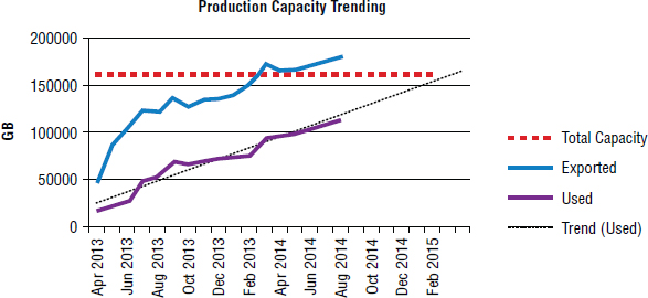
When to Purchase Capacity on Overprovisioned Arrays
You need to establish agreed-upon thresholds with senior management that trigger new capacity purchases, and it is imperative that these are decided with an understanding of your company's purchasing process. For example, if your company takes a long time to approve purchases, and your vendor takes a long time to quote and ship storage, you will not want to run things too close to the bone.
Many companies use at least two trigger points for capacity purchases. Once the first trigger point is reached, a purchase order for more capacity is raised. Some common trigger points include the following:
- Actual available capacity (installed capacity minus used capacity)
- Percentage of available capacity (percentage of installed capacity that is unused)
- Overprovisioning percentage
Based on these triggers, you might implement the following trigger rules:
- As soon as free capacity (installed capacity minus used capacity) reaches less than 10 TB, you kick off the purchasing cycle.
- Once the percentage of available capacity (installed minus used, expressed as a percentage) reaches less than 10 percent, you might kick off the purchasing cycle.
- Once the array becomes more than 60 percent overprovisioned, you might kick off the capacity purchasing cycle.
Each of these rules depends heavily on your environment, and you must understand the growth characteristics of your environment. For example, waiting until an array has only 10 TB of free capacity will be of no use to you if your growth rate on that array is 15 TB per month and it takes you an average of eight weeks to land additional capacity in your environment. In that case, a value of 50 TB or more free capacity might be a better value.
Space Reclamation
Space reclamation is all about keeping thin volumes thin. Thin-provisioning volumes allow you to avoid preallocating capacity up front and allocate only on demand. However, your thin volumes will quickly become bloated if your thin-provisioning array is unable to recognize when the host deletes data. This is where space reclamation comes into play.
Zero Space Reclamation
At a high level, zero space reclamation is the act of recognizing deleted space in a thin volume and releasing that space back to the free pool so that it can be used by other volumes. However, the secret sauce lies in the array being able to know when space is no longer used by a host.
Space Reclamation the Old-School Way
Traditionally, when an OS/hypervisor/filesystem deleted data, it didn't actually delete the data. Instead, it just marked the deleted data as no longer required. That wasn't much use to arrays, as they had no knowledge that this data was deleted, so they were unable to release the extents from the TP volume. In these cases, scripts or tools that would physically write binary zeros to the deleted areas of data were required in order for the array to know that there was capacity that could be released.
Zero space reclamation works on the principle of binary zeros. For an array to reclaim unused space, that space must be zeroed out—the act of writing zeros to the deleted regions.
Host-Integration Space Reclamation
Modern operating systems such as Red Hat Enterprise Linux 6 (RHEL), Windows Server 2012, and vSphere 5 know all about thin provisioning and the importance of keeping thin volumes thin, so they are designed to work smoothly with array-based zero-space-reclamation technologies.
To keep thin volumes thin, these operating systems implement the T10 standards-based UNMAP command that is designed specifically for informing storage arrays of regions that can be reclaimed. The UNMAP command informs the array that certain Logical Block Address (LBA) ranges are no longer in use, and the array can then release them from the TP volume and assign them back to the free pool. There is no more need for scripts and tools to zero out unused space; the OS and filesystem now take care of this for you.
Inline or Post-process Space Reclamation
Some arrays are clever enough to recognize incoming zeros on the fly and dynamically release TP extents as streams of zeros come into the array. Other arrays are not that clever and require an administrator to manually run post-process space-reclamation jobs in order to free up space that has been zeroed out on the host.
Both approaches work, but the inline approach is obviously a lot simpler and better overall, as long as it can be implemented in a way that will not impact array performance.
Overprovisioning Needs Space Reclamation
If your array supports thin provisioning but not space reclamation, you are on a one-way street to a dead end. Yes, you will avoid the up-front capacity wasting of thick volumes. However, your thin volumes will quickly suffer from bloating as data is deleted but not reclaimed by the array. If your array supports thin provisioning and you plan to overprovision, make sure your array also supports space reclamation!
A Space Reclamation Issue to Beware Of
Watch out for potential performance impact in two areas:
- Applications with heavily sequential read patterns
- Performance overhead each time a new page or extent is allocated
If you are overprovisioning, you need to have eagle eyes on capacity usage and trending of your array. If you take your eye off the ball, you could run out of space and be in a world of hurt.
Go into overprovisioning with your eyes wide open. Overprovisioning does not simplify capacity management or storage administration. Anyone who says otherwise probably does not have a lot of hands-on experience with it in the real world.
Pooling and Wide-Striping
Pooling and wide-striping are often used synonymously. Both technologies refer to pooling large numbers of drives together and laying out LUNs and volumes over all the drives in the pool. Figure 3.16 shows three volumes wide-striped over all 128 drives in a pool.
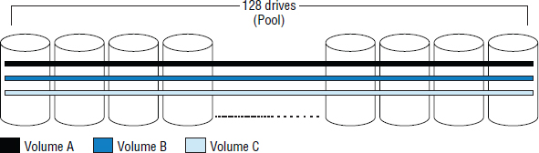
It should be said that arrays that do not implement wide-striping should for the most part be considered dinosaurs. All good arrays support pooling and wide-striping.
Pooling and Performance
Pooling has the ability to improve the performance of volumes on your storage array. This is because all volumes potentially have access to all the IOPS and MB/sec of all of the drives on the backend.
Even if pooling doesn't improve the performance of specific volumes, it will reduce hot and cold spots on the backend, ensuring you get the most performance out of the backend of your array. With pooling, you should not see some drives sitting idle while others are being maxed to their limits.
Pooling and Simplified Management
Aside from maximizing and balancing performance, the dawn of wide-striping has greatly simplified storage design and administration. Back in the day, before we had pooling and wide-striping, storage admins and architects would spend hours making sure that two busy volumes didn't use the same four or eight disks on the array, as this would create hot spots and performance bottlenecks. Excel spreadsheets were pushed to their limits to meticulously track and map how volumes were laid out on the backend. Thankfully, this is now a thing of the past!
These days, you land an array on the ground, create a couple of pools, and start creating volumes. You will still probably want to keep data and log volumes on separate pools, but aside from that, you just create your volumes in a pool and let the array balance them. Hot spots on the backend and spindle-based bottlenecks are now extremely rare.
Make sure your array supports rebalancing when additional drives are added to the backend. The last thing you want is a nicely balanced backend, where all drives are 80 percent used from a capacity and performance perspective, only to install 128 new drives and find that they are 0 percent used in both respects. This would create a horrendous imbalance in the backend as well as a lot of manual work to rebalance things. All good arrays support rebalancing when new drives are admitted to the configuration.
The Future Is in Pools
Pools and wide-striping also tend to be where all the vendors are putting their innovation. For example, things like thin provisioning, deduplication, and space reclamation are all being built on top of pools and do not work well with traditional RAID groups.
Pools and Noisy Neighbors
Some business-critical applications in some organizations demand isolation, and by design, pooling is the exact opposite of isolation.
Tier 1 line-of-business application owners like to feel safe and that they are the center of the world—and in many cases, as far as the business is concerned, these applications are the center of the world. So lumping their beloved applications on the same set of spindles as every other unworthy tier 3 and tier 4 app just isn't going to give them the warm fuzzies. In these cases, many organizations opt to create ring-fenced pools with dedicated drives and other resources, or even deploy these apps on dedicated arrays and servers.
While pools and wide-striping might not be appropriate for every application, they do work for the vast majority. Speaking from several years’ experience in various industry sectors, a rough figure would be that pools are appropriate at least 80 percent to 90 percent of the time. You should rarely, if ever, have to deploy volumes against traditional RAID groups these days. But whatever you do, understand your requirements!
Compression
Compression in the storage industry refers to the process of reducing the size of a data set by finding repeating patterns that can be made smaller. Various complex algorithms can be used to compress data, but the nuts and bolts tend to focus on removing sets of repeating characters and other white space.
Compression of primary storage has never really taken off. Yes, we see it here and there, but the major players have been slow to implement it.
Primary storage is storage that is used for data in active use. Even data that is only infrequently accessed and residing on lower tiers is still considered primary storage. Examples of nonprimary storage include archive and backup storage.
Compression of primary storage has not taken off primarily because of its impact on performance. Nobody wants to wait for their primary storage to decompress data. People moan if recalling a three-year-old email from archive takes more than a few seconds, never mind waiting for a long-running query to a volume that has an additional wait included while the storage array decompresses the data being queried.
That said, compression has its place in the storage world, especially in backup and archive use cases and, somewhat interestingly, in SSD-based storage arrays. There are two common approaches to compression:
- Inline
- Post-process
Let's take a look at both before we move on to consider compression's performance impact and the future of compression.
Inline Compression
Inline compression compresses data in cache memory before it hits the drives on the backend. This can obviously use up lots of cache, and if the array is experiencing high volumes of I/O, the process of compressing data can easily lead to slower response times.
On the positive side, though, inline compression can massively reduce the amount of write I/O to the backend. This has the obvious added benefit that less backend disk space is used, but it also means that less internal bandwidth is consumed. The latter is not always considered, but it can be significant.
Post-process Compression
Post-process compression will first land the uncompressed data on the drives on the backend and then at a later time run a background task to compress the data.
Post-processing data takes away the potential performance impact but does nothing to assist with increasing the available internal bandwidth of the array—which, incidentally, can be a major bonus of compression technology. After all, internal bandwidth is often more scarce and always more expensive than disk capacity.
Whether compression is done inline or post process, decompression will obviously have to be done inline and on demand.
Performance Impact
A major performance problem resulting from data compression can be the time is takes to decompress data. Any time a host issues a read request to an array and that data has to be fetched from the backend, this is a slow operation. If you then add on top of that the requirements to decompress the data, you can be looking at a significantly longer operation. This is never ideal. To mitigate this, many storage arrays use the Lempel-Ziv-Oberhumer (LZO) compression algorithm, which doesn't yield the greatest compression in the world, but is simple and fast.
Compression's Future in Primary Storage
With modern CPUs having cycles to burn, and often compression offloads, compression of primary storage is becoming more feasible. Also the use of flash as a storage medium is helping, as the latency incurred when decompressing data is lower because of the faster read speeds of flash, and the usable capacity gains can make flash a more cost-viable option.
Some storage systems are implementing a combination of inline and post-process techniques, performing inline compression when the array can afford to do so, but when I/O levels increase and the going gets tough, they fall back to post-processing the data.
In NAS devices, you should make sure that compression is done at the block level and not the file level. The last thing you want is to have to decompress an entire file if you need to read only a small portion. In fact, in some instances, such as NAS arrays with spinning disk, you may get increased performance if using a good compression technology.
Two final pieces of advice would be, as always, to try before you buy and test before you deploy. In some use cases, compression will work, and in other use cases it will not. Be careful.
Deduplication
Deduplication differs from compression in that deduplication algorithms look for patterns in a data stream that they have seen before—maybe a long time ago. For example, in the manuscript for this book, the word storage has been used hundreds of times. A simple deduplication algorithm could take a single instance of the word storage and remove every other instance, replacing all other instances with a pointer back to the original instance. If the word storage takes up 4 KB and the pointer takes up only 1 KB, we can see where the savings come from. Obviously, that was an overly simplified example.
Whereas compression eliminates small, repeated patterns that are close together (such as the same 32–128 KB chunk), deduplication eliminates larger duplicates over a wider field of data. Deduplication has had a similar history to compression in that it has been widely adopted for archival and backup purposes but has not seen stellar rates of adoption in primary storage. Again, this is mainly due to the potential performance hit.
Like compression, deduplication should always be done at the block level and never at the file level. In fact, file-level deduplication is probably more accurately termed single instancing. Obviously, block arrays will do only block-based dedupe, but your NAS vendor could attempt to pull the wool over your eyes by selling you file-level single instancing as deduplication. Don't let them do that to you! Deduplication should always be done at the block level, and preferably with a small block size.
Similar to compression, it is generally an inline or a post-process job.
Inline Deduplication
In inline deduplication, data is deduplicated on the front end before being committed to disk on the backend.
Inline dedupe requires hashes and then lookups. Strong hashes consume CPU but give good hit/miss accuracy, whereas weaker hashes consume less CPU but require more bit-for-bit lookups (which is slow on spinning disk but feasible on SSD).
Inline deduplication does not require a bloated landing area but may impact front-end performance.
Post-process Deduplication
Data is written to disk in its bloated form and then later is checked to see whether it already exists elsewhere. If it is determined that the data pattern already exists elsewhere on the array, this instance of the data pattern can be discarded and replaced with a pointer.
A drawback to the post-process method is that you need enough capacity on the backend to land the data in its un-deduplicated form. This space is needed only temporarily, though, until the data is deduplicated. This leads to oversized backends.
The benefit of post-process is that it does not impact the performance on the front end.
What to Watch Out For
On NAS arrays, you need to watch out for file-based single instancing being deceivingly branded as deduplication. As noted earlier, the two are not the same. With file-based single instancing, you need two files to be exact matches before you can dedupe. Two 1 MB Word documents that are identical except for a single character in the entire file will not be able to be deduped. Compare that to block level, which will dedupe the entire file except for the few kilobytes that contain the single-character difference. You always want block dedupe, and the smaller the block size, the better!
The scope of deduplication is also important. Ideally, you want an array that deduplicates globally. This means that when checking for duplicate data patterns, the array will check for duplicate patterns across the entire array. Checking the entire array gives better probability of finding duplicates than confining your search to just a single volume.
Auto-tiering
Sub-LUN auto-tiering is now a mainstay of all good storage arrays. The theory behind auto-tiering is to place data on the appropriate tier of storage based on its usage profile. This usually translates to data that is being accessed a lot—hot data—residing on fast media such as flash, and data that is rarely accessed—cold data—residing on slower media such as large 7.2K Near Line Serial Attached SCSI (NL-SAS) drives.
Sub-LUN
When it comes to auto-tiering, sub-LUN is where the action is. Early implementations of auto-tiering worked with entire volumes. If a volume was accessed a lot, the entire volume was promoted up to higher tiers of storage. If a volume wasn't accessed very often, the entire volume was demoted to the lower tiers of storage. The problem was that parts of a volume could be very hot, whereas the rest could be cold. This could result in situations where a large volume, say 500 GB, was moved into the flash tier when only 10 MB of the volume was being frequently accessed and the remaining 499.99 GB was cold. That is not great use of your expensive flash tier.
Enter sub-LUN technology. Sub-LUN technology divides a volume into smaller extents, and monitors and moves in extents rather than entire volumes. Assuming our 500 GB example volume from earlier, if the extent size was small enough, only the hot 10 MB of the volume would move up to the flash tier, and the remaining cold data could even filter down to lower tiers. That is a much better solution!
The objective is that if, for example, only 20 percent of your data is active with the remaining 80 percent being relatively inactive, you can fit that 20 percent on high-performance drives, and dump the inactive data sets on cheaper, slower drives.
Sub-LUN Extent Size
As always seems the case, when it comes to extent sizes—whether snapshot extents, thin-provisioning extents, or now sub-LUN extents—smaller is better.
The sub-LUN extent size is the granularity to which a volume is broken up for the purposes of monitoring activity and migrating between tiers. A sub-LUN extent size of 7.6 MB means that the smallest amount of data within a volume that can be moved around the tiers is 7.6 MB.
Generally speaking, high-end enterprise-class arrays have smaller extent sizes than midrange arrays, but this is not always true. However, you should find out the extent size used by your array before purchasing it. This information can usually be easily found in the product documentation or by quickly searching the Internet. Some midrange arrays have a sub-LUN extent size of 1 GB, which can be massively wasteful of premium flash-based resources; nobody in their right mind wants to move 1 GB of data into the flash tier if only 50 MB of that extent is actually busy.
Sizing Up Your Tiers
Most arrays and most tiered storage designs are based around three tiers. These tiers are usually as follows:
Tier 1: Flash/SSD
Tier 2: SAS 10K or 15K
Tier 3: NL-SAS 7.2K or 5.4K
How much of each tier to purchase can be highly dependent on your workload, and your vendor or channel partner should have tools available to help you decide.
Generally, the ratios of the three tiers can be represented in a pyramid diagram, as shown in Figure 3.17.
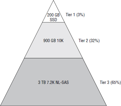
In Figure 3.17, the percentage values indicate the percentage of capacity and not the percentage of drives. While not attempting to suggest the percentages in the diagram should be used in your environment, they are tailored for a mixed workload array in which the workload parameters were not well known at the time of the design, so it may be a good rough starting point for tuning your own configuration.
Monitoring Period
In order to make decisions about which extents to move up and down the available tiers, the array needs to monitor I/O activity on the backend. It can be important that you monitor the backend performance at the right times. For example, if your organization runs its backups overnight, you may want to exclude the backup window from the monitoring schedule so that the backup workloads do not skew the stats and influence the decision-making process. 99 times out of 100, you will not want your backup volumes consuming your higher tiers of storage.
A common approach is to monitor during core business hours on business days, but this may not be appropriate for your environment.
Scheduling Tiering Operations
In addition to deciding when you want to monitor your system, you need to determine data movement windows during which the array is allowed to move extents between the tiers. This, again, will be specific to your business requirements and could be restricted based on how often your array technology allows you to move data. But the point to keep in mind is that moving data about on the backend uses backend resources and, in many cases, cache. Most companies decide to move their data outside business hours. Often this is during the early hours of the morning, such as between 1 a.m. and 4 a.m., though on some systems continuous motion is a better idea.
Exclusions and Policies
Good storage arrays provide you with a means of including and excluding volumes from auto-tiering operations. For example, you might have some volumes that you have determined need to always reside 100 percent in the middle tier.
You may also have volumes that you want to be controlled by the auto-tiering algorithm but you want to restrict the amount of tier 1 space they consume, or you may want to ensure that they are never relegated to the lowest tier.
Your array should allow you to create tiering polices to achieve fine control of your array's auto-tiering behavior if required.
Auto-tiering with Small Arrays
Auto-tiering solutions tend to be better suited for larger configurations and less so for smaller arrays. One of the main reasons is that each tier needs sufficient drives within it to provide enough performance. If the small array also has a large sub-LUN extent size, this will add to the inefficiencies. Also, licensing costs tend not to make auto-tiering solutions as commercially viable in smaller configurations. From a cost, balancing, and performance perspective, the case for using auto-tiering solutions tends to stack up better in larger arrays.
Auto-tiering and Remote Replication
It is easy with some auto-tiering solutions to end up in a situation where your volumes are optimally spread out over the tiers in your source array but not in your target array. This can happen for various reasons, but a major contributing factor is that replication technologies replicate write data only from the source to the target array. Read requests to the source array heavily influence the layout of a volume on the source array. However, the effects of these reads are not reflected on the target array, and hence the replica volume on the target array could well occupy a larger percentage of the lower tiers on the target array. Obviously, if you need to invoke DR, you could see a performance drop due to this.
Storage Virtualization
In this chapter, storage virtualization refers to controller-based virtualization.
Controller-based virtualization is the virtualization of one storage array behind another, as shown in Figure 3.18. In Figure 3.19 later in this section, you can see that write I/Os can be ACKed when they reach the cache in the virtualization controller. Once the data is in the cache of the virtualization controller, it can then be destaged to the virtualized array in a lazy fashion.
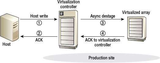
In a storage virtualization setup, one array acts as the master and the other as the slave. We will refer to the master as the virtualization controller and the slave as the virtualized array.
The virtualization controller is where all the intelligence and functionality resides. The virtualized array just provides RAID-protected capacity. None of the other features and functions that are natively available in the virtualized array are used.
A Typical Storage Virtualization Configuration
Configuring a typical storage virtualization requires several steps:
- Configuring the array being virtualized
- Configuring the virtualization controller
- Connecting the virtualization controller and the virtualized array
Let's look at each of these steps more closely, and then you'll see an example of how they all fit together.
Configuring the Array Being Virtualized
Usually the first thing to do is to configure the array being virtualized. On this array, you create normal RAID-protected volumes and present them as SCSI LUNs to the virtualization controller. LUN masking should be used so that only the WWPNs of the virtualization controller have access to the LUNs. These LUNs don't need any special configuration parameters and use normal cache settings. It is important that you configure any host mode options for these LUNs and front-end ports according to the requirements of the virtualization controller. For example, if the virtualization controller imitates a Windows host, you will need to make sure that the LUNs and ports connecting to the virtualization controller are configured accordingly.
It is vital that no other hosts access the LUN that are presented to the virtualization controller. If this happens, the data on those LUNs will be corrupted. The most common storage virtualization configurations have all the storage in the virtualized array presented to the virtualization controller. This way, there is no need for any hosts to connect to the virtualized array.
Configuring the Virtualization Controller
After configuring the array, you configure the virtualization controller. Here you configure two or more front-end ports—yes, front-end ports—into virtualization mode. This is a form of initiator mode that allows the ports to connect to the front-end ports of the array being virtualized and discover and use its LUNs. To keep things simple, the ports on the virtualization controller that connect to the array being virtualized will emulate a standard Windows or Linux host so that the array being virtualized doesn't need to have any special host modes configured.
Connecting the Virtualization Controller and the Virtualized Array
Connectivity is usually FC and can be direct attached or SAN attached. Because of the critical nature of these connections, some people opt for direct attached in order to keep the path between the two arrays as simple and clean as possible.
Once the virtualization controller has discovered and claimed the LUNs presented from the virtualized array, it can pretty much use the discovered capacity the same way it would use capacity from locally installed drives. One common exception is that the virtualization controller usually does not apply RAID to the discovered LUNs. Low-level functions such as RAID are still performed by the virtualized array.
Figure 3.19 shows a virtualized array presenting five LUNs to the virtualization controller. The virtualization controller logs in to the virtualized array, discovers and claims the LUNs, and forms them into a pool. This pool is then used to provide capacity for four newly created volumes that are presented out of the front end of the virtualization controller to two hosts as SCSI LUNs.
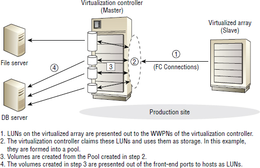
The local storage in the virtualization controller is referred to as internal storage, whereas the storage in the array being virtualized is referred to as external storage or virtualized storage.
Putting It All Together
To understand all the stages of configuring storage virtualization, it is probably best to look at an example of the steps in order. Exercise 3.4 explores this.
EXERCISE 3.4
Configuring Storage Virtualization
The following steps outline a fairly standard process for configuring storage virtualization. The exact procedure in your environment may vary, so be sure to consult your array documentation, and if in doubt consult with your array vendor or channel partner.
On the array being virtualized, perform the following tasks:
- Carve the backend storage into RAID-protected volumes. Usually, large volumes, such as 2 TB, are created.
- Present these LUNs on the front-end ports and LUN-mask them to the WWPNs of the virtualization controller.
- Configure any standard cache settings for these LUNs.
- Configure any host mode settings required by the virtualization controller. For example, if your virtualization controller emulates a Windows host, make sure you configure the host settings appropriately.
On the virtualization controller, perform the following tasks:
- Configure a number of front-end ports as external ports (Virtualization mode). You should configure a minimum of two for redundancy.
Now that the basic tasks have been performed on the virtualization controller and the array has been virtualized, the arrays need to be connected. These connections can be either direct-attached or SAN-attached connections. Once the arrays are connected and can see each other, perform the following steps on the virtualization controller:
- Using the virtualization controller's GUI or Command Line Interface (CLI), discover the LUNs presented on the virtualized array.
- Configure the newly discovered LUNs into a pool.
It can take a while for the LUNs to be discovered and imported on the virtualization controller, and it can take a while for the pool to be created. Once the pool is created, it can usually be used as if it was a nonvirtualized pool using internal disks. From this point, volumes can be created and bound to the new pool. These volumes can be either mapped to hosts on the front end or used to create a pool.
Prolonging the Life of an External Array
One of the potential reasons for virtualizing an array is to prolong its life. Instead of turning the old array off because it's out-of-date and doesn't support the latest advanced features we require, we can plug it into our shiny new array and give it a brain transplant.
This idea works in principle, but the reality tends to be somewhat more complicated. For this reason, even in a difficult economy with diminishing IT budgets, arrays are rarely virtualized to prolong their life.
Some of the complications include the following:
- Having to keep the virtualized array on contractual maintenance congruent to the environment it will continue to serve. It is not the best idea in the world to have the old virtualized array on Next Business Day (NBD) response if it's still serving your tier 1 mission-critical apps.
- Multivendor support can be complicated if you are virtualizing an array from a third-party vendor. This is made all the more challenging when the array you are virtualizing is old, as the vendor is usually not keen for you to keep old kit on long-term maintenance, and the vendor generally stops releasing firmware updates.
Experience has shown that although virtualizing an array to prolong its life works on paper, the reality tends to be somewhat messy.
Adding Functionality to the Virtualized Array
It's common for customers to buy a new tier 1 enterprise-class array along with a new tier 2/3 midrange array and virtualize the midrange array behind the enterprise-class array. This kind of configuration allows the advanced features and intelligence of the tier 1 array to be extended to the capacity provided by the virtualized tier 2 array. Because the array performing the virtualization treats the capacity of the virtualized array the same way it treats internal disk, volumes on the virtualized array can be thin provisioned, deduplicated, replicated, snapshotted, tiered, hypervisor offloaded…you name it.
Storage Virtualization and Auto-tiering
All good storage arrays that support controller-based virtualization will allow the capacity in a virtualized array to be a tier of storage that can be used by its auto-tiering algorithms. If your array supports this, then using the capacity of your virtualized array as your lowest tier of storage can make sound financial and technical sense.
Because the cost of putting disk in a tier 1 array can make your eyes water—even if it's low-tier disk such as 4 TB NL-SAS—there is solid technical merit in using only the internal drive slots of a tier 1 array for high-performance drives. Aside from the cost of loading internal drive slots, they also provide lower latency than connecting to capacity in a virtualized array. So it stacks up both financially and technically to keep the internal slots for high-performance drives.
This leads nicely to a multitier configuration that feels natural, as shown in Figure 3.20.
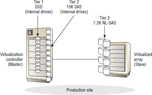
There is no issue having the hot extents of a volume on internal flash storage, the warm extents on internal high performance SAS, but having the coldest and least frequently accessed extents down on external 7.2 K or 5.4 K NL-SAS. This kind of configuration is widely deployed in the real world.
Of course, this all assumes that your virtualization license doesn't cost an arm and a leg and therefore destroy your business case.
Virtualization Gotchas
There is no getting away from it: storage virtualization adds a layer of complexity to your configuration. This is not something that you should run away from, but definitely something you should be aware of before diving in head first.
![]() Real World Scenario
Real World Scenario
Complications That Can Come with Storage Virtualization
A company was happily using storage virtualization until a well-seasoned storage administrator made a simple mistake that caused a whole swath of systems to go offline. The storage administrator was deleting old, unused external volumes—volumes that were mapped from the virtualized array through the virtualization controller. However, the virtualization controller gave volumes hexadecimal numbers, whereas the virtualized array gave volumes decimal numbers. To cut a long story short, the administrator got his hex and decimal numbers mixed up and deleted the wrong volumes. This resulted in a lot of systems losing their volumes and a long night of hard work for several people. This complexity of hex and decimal numbering schemes would not have existed in the environment if storage virtualization was not in use.
Depending on how your array implements storage virtualization, and also sometimes depending on how you configure it, you may be taking your estate down a one-way street that is hard to back out of. Beware of locking yourself into a design that is complicated to unpick if you decide at a later date that storage virtualization is not for you.
If your array is not designed and sized properly, performance can be a problem. For example, if you don't have enough cache in your virtualization controller to deal with the capacity on the backend, including capacity in any virtualized arrays, you may be setting yourself up for a bunch of performance problems followed by a costly upgrade. Also, if the array you are virtualizing doesn't have enough performance—usually not enough drives—to be able to destage from cache quickly enough, you can make the cache of your virtualization head a choking point.
While on the topic of performance, by far the most common implementation of storage virtualization these days is using the virtualized array for cheap and deep tier 3 storage. It is rare to see customers loading virtualized arrays up with high-performance drives.
Finally, cost can be an issue if you don't know what you're getting yourself into. Virtualization licenses rarely come for free.
Hardware Offloads
Hardware offloads, sometimes referred to as hardware accelerations, are a relatively recent trend in the open systems storage world. A hardware offload is the act of executing a function in dedicated hardware rather than software. In respect to storage, this usually translates into operating systems and hypervisors offloading storage-related functions such as large copy jobs and zeroing out to the storage array.
There are a few objectives in mind when implementing hardware offloads to a storage array. These tend to be as follows:
- Improve performance
- Reduce the load on the host CPU
- Reduce the load on the network
While it's true that most servers these days have CPU cycles to burn, many storage-related tasks can still be performed faster and more efficiently by offloading them to the storage array.
Let's look at a few of the more popular examples in the real world.
VMware VAAI
VMware was perhaps the first vendor in the open systems world to push the notion of hardware offloads. VMware's vStorage API for Array Integration (VAAI) is a suite of technologies designed to offload storage-related operations to a VAAI-aware storage array. There are VAAI offloads for both block storage and NAS storage, referred to as block primitives and NAS primitives, respectively.
Block storage primitives are based on T10 SCSI standards and are natively supported by any storage array that supports those T10 standards, although be sure to check the VMware Hardware Compatibility List (HCL) before making any assumptions. VAAI for NAS, on the other hand, requires a plug-in from your NAS vendor.
Despite the name—vStorage API for Array Integration—VAAI primitives are not really APIs. Instead the vSphere hypervisor is simply written to understand SCSI standards and SCSI commands that allow it to offload storage-related functions to a storage array that supports the same SCSI commands.
Let's look at each of the available VAAI offloads.
ATS
If you know anything about Virtual Machine File System (VMFS), you will know that certain metadata updates require a lock to ensure the integrity of the updated metadata and the entire VMFS volume.
Back in the day, the only locking mechanism that was available was a SCSI reservation. And the problem with a SCSI reservation is that it locks an entire LUN, meaning that any time you made a metadata update you had to lock the entire LUN. And when a LUN is locked, it cannot be updated by any host other than the host that issued the reserve command. That is not the end of the world if we're talking about small, lightly used VMFS volumes. However, this could become a problem with large, heavily used VMFS volumes accessed by multiple hosts. This is where atomic test and set (ATS) comes to the rescue!
ATS, also known as hardware-assisted locking, brings two things to the party:
Extent-Based Locking Extent-based locking means that you no longer have to lock up the entire LUN with a SCSI reserve when updating the metadata in a VMFS volume. You need to lock only the extents that contain the metadata being updated.
More-Efficient Locking Procedure The act of engaging and releasing the extent-based lock is offloaded to the storage array, and the locking mechanism requires fewer steps, making it quicker and more efficient.
Both of these added significantly to the scalability of VMFS and were major factors behind the ability to deploy larger VMFS datastores.
Since the initial release of VAAI, ATS has now been formalized as a T10 SCSI standard using SCSI opcode 0x89 and the COMPARE_AND_WRITE command. This ensures standards-based implementations by all supporting storage arrays.
Hardware-Accelerated Zeroing
Certain situations in VMware environments require the zeroing out of entire volumes. For example, eager zeroed thick (EZT) volumes are volumes that are wiped clean by writing zeros to every sector in the volume. This has positive security implications by ensuring that no data from a volume's previous life can inadvertently be visible. It also has potentially positive performance implications by not requiring ESX to have to zero a block the first time it writes to it—although don't expect the performance improvements to blow you away.
Let's look at a quick example of hardware-accelerated zeroing in action. Assume a volume with 1,000 blocks and that you need to zero out this entire volume. Without hardware-accelerated zeroing, ESX would have to issue the set of commands outlined in Figure 3.21.
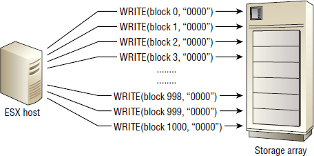
With the introduction of hardware-accelerated zeroing, the exact same outcome can be achieved via a single command, as shown in Figure 3.22.
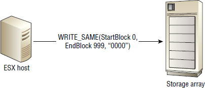
Not only does this offload the operation from the ESX host, freeing up CPU cycles, it also vastly reduces network chatter, as the ESX host can issue a single command and the array can give a single response. In addition, the storage is probably able to do the work faster. The net result is that the operation completes faster and uses less ESX CPU and less network resources.
Hardware-accelerated zeroing works via the T10 SCSI standard WRITE_SAME command (opcode 0x93).
Hardware-Accelerated Copy
Popular VMware-related operations, such as Storage vMotion and creating new VMs from a template, utilize large data-copy operations. Hardware-accelerated copy uses the SCSI EXTENDED_COPY command (opcode 0x83) to offload the heavy lifting work of the data copy to the storage array. Figure 3.23 shows a large copy operation without and with the use of EXTENDED_COPY.
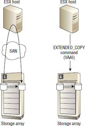
In Figure 3.23, the operation on the left that does not use the EXTENDED_COPY offload requires all data being copied from the source volume to the target volume to pass up from the array, through the SAN, through the HBAs in the ESX host, through the kernel data mover engine, back out through the HBA, back down through the SAN, and back to the storage array. In contrast, the operation on the right shows a single EXTENDED_COPY command issued from the ESX host to the array. The array then copies the data internally without it having to pass all the way up the stack, through the host, and back down again.
With the use of the EXTENDED_COPY hardware assist, network bandwidth utilization can be dramatically decreased, as can host-based resource utilization.
Thin Provisioning Stun
Thin provisioning stun (TP Stun) is an attempt to gracefully deal with out-of-space conditions on overprovisioned storage arrays. TP stun is a mechanism by which virtual machines that request additional space from a storage array that has run out space can be paused rather than crash. This is achievable because the storage array can now inform the host that its disk is full rather than just issuing a write fail to the host, allowing the host to more gracefully deal with the scenario. Once the array has more space, the condition is cleared and VM can be resumed.
While this might not sound perfect, it's an attempt to make the most of what is a nightmare scenario. This is of course relevant only on thin-provisioning storage arrays that are overprovisioned and VMs that reside on datastores that are thinly provisioned from the storage array.
VAAI and Zero Space Reclamation
The latest versions of VMware are now fully aware of array-based thin provisioning and optimized assist in the ongoing effort to keep thin volumes thin.
VAAI now utilizes the T10 SCSI standard UNMAP command to inform the storage array that certain blocks are no longer in use. Examples include deleted VMs or VMs that have been migrated to other datastores.
Full File Clone for NAS
Full file clone for NAS brings offloading the cloning of virtual disks to the VMware NAS party. This feature is similar to the functionality of EXTENDED_COPY in the block world, in that it offloads VM copy operations to the NAS array. However, it is not quite as functional as its block counterpart, as it can be used for only clone operations and cannot be used for Storage vMotion (meaning that the VM must be powered off). Storage vMotion operations still revert to using the VMkernel's software data mover.
Fast File Clone for NAS
Fast file clone for NAS brings support for offloading VM snapshot creation and management to the native snapshot capabilities of the NAS array. This enables snapshots to be created much quicker and with less network-related traffic.
No ATS Needed for NAS
Interestingly, there is no need for the equivalent of an ATS primitive in the NAS world, as the NAS world has never been plagued with rudimentary locking systems such as the SCSI RESERVE mechanism. This is because NAS arrays understand and own the underlying exported filesystem and therefore have native advanced file-level locking capabilities.
Microsoft ODX
With Windows 8 and Server 2012, Microsoft introduced Offloaded Data Transfer (ODX) to the world. ODX is a data-copy offload technology, designed to offload data-copy functions to intelligent storage arrays in much the same way that VMware does with VAAI. It could be said that ODX is to Windows what VAAI is to VMware. The difference is that VMware has been doing it for longer, and therefore has more capabilities and more maturity, though this will no doubt level out over time.
As ODX is similar to some VAAI primitives, it exists to speed up certain storage-based operations such as large copy operations and bulk zeroing, while at the same time saving on host CPU, NIC utilization, and network bandwidth.
ODX for Large File Copies
Figure 3.24 shows how ODX works for a large copy operation.
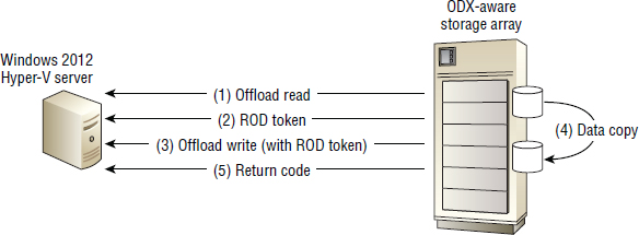
In the large copy operation represented in Figure 3.24, the host running Windows Server 2012, or later, issues an offload read command to the ODX-aware array. The array responds with a 512-byte token that is an array-specific logical representation of the date to be copied. This token is known as a representation of data (ROD) token. The host then issues an offload write request, with the associated ROD token, to the array. The array then performs the copy without the data ever leaving the array.
ODX can also work between two arrays that both support this particular ODX configuration.
ODX works with the following technologies:
- Hyper-V virtual hard disks (VHD)
- SMB shares (sometimes referred to as CIFS)
- Physical disks
- FC, iSCSI, FCoE, SAS
ODX will be invoked to perform the data copy any time a copy command is issued from the CLI, PowerShell prompt, Windows Explorer, or Hyper-V migration job, as long as the server is running Windows Server 2012 or later and the underlying storage array supports ODX. However, things like deduplication and Windows BitLocker-encrypted drives do not work with the initial release of ODX. Future versions of these filter drivers will potentially be ODX aware.
ODX utilizes T10 XCOPY LITE primitives, making it standards based.
As with all developing technologies, it is spreading its wings. Check with vendors and Microsoft for supported configurations. Things to beware of include Resilient File System (ReFS), dynamic disks, and similar developments.
ODX and Bulk Zeroing
ODX can also be used to perform bulk zeroing by using the Well Known Zero Token ROD token.
A ROD token can be a vendor-specific 512-byte string that, for example, represents the data range to be copied. Alternatively, a ROD token can be a Well Known token such as the Zero Token that is used to perform bulk zero operations.
Chapter Essentials
Dual Controller and Grid Architectures Dual-controller architectures, sometimes referred to as midrange, provide many of the advanced features seen in enterprise-class grid architectures but at a cheaper price point. Dual-controller architectures are also limited in scalability and do not deal with hardware failures as well as grid architectures. Grid architectures offer scale-out and deal better with hardware failures, but at a higher cost.
Redundancy Redundancy is a hallmark of storage designs. Most storage arrays employ redundancy at every level possible, ensuring that failed components do not interrupt the operation of the array. Even at the host level, multiple paths are usually configured between the host and storage in multipath I/O (MPIO) configurations, ensuring that the loss of a path or network link between the host and storage array does not take the system down.
Replication Array-based replication makes remote copies of production volumes that can play a vital role in disaster recovery (DR) and business continuity (BC) planning. Depending on your application and business requirements, remote replicas can either be zero-loss bang-up-to-date synchronous replicas or they can lag slightly behind, using asynchronous replication technology. Asynchronous replication technologies can have thousands of miles between the source and target volumes, but synchronous replication requires the source and target to be no more than ∼100 miles apart.
Thin Provisioning Thin-provisioning technologies can be used to more effectively utilize the capacity in your storage arrays. However, if overprovisioning an array, you must take great care to ensure that your array does not run out of available space.
Sub-LUN Tiering Sub-LUN tiering technologies allow you to place data on the most appropriate tier of storage—frequently accessed data on fast media, and inactive data on slow media. This can improve the performance of your array and bring costs down by not having to fill your array with fast disks when most of your data is relatively infrequently accessed.
Summary
In this chapter we covered all things storage array related. We discussed; architectural principles, including the front-end, the backend, the importance of cache, different types of persistent media, and LUNs and volumes. We even touched on snapshots and clones, as well as replication technologies, though these will be covered in more detail in their own dedicated chapters of this book. We talked about pros and cons, use cases, and impact and disruptive nature of flash-based solid state media.
We also talked about some of the advanced features, and so-called intelligence, of storage arrays, including tiering, deduplication, and hardware offloads, many of which integrate with server- and hypervisor-based technologies.