Chapter
5

Fibre Channel SAN

TOPICS COVERED IN THIS CHAPTER:

• What a Fibre Channel SAN is
• HBAs and CNAs
• Switches and directors
• Cabling
• Fabric services
• Zoning
• SAN topologies
• FC routing and virtual fabrics
• Flow control
• Troubleshooting

This chapter gets under the hood with the important technologies that make up a Fibre Channel SAN. It covers the theory and the practical applications, and shares tips that will help you in the real world. You'll learn the basics about redundancy; cabling; switch, port, and HBA configuration; as well as more-advanced topics such as inter-switch links, virtual fabrics, and inter-VSAN routing.

By the end of the chapter, you will know all the necessary theory to deploy highly available and highly performing FC SANs, as well as a few of the common pitfalls to avoid. You'll also have the knowledge required to pass the FC SAN components of the exam.

What Is an FC SAN?

First up, let's get the lingo right. FC SAN is an abbreviation for Fibre Channel storage area network. Most people shorten it to SAN.

At the very highest level, an FC SAN is a storage networking technology that allows block storage resources to be shared over a dedicated high-speed Fibre Channel (FC) network. In a little more detail, Fibre Channel Protocol (FCP) is a mapping of the SCSI protocol over Fibre Channel networks. So in effect, SCSI commands and data blocks are wrapped up in FC frames and delivered over an FC network. There is plenty more to come about that in this chapter.

Because FCP encapsulates SCSI, it is technically possible to share any SCSI device over an FC SAN. However, 99.9 percent of devices shared on an FC SAN are disk storage devices, or tape drives and tape libraries.

Devices shared on an FC SAN, like all SCSI devices, are block devices. Block devices are effectively raw devices that for all intents and purposes appear to the host operating system and hypervisor as though they are locally attached devices. Also they do not have any higher levels of abstraction, such as filesystems, applied to them. That means that in an FC SAN environment, the addition of filesystems is the responsibility of the host accessing the block storage device.

Figure 5.1 shows a simple FC SAN.

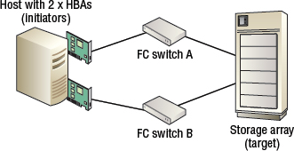
As shown in Figure 5.1, the following are some of the major components in an FC SAN:

• Initiators (commonly referred to simply as hosts or servers)
• Targets (disk arrays or tape libraries)
• FC switches

Initiators and targets in Figure 5.1 are SCSI concepts that can be thought of as clients and servers as in the client-server networking model. Initiators are synonymous with clients, whereas targets are synonymous with servers. More often than not, initiators issue read and write commands to targets over the FC SAN.

Initiators are usually hosts, or to be more accurate, they are HBA or CNA ports in a host. Targets are usually HBA or CNA ports in a storage array or tape library. And the SAN is one or more FC switches providing connectivity between the initiators and targets. Simple.

Why FC SAN?

The traditional approach of deploying direct-attached storage (DAS) inside servers has pros and cons. Some of the pros are that DAS storage is accessed over very short, dedicated, low-latency, contention-free interconnects (SCSI bus). This guarantees quick and reliable access to devices. However, some of the cons of DAS include increased management, low utilization capacity islands, and limited number of devices such as disk drives.

The idea behind FC SAN technology was to keep the pros but overcome the cons of DAS storage. As such, SAN technology provides a high-speed, low-latency storage network (a channel) that is relatively contention free—especially when compared with traditional Ethernet networks. SANs also get rid of capacity islands by allowing large numbers of drives to be pooled and shared between multiple hosts. They also simplify management by reducing the number of management points. While FC SANs come at a cost ($), they have served the data center well for quite a number of years. However, they are under threat.

The emergence of several new and important technologies is threatening the supremacy of the SAN in corporate IT. Some of these technologies include the following:

• Data center bridging (DCB) Ethernet—sometimes referred to as converged enhanced Ethernet (CEE)
• Cloud technologies
• Locally attached flash storage

Cloud storage and cloud everything is squeezing its way into many IT environments, usually starting at the bottom but working its way to the top. Common examples include test and development environments moving to the cloud, often leading to staging and some production requirements eventually ending up in the cloud. At the top, business-critical line-of business applications—which are more immune to the cloud because of their high-performance, low-latency requirements—are benefitting from locally attached flash storage—where flash is placed on the server's PCIe bus, putting it close to the host CPU and memory. That just leaves the rest of the production environment that is too important to be trusted to the cloud but doesn't require ultra-low latency. But even this use case is under pressure from FCoE, which maps FCP over 10 GB DCB Ethernet. All in all, the FC SAN is under extreme pressure, and it should be! But it isn't about to go away overnight or without a fight. A good set of FC skills will serve you well in FCoE environments in the future.

Next let's take a look at some of the major technology components that make up an FC SAN.

FC SAN Components

FC SANs are made up of several key components—some physical, some logical. In this section, you'll consider the following, and more, in greater detail:

• Host bus adapters and converged network adapters
• FC switches and directors
• FC storage arrays
• FC cabling
• FC fabrics
• FC simple name server
• Zoning
• FC addressing
• FC classes of service
• VSAN technology

Physical Components

At a very high level, a SAN comprises end devices and switches. The end devices communicate via the switches.

We usually think of end devices—sometimes called node ports, or N_Ports—as servers and storage arrays. However, to be technically accurate, end devices are ports on HBAs and CNAs installed in servers, storage arrays, and tape devices. End devices connect to switches via cables. Sadly, data center networking technologies have not made the leap to wireless. FC SANs use optical fiber cables. Multiple switches can be linked together to form larger fabrics.

Anyway, those are the basics. Let's take a closer look at each of the FC SAN components.

HBAs and CNAs

Hosts and servers connect to the SAN via one or more Fibre Channel host bus adapters (HBAs) or converged network adapters (CNAs) that are installed on the PCIe bus of the host. In SCSI parlance, these are the initiators on the SAN.

As mentioned earlier, HBAs and CNAs can be implemented either as PCIe expansion cards or directly on the motherboard of a server—a la LAN on motherboard (LOM).

Each HBA and CNA has its own dedicated hardware resources that it uses to offload all FCP-related overhead from the host CPU and memory. This offloading is a key reason that FC SAN is a fast, low-overhead, but relatively expensive, storage networking technology.

Also, most HBAs and CNAs come with a BIOS, meaning that the servers they are installed in can boot from SAN.

As far as hypervisors and operating systems are concerned, HBAs and CNAs show up on the PCI device tree as SCSI adapters that provide access to standard raw SCSI devices known as LUNs. The OS and hypervisor are unaware that the storage devices they are accessing are over a shared network.

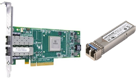
HBAs and CNAs often support either copper direct-attach cables (DACs) or optical transceivers. When you buy the HBA or CNA, you typically have to specify which of the two you want. Generally speaking, optical costs more but supports longer distances, requires less power, and is more popular. These transceivers are often either SFP or SFP+ modules. SFP stands for small form-factor pluggable, and SFP+ is an enhanced version of SFP that supports higher data rates, including 10 GB Ethernet. Both types of transceiver are hot-pluggable. Figure 5.2 shows an HBA with optical transceivers as well as an SFP optic.

FC Switches and Directors

FC switches and FC directors are essentially the same thing—physical network switches that contain multiple physical ports and that support the FC Protocol.

Switches and directors provide connectivity between end devices such as hosts and storage. They operate at layers FC-0, FC-1, and FC-2 and provide full bandwidth between communicating end devices. In addition, they provide various fabric services that simplify management and enable scalability. Also, if multiple FC switches are properly networked together, they merge and form a single common fabric.

The difference between directors and switches is by convention only, so don't get hung up on it! Convention states that larger switches, usually with 128 or more ports, are referred to as directors, whereas those with lower port counts are referred to as merely switches, departmental switches, or workgroup switches. To be honest, most people these days just use the term switch.

That said, directors have more high-availability (HA) features and more built-in redundancy than smaller workgroup-type switches. For example, director switches have two control processor cards running in active/passive mode. In the event that the active control processor fails, the standby assumes control and service is maintained. This redundant control processor model also allows for nondisruptive firmware updates. Smaller workgroup switches do not have this level of redundancy.

Directors tend to be blade-based architectures that allow you to pick and choose which blade types to populate the director chassis with. These blades come in varying port counts (such as 48-port or 64-port) as well as offering different services (such as 16 Gbps FC switching, 10 GB FCoE-capable DCB Ethernet networking, encryption capabilities, and so on).

Before you start making any changes regarding your blades, you need to determine which slots in a director switch are populated, as well as what kind of blades each slot is populated with. Exercise 5.1 shows how you can easily do this.

Switch Ports

FC switches and directors contain multiple ports of varying types. At a physical level, these port types will be either optical or copper SFP/SFP+ ports supporting either FCP or DCB Ethernet/FCoE. Optical is far more popular than copper, but we'll discuss this in more detail soon. As mentioned when we discussed HBAs and CNAs, SFP is an industry-standard pluggable connector.

The following sfpshow command on a Brocade switch shows detailed information about SFP modules installed in the switch:

LegendarySw01:admin> sfpshow
Slot 1/Port 0: id (sw) Vendor: HP-A BROCADE
Serial No: UAA110130000672U Speed: 2,4,8 MB/s

From this, you can see that this SFP is seated in port 0 in slot 1. You can also see that it has a shortwave (sw) laser, you can see its serial number, and you can see that it supports transmission speeds of 2, 4, and 8 MB/s.

Switch ports also have logical parameters. In an FC SAN, a switch port can be in any one of many modes. The most important and most common of these modes are explained here:

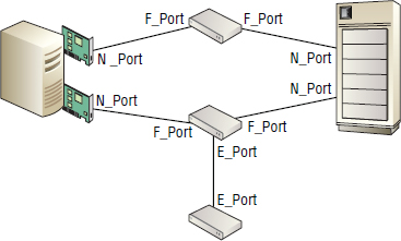
U_Port This is the state that FC ports are typically in when unconfigured and uninitialized.

N_Port This is the node port. End devices in a fabric such as ports in server or storage array HBAs log in to the fabric as N_Ports. Host N_Ports connect to switch F_Ports.

F_Port Switch ports that accept connections from N_Ports operate as fabric ports.

E_Port The expansion port is used to connect one FC switch to another FC switch in a fabric. The link between the two switches is called an ISL.

EX_Port This is a special version of the E_Port used for FC routing. The major difference between E_Ports and EX_Ports is that E_Ports allow the two switches to merge fabrics, whereas EX_Ports prevent fabrics from merging.

There are other port modes, but those listed are the most common.

Figure 5.3 shows N_Port, F_Port, and E_Port connectivity.

Port Speed

As you saw earlier in the output of the sfpshow command, switch ports can operate at different speeds. Common FC speeds include the following:

• 2 Gbps
• 4 Gbps
• 8 Gbps
• 16 Gbps

FCoE/DCB Ethernet ports commonly operate at the following:

• 10 GB
• 40 GB

FC ports—HBA ports, switch ports, and storage array ports—can be configured to autonegotiate their speed. Autonegotiate is a mini-protocol that allows two devices to agree on a common speed for the link. More often than not, this works, with the highest possible speed being negotiated. However, it does not always work, and it is good practice in the real world to hard-code switch-port speed at both ends of the link. For example, if a host HBA that supports a maximum port speed of 8 Gbps is connected to a switch port that supports up to 16 Gbps, you would manually hard-code both ports to operate at 8 Gbps. This practice may be different for FCoE switches and blades that have DCB ports running at 10 GB or higher. For FCoE use cases, consult your switch vendor's best practices.

Domain IDs

Every FC switch needs a domain ID. This domain ID is a numeric string that is used to uniquely identify the switch in the fabric. Domain IDs can be administratively set or dynamically assigned by the principal switch in a fabric during a reconfigure fabric event. The important thing is that a domain ID must be unique within the fabric. Bad things can happen if you configure two switches in the same fabric with the same domain ID.

Principal Switches

Each fabric has one, and only one, principal switch. The principal switch is the daddy when it comes to the pecking order within a fabric. What the principal switch says, goes!

Principal switches are responsible for several things in a fabric, but the things that will be most pertinent to your day job are the following:

• They manage the distribution of domain IDs within the fabric.
• They are the authoritative source of time in a fabric.

Aside from these factors, you shouldn't have to concern yourself with the role of the principal switch in your day job.

Native Mode and Interoperability Mode

FC fabrics can operate in either native mode or interoperability mode. Your switches will be operating in native mode 99.9 percent of the time, and this is absolutely the mode you want them operating in.

Interop modes were designed to allow for heterogeneous fabrics—fabrics containing switches from multiple vendors. In order to allow for these heterogeneous configurations, interop modes disable some advanced and vendor-specific features. Use cases for interop mode tend to be restricted to situations such as acquisitions, where two companies’ IT environments come together and have fabrics running switches from different vendors. But even in those circumstances, merging such fabrics and running in interop mode is rarely a good experience. The best advice to give on interop modes is to avoid them at all costs!

However, if you do need to operate fabrics with switches from different vendors, there is now a much better way than using interop modes. A new technology known as NPV has come to the rescue, and we'll talk about it later in the chapter.

So, with what you have learned so far, the following switchshow command on LegendarySw01 tells us a lot of useful information:

LegendarySw01:admin> switchshow
SwitchNAme:   LegendarySw01
SwitchType:   62.3
SwitchState:  Online
SwitchMode:   Native
SwitchRole:   Principal
SwitchDomain: 44
SwitchId:     fffXXX
SwitchWwn:    10:00:00:05:AA:BB:CC:DD
Zoning:       ON (Prd_Even1)
SwitchBeacon: OFF


Index Port Address Media Speed State     Proto
==============================================
  0   0    220000  cu    8G    Online    FC  F_Port 50:01:43:80:be:b4:08:62
  1   1    220100  cu    8G    Online    FC  F_Port 50:01:43:80:05:6c:22:ae

FC Hubs

As with the rest of the networking world, FC hubs have been superseded by switches, and that is good. Switches are far more scalable and performant than hubs.

Technically speaking, FC hubs operated at the FC-0 layer and were used to connect FC-AL (arbitrated loop) devices. Due to FC-AL addressing limitations, hubs could address only 127 devices, but in practice were even smaller. FC-AL hubs also required all devices to share bandwidth and arbitrate for control of the wire, ensuring that only a single device could communicate on the hub at any one point in time.

Switches, on the other hand, operate up to the FC-2 layer, provide massive scalability, allow multiple simultaneous communications, and provide full nonblocking bandwidth to all connected devices.

Thankfully, FC hubs are generally a thing of the past, and you are unlikely to see them anywhere other than a computer history museum.

FC Storage Arrays

As this book contains an entire chapter dedicated to storage arrays, this section touches on them only lightly.

In an FC SAN, a storage array is an end point/end device with one or more node ports (N_Ports). These node ports are configured in Target mode—and therefore act as SCSI targets—accepting SCSI commands from SCSI initiators such as server-based HBAs and CNAs. Because they are node ports, they participate fully in FC SAN services, such as registering with and querying the name server and abiding by zoning rules.

Storage arrays tend to house lots (hundreds or even thousands) of disk and flash drives that are shared over the FC SAN as block devices referred to as either LUNs or volumes.

Cables

Don't overlook cabling, as it is a critical component of any SAN. Sadly, FC hasn't made the jump to wireless. Nor have any other major data-center networking technologies, for that matter. Therefore, cables and cabling are pretty damn important in SAN environments. Let's kick off with a few basics and then get deeper.

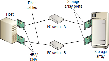
Almost all FC SAN cabling is optical fiber. Optical fiber transmits data in the form of light that is generated by lasers or LEDs. Copper cabling can be used, but this is rare compared to optical. Optical may be used in Top of Rack (ToR) or End of Row (EoR) situations. Some storage vendors used copper cabling on their old FC backends before moving to SAS backends. All optical fiber cabling consists of two pairs of fibers—transmit (TX) and receive (RX)—allowing for full-duplex mode.

Figure 5.4 shows a simple FC SAN with two end devices and an FC switch, and points out the location of some physical components.

Right then, let's get into some detail. Optical fiber cables come in two major flavors:

• Multi-mode fiber (MMF)
• Single-mode fiber (SMF)

Multi-mode fiber transmits light from shortwave lasers, whereas single-mode fiber transmits light from a longwave laser.

When it comes to SAN cabling, multi-mode fiber is the undisputed king of the data center. This is thanks to two things:

• Multi-mode fiber is cheaper than single-mode.
• Multi-mode fiber can easily transmit data over the kinds of distances common to even the largest of data centers.

Single-mode fibers and their associated longwave lasers (optics) are more expensive and tend to be used by telecommunications companies that require longer cable runs, such as hundreds of miles.

All fiber cables—multi-mode and single-mode—are made up of the following major components:

• Core
• Cladding
• Jacket

The core is the insanely small glass or plastic cylinder at the center of the cable that carries the light. If you have seen a stripped fiber cable and think you have seen the core of the cable with your naked eye, you are either Superman or you saw something that wasn't the core. The core of a fiber cable is far too small to be seen by the naked eye!

Surrounding the core is the cladding. The cladding protects the core and ensures that light does not escape from the core.

The outer sheath of all fiber cables is referred to as the jacket. Jackets are usually color coded according to the type of fiber they carry.

Yes, there are other layers and substances between the cladding and the jacket. However, knowledge of them is of no value to you in your day-to-day job.

Figure 5.5 shows the core, cladding, and jacket of a fiber-optic cable.

Multi-Mode Fiber

Multi-mode fiber has a relatively large core diameter compared to the wavelength of the light that it carries, allowing the electronics and lasers that generate the light to be less precise, and therefore cheaper, than those used with single-mode fiber.

As light is injected onto a multi-mode fiber, it can enter the cable at slightly different angles, resulting in the light waves bouncing off the core/cladding perimeter as it travels the length of the cable. This is shown in Figure 5.6.

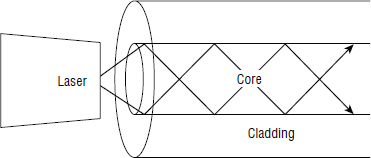
However, over distance, these discrete light beams crisscross, resulting in some signal loss referred to as attenuation. The longer the cable is, the more crisscrossing of light beams occurs, resulting in increased attenuation. Multi-mode fiber can't do very long distances.

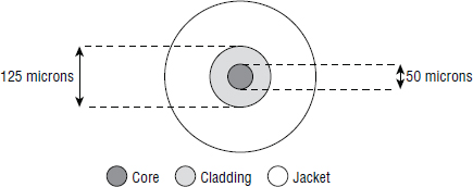
Multi-mode fiber comes in the following two core/cladding options:

• 62.5/125 μm
• 50/125 μm

More often than not, these are referred to as 62.5 micron and 50 micron, respectively. 62.5 and 50 refer to the cross-sectional size of the core in microns. A 50 μm core allows light to be sent more efficiently than 62.5, so it is now more popular than 62.5.

The relatively large core size of multi-mode cables—obviously incredibly small, but large compared to single-mode—means that they can be manufactured to a slightly lower-quality, less-precise design than single-mode cables. This makes them cheaper than single-mode.

Multi-mode fibers are also categorized by an optical multi-mode (OM) designator:

• OM1 (62.5/125)
• OM2 (50/125)
• OM3 (50/125) sometimes referred to as laser optimized
• OM4 (50/125)

By convention, the OM1 and OM2 jacket color should be orange, whereas the OM3 and OM4 jacket color should be aqua (light blue). However, most fiber cables can be purchased in just about any color you wish, and some people choose color schemes that make managing their data center easier. One example is having one cable color for one fabric and another cable color for the other fabric. This will stop you from mixing up your cabling between fabrics. However, a better option might be color-coding the cable connectors rather than the actual cable jackets.

Typically, each time the speed of FCP is increased, such as from 4 Gbps to 8 Gbps, or from 8 Gbps to 16 Gbps, the maximum transmission distance for a given cable type drops off. Table 5.1 shows the maximum distances supported by different multi-mode cable types at the various common FCP speeds.

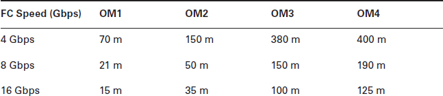
Table 5.1 should help you know which cable type you need to buy. While some companies are now opting for OM3 everywhere, doing this will see you paying more money unnecessarily if you are running cables within a rack or between adjacent racks. On the other hand, using OM3 everywhere for structured cable runs might be a good idea as this future-proofs your infrastructure for things like 40 GB and 100 GB Ethernet. However, intra-cabinet and adjacent cabinet runs do not yet require OM3, and if at some point in the future they do, they can be easily ripped and replaced.

Single-Mode Fiber

Single-mode fiber cables carry only a single beam of light, typically generated by a longwave laser. Single-mode fiber cables are narrow, relative to the wavelength of the laser, meaning that only one mode is captured and therefore there isn't the interference or the excessive reflecting off the core/cladding boundary while light travels the length of the cable. This results in single-mode fiber being able to carry light over distances measured in miles rather than feet. Single-mode fiber cables also tend to be more expensive than multi-mode.

Single-mode fiber core size is usually 9 μm but still with a 125 μm cladding. This 9 μm core requires extremely precise engineering and is a major reason for single-mode fiber being more expensive than multi-mode.

Single-mode fiber is less popular in data centers than multi-mode, and commonly has a yellow jacket.

Bend Radius and Dust

Because fiber cables have a glass core, you need to be really careful when bending them.
Bend them too far, and you will break them. And they're not cheap, so you've been warned!

When talking about bending fiber cables, we use the term bend radius. The minimum bend radius is as tight as a cable can be bent without seriously damaging it.

If you bend the cable too tightly, you can often leave a visible kink in the cable, making it easy to see a broken cable. However, even if you don't kink the cable or crack the glass core, you can stress the cladding so much that it loses its refractive capability—its ability to keep light within the core. Either way, the cable is damaged and will only give you a headache if you continue to use it.

The recommended minimum bend radius for a fiber cable varies depending on the type of fiber cable—OM1 differs from OM3, single-mode differs from multi-mode, and so on. As a general rule, the larger then bend radius the better, a general rule of no less than 3 inches would be a good place to start. That way, you reduce the risk of damage from bending. Make sure you always adhere to the manufacturer's recommendation and don't take risks!

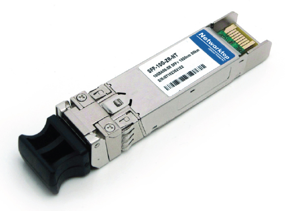
We should also point out that dust on the end of a cable connector or on an optical switch port can cause issues such as flaky connections or connections that log high error counts. This is why new fiber cables come with a rubber or plastic cap—to keep dust out. Not enough people follow the good practice of properly cleaning the tips of fiber cables before using them. Keep your cable ends clean! Figure 5.7 shows an SFP optic with a rubber dust cover.

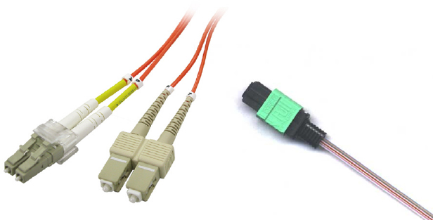
Cable Connectors

Most fiber cables come with male connectors that allow them to be easily popped into and out of switch, HBA, and storage array ports—a process sometimes called mating. While lots of fiber connector types are available, there are a few that you will need to be familiar with as storage administrator, so we'll take a look at these.

SC and LC are probably the most common connectors. SC stands for standard connector, and LC stands for lucent connector. Both are male connectors. LC connectors are only half the size of SC connectors, and for this reason are becoming more and more popular. Half the size can equal double the density.

Another commonly used cable is the MPO or MTP cable. MTP, which stands for multi-fiber termination push-on, is a ribbon cable that carries multiple fibers (usually 12 or 24) and terminates them at a single connector. MTP is a variation of the MPO connector.

Other connector types do exist, but SC, LC, and MTP are by far the most popular in most modern data centers.

Figure 5.8 shows SC, LC, and MTP cable connectors.

If fiber cables do not come with a connector, the only way to connect two together is to splice them. Splicing is a specialized procedure requiring specialized equipment, usually performed by specialist personnel. You may well go your entire storage career without having to splice cables.

It is time to move on to the logical components of FC SANs.

Logical SAN Components

Now let's talk about some of the theory and logical components of the SAN.

FCP Stack

Like all good networking technologies, FCP is a layered protocol, only it's not as rich as protocols like Ethernet and TCP/IP. The net result is a simpler stack. Figure 5.9 shows the layers of the Fibre Channel Protocol.

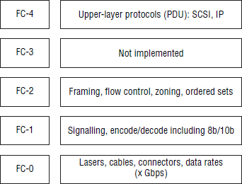
Because FCP is a simpler protocol, you will find yourself referring back to the FCP layers less often than you do for a TCP/IP network.

Just in case the IP network team try to you tell you that FCP's simplicity or fewer layers is some sort of shortcoming for FCP, it is not. It is actually a reflection of the fact that FCP is more of a channel technology than a network technology. Remember at the beginning of the chapter we explained that channels are low-overhead, low-latency, high-speed interconnects that attempt to re-create channels rather than massively complex networks.

FC Fabrics

A fabric is a collection of connected FC switches that have a common set of services. For example, they share a common name server, common zoning database, common FSPS routing table, and so on.

Most of the time you will want to deploy dual redundant fabrics for resiliency. Each of these two fabrics is independent of the other, as shown in Figure 5.10.

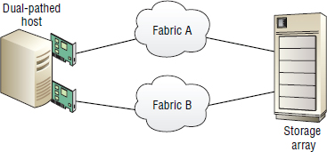
Each fabric is viewed and managed as a single logical entity. If you want to update the zoning configuration in the fabric, it is common across the fabric and can be updated from any switch in the fabric.

If you have two switches that are not connected to each other, each switch will run its own isolated fabric. If you then connect these two switches by stringing a cable between an E_Port on each switch, the fabrics will merge and form a single fabric. How this merging happens, and what happens to existing zoning configurations and principal switches, can be complicated and depends on the configuration of your fabrics. Before doing something like this, do your research and follow your vendor's best practices.

It is possible that two fabrics won't merge. When this happens, the fabrics are said to be segmented. Switches segmenting from fabrics can happen if certain important configuration parameters in each switch's configuration file do not match. Before merging fabrics, make sure that all switches in the fabric are configured appropriately.

Once the fabrics have merged, any device in the fabric can communicate with any other device in the fabric, as long as the zoning configuration allows it.

Fabric Services

All switches in a fabric support and participate in providing a common set of fabric services. As defined by FC standards, these fabric services can be reached at the following well-known FC addresses:

Not all of these fabric services are implemented, and from a day-to-day perspective, some are more important than others. Let's take a closer look.

The time server is responsible for time synchronization in the fabric. The management server allows the fabrics to be managed from any switch in the fabric. The zoning service is also a part of the management server. The fabric controller server is responsible for principal switch selection, issuing of registered state change notifications (RSCNs), and maintaining the Fabric Shortest Path First (FSPF) routing table. The fabric login server is responsible for issuing N_Port IDs and maintaining the list of registered devices on the fabric.

FC Name Server

The FC simple name server (SNS), better known these days as simply the name server, is a distributed database of all devices registered in the fabric. It is a crucial fabric service that you will interact with on a regular basis as part of zoning and troubleshooting.

All devices that join the fabric are required to register with the name server, making it a dynamic, centralized point of information relative to the fabric. As it is distributed, every switch in the fabric contains a local copy.

Targets and initiators register with, and query, the name server at the well-known address 0xFFFFFC.

Zoning

Device visibility in a SAN fabric is controlled via zoning. If you want two devices to be able to talk to each other, make sure they are zoned together!

Back to the original days of SCSI, when all devices were directly connected to a single cable inside a single server, that was a form of zoning—only that single server had access to the devices. Fast-forward to the days of shared SAN environments, where hundreds of targets and hundreds of initiators can talk to each other, and it's easy to see how this differs vastly from the original intent of SCSI. Something had to be done!

Fabric and Port Login

Before we dive into zoning, we'll cover some important background work on device discovery and the concept of fabric logins and port logins.

When an initiator first initializes on a SCSI bus, including an FC SAN, it performs a reset and then a discovery of all devices on the bus. In the case of a SAN, the bus is the SAN. On a SAN fabric with no zoning in place, the initiator will probe and discover all devices on the SAN fabric. As part of this discovery, every device will also be queried to discover its properties and capabilities. On a large SAN, this could take forever and be a massive waste of resources. But more important, it can be dangerous to access devices that other hosts are already using.

In order to speed up, smooth out, and generally improve the discovery process, the name server was created. Since the invention of the name server, each time any device joins the fabric, it performs a process referred to as a fabric login (FLOGI). This FLOGI process performs a bunch of important functions:

• Assigning devices their all-important 24-bit N_Port IDs
• Specifying the class of service to be used
• Establishing a device's initial credit stock

After a successful FLOGI process, the device then performs a port login (PLOGI) to the name server to register its capabilities. All devices joining a fabric must perform a PLOGI to the name server. As part of the PLOGI, the device will ask the name server for a list of devices on the fabric, and this is where zoning comes into play. Instead of returning a list of all devices on the fabric, the name server returns only a list of those devices that are zoned so as to be accessible from the device performing the PLOGI. Once the device performing the login has this list, it performs a PLOGI to each device in order to query each device's capabilities. This process is much quicker and more secure than probing the entire SAN for all devices, and it also allows for greater control and more-flexible SAN management.

Even with the preceding process, if no zoning is in place on the fabric, it is literally a free-for-all. Every device can see every other device, and you will find yourself in a very bad place.

Now let's take a closer look at zoning.

Zones

The basic element of zoning is the zone¸ and all SAN fabrics will contain multiple zones. Multiple zones are grouped together into a container know as a zone set.

As we've hinted already, zoning is a way of partitioning a fabric, with each individual zone being like a mini fabric, a subset of the wider fabric. If you want two devices to communicate with each other, put them in the same zone; all other devices should be excluded from that particular zone.

Figure 5.11 shows a simple SAN with two zones (Zone A and Zone B). In the figure, LegendaryHost can communicate with only LegendaryStorageArray, and at the same time, UberHost can communicate with only UberTapeLibrary. There are four devices on the fabric and two zones in operation—kind of like two mini fabrics.

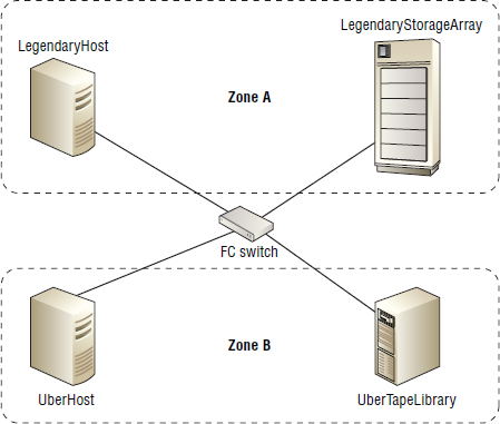
Although the example in Figure 5.11 is small, zoning scales to extremely large fabrics with potentially thousands of devices and thousands of zones. As in this example, zones are made up of initiators and targets. It is standard practice to give these initiators and targets friendly names, referred to as aliases, which can help immensely when troubleshooting connectivity issues.

Exercise 5.2 shows how to configure zoning.

Zoning Best Practices

The following rules of thumb regarding zoning will keep your SAN in good shape:

1. Keep zones small. This will make troubleshooting simpler.
2. Have only a single initiator in each zone. It is considered bad practice to have more than one initiator in a zone.
3. Keep the number of targets in a zone small, too. It is more acceptable to have multiple targets per zone than it is to have multiple initiators per zone. However, don't get carried away, as this can make troubleshooting more difficult.
4. Give your zones and aliases meaningful names.
5. Take great care when making zoning changes in your environments.

Of these best practices, the one that is probably the most important in the real world is point 2, referred to as single-initiator zoning. In a nutshell, single-initiator zoning states that every zone should contain only a single initiator plus any targets that the initiator needs to access. Live by this principle, and your life will be made a lot easier.

Zone Sets

Multiple zones are grouped together in to zone sets, and it is the zone set that is applied to the fabric. If you have configured a new zone, you will need to add it to the active zone set in order for it to be applied to the fabric.

It is possible for an FC fabric to have multiple defined zone sets. However, only a single zone-set can be active on any given fabric at any given time.

Aliases

We've briefly mentioned aliases, but let's have a closer inspection.

WWPNs are hideously long and mean nothing to the average human being. Aliases allow us to give friendly names to WWPNs on the SAN. Instead of having to remember that WWPN 50:01:43:80:06:45:d3:2f refers to HBA1 in our host called LegendaryHost, we can create an alias for that WWPN with a meaningful name.

The following command creates an alias called LegendaryHost_HBA1 in a Brocade fabric:

LegendarySw01:admin> alicreate LegedaryHost_HBA1 “50:01:43:80:06:45:d3:2f”

The following set of commands creates the same alias, but this time on a Cisco MDS fabric:

MDS-sw01# conf t
Enter configuration commands, one per line. End with CNTL/Z.
MDS-sw01 (config)# fcalias name LegendaryHost_HBA1
MDS-sw01 (config-fcalias)# member pwwn 50:01:43:80:06:45:d3:2f
MDS-sw01 (config-fcalias)# exit

Most people use aliases when configuring zoning, and it is a solid practice to stick to.

Port or WWN Zoning

There are two popular forms of zoning:

• WWN zoning
• Port zoning

Essentially, these are just two ways of identifying the devices you are zoning—either by WWPN or by the ID of the switch port the device is connected to.

Each approach has its pros and cons. If you go with port zoning and then have to replace a failed HBA in a host, you will not need to update the zoning as long as the new HBA remains cabled to the same switch port that the failed HBA was. However, if you implement WWN zoning, you will need to either update the alias and reapply the zone set to reflect the new WWPN of the new HBA or reset the WWPN on the new HBA to match that of the old HBA. In this respect, port zoning seems simpler. However, and this is massively important, the port ID used in port zoning can change! It is rare, but it can happen. This is because port IDs contain the domain ID of the switch, and the domain ID of a switch can change if the fabric ever has to perform a disruptive reconfiguration. If this ever does happen, you are staring down the barrel of invalid zoning and a lot of hard work to get things up and running again. For this reason, most people choose to go with WWN zoning. Also, from a ssecurity perspective, port zoning is considered more secure than WWN zoning due to the act that it isn't too hard to spoof a WWN, whereas it's more difficult to spoof which port you are connected to.

Hard Zoning or Soft Zoning

Soft zoning is basically name-server-enforced zoning.

When a device performs a PLOGI to the name server and requests a list of devices on the fabric, the name server returns only a list of devices that are in the same zones as the device performing the PLOGI. This way, the device logging in to the fabric gets a limited view of the fabric and should log in to only those devices. However, a bad driver in an HBA or CNA could decide to PLOGI to any or every possible device address on the fabric. If it did this, nothing would stop it. Therefore, soft zoning is nothing more than security by obscurity and relies on attached devices playing ball.

Both WWN and port zoning can be implemented as soft zoning.

In hard zoning, on the other hand, the switch hardware inspects all traffic crossing the fabric and actively filters and drops frames that are disallowed according to the zoning configuration. Name server zoning is still in effect—the name server still gives devices that are logging in a restricted view of the fabric—but hard zoning is also implemented as an additional level of security. The following command shows that on UberSw01, hard zoning is in place and we are using WWN zoning:

UberSw01:admin> portzoneshow
PORT: 0 (0)   F-Port    Enforcement: HARD WWN   defaultHard:   0   IFID: 0x44120b38
PORT: 1 (1)   Offline
PORT: 2 (2)   F-Port    Enforcement: HARD WWN   defaultHard:   0   IFID: 0x4412004b

Whether hard zoning is in place on your fabric is vendor specific and depends on how you have your fabric and zoning configured. Consult your vendor's best practices in order to deploy hard zoning.

SAN Topologies

Now let's cover SAN topologies and some of the principles, such as redundancy and high availability, that underpin them.

Redundancy

A hallmark of all good storage designs is redundancy.

Look at any storage design worth the paper it was written on, and you will see redundancy everywhere: servers with multiple HBAs, cabled to diverse redundant fabrics, connected to redundant storage processors; RAID-protected disks; replicated volumes; and the list goes on and on. This is essential because although there aren't usually that many bad days in the storage world, when those bad days do come along, they tend to be days from hell!

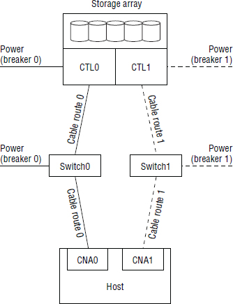
Almost every SAN environment in the world will have dual redundant fabrics—at least two fully isolated fabrics. These are isolated physically as well as logically, with no cables between them.

Figure 5.12 shows two redundant fabrics and identifies diverse cabling routes, power, and similar concerns.

Common SAN Topologies

There are several commonly recognized SAN topologies. These include point-to-point (FC-P2P), arbitrated loop (FC-AL), and the various switched fabric (FC-SW) topologies. We'll explore each of these next.

Point-to-Point

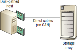
Point-to-point, referred to technically as FC-P2P, is a direct connection from a host HBA or CNA port to a storage array port. This connection can be a direct fly-lead connection or via a patch panel, but it cannot be via an FC switch.

FC-P2P is simple and offers zero scalability. If your storage array has eight front-end ports, you can have a maximum of eight directly attached servers talking to that storage array.

Figure 5.13 shows an FC-P2P connection.

Point-to-point configurations are most common in small environments where FC switches are not necessary and would unnecessarily increase costs.

Arbitrated Loop

Fibre Channel arbitrated loop, referred to as FC-AL, allows devices to be connected in a loop topology, usually via an FC hub. However, a hub is not required, as you can daisy-chain servers together in a loop configuration where the transmit port of one server is connected to the receive ports of the adjacent server.

FC-AL is a bit of a dinosaur technology these days and is rarely seen. This is good, because it lacks scalability (with a maximum of 127 devices) and performance.

In FC-AL configurations, all devices on the loop contend for use of the loop, and only a single device is allowed to transmit I/O on the loop at any point in time. This naturally leads to contention and drops in performance during periods of high activity.

FC-AL configurations also suffer from a phenomenon known as a LIP storm. Basically, any time a device is added to or removed from a loop, the loop reinitializes by sending loop initialization primitives (LIPs). During such reinitialization events, devices cannot transmit data on the loop. When FC-AL configurations were more commonly used, the bane of a storage administrator's life was having a flaky device on the loop that kept flooding the loop with LIP frames.

These days, FC-AL configurations mainly exist only in books like this or museums. R.I.P.

Switched Fabric

Fibre Channel switched fabric is technically referred to as FC-SW, but most people just call it fabric. It is the de facto standard in FC networking technology.

FC-SW overcomes all the limitations of FC-AL and FC-P2P, and adds a lot of improvements. As a result, this section presents it in more detail than FC-P2P and FC-AL.

A Fibre Channel fabric is made up of one or more FC switches. FC switches operate up to FC-2 layer, and each switch supports and assists in providing a rich set of fabric services such as the FC name server, the zoning database, time synchronization service, and more.

End devices can be added and removed from a fabric nondisruptively. Full nonblocking access to the full bandwidth of the fabric is provided to all devices. The fabric can scale to thousands of devices. The standards state millions of devices, but in practice this is thousands. Many FC switches operate in cut-through switching mode, which ensures the lowest possible latency by not having to buffer each frame in the switch as it passes through the switch.

When a fabric contains more than one switch, these switches are connected via a link known as an inter-switch link.

Inter-Switch Links

In order to connect two FC switches and form a common fabric—with a single instance of the name server and zoning table—you configure a port on each switch to be an E_Port and string a cable between these two ports. E_Ports are special ports used to connect two switches into a common fabric, and the link they form is called an inter-switch link, or ISL for short.

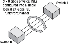
It is possible to run more than one ISL between two switches, and this is a common practice for redundancy. ISLs can operate as independent ISLs or can be bonded together to work as a single logical ISL. Generally speaking, bonding multiple physical ISLs into a single logical ISL is the preferred method, as this provides superior redundancy as well as superior load balancing across all physical links in the logical ISL.

Figure 5.14 shows three physical links bonded into a single logical ISL.

One important thing to consider when creating ISL PortChannels is deskew. Deskew refers to the difference in time it takes for a signal to travel over two or more cables. For example, it may take around 300 ns longer for a signal to travel over a 100-meter cable than it will a 10-meter cable. Deskew values are especially important when the logical ISL will cover long distances such as several miles. In such configurations, all physical cables forming the logical ISL need to have deskew values that meet your switch vendor's requirements. Not abiding by this rule will cause problems, such as the logical ISL not being able to form, or even worse, the logical ISL forming but performing poorly. The golden rule when it comes to ISL-related deskew values is always follow your switch vendor's best practices!

The following two commands show two physical ISLs formed into an ISL trunk between two Brocade switches. Each physical ISL is operating at 8 Gbps, creating a single logical ISL with 16 Gbps of bandwidth. Each physical ISL also has exactly the same deskew value—in our particular case, this is thanks to the fact that they are both running over short, 10-meter, multi-mode cables. It also shows that one of the physical ISLs in the trunk is the master. Not every vendor's implementation of logical ISLs has the concept of masters and subordinates, and having masters can be problematic if the master fails.

LegendarySw01:admin> islshow
  1: 14->14 10:00:00:05:AA:BB:CC:EE   03 LegendarySw03  sp:8G bw:16G  TRUNK QOS

LegendarySw01:admin> trunkshow
  1:14->14 10:00:00:05:AA:BB:CC:EE    21 deskew 15 MASTER
    15->15 10:00:00:05:AA:BB:CC:FF    21 deskew 15

The following command shows a similar logical ISL formed from two physical ISLs on a Cisco MDS switch:

MDS-sw01# show port-channel database
port-channel 10
    Administrative channel mode is active
    Operational channel mode is active
    Last membership update succeeded
    2 ports in total, 2 ports up
    Ports:   fc2/1    [up]*
             fc2/8    [up]

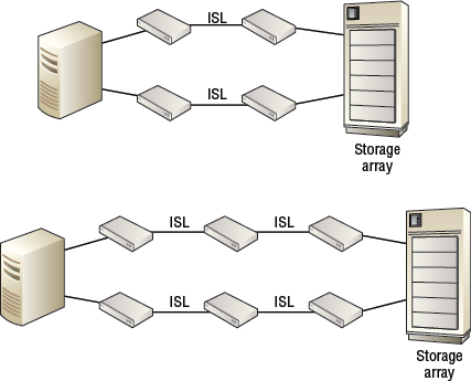
One final consideration regarding ISLs is hop count. Each ISL that a frame has to traverse en route from source N_Port to destination N_Port is referred to as a hop. If your initiator and target are patched to separate switches that are directly connected to each other via a single ISL, any communications between the two will have to traverse the ISL, resulting in one hop. If two ISLs have to be traversed, that equates to two hops. It is a good practice to keep your SAN as flat as possible and keep hop count to a minimum. That said, nodes attached to the fabric have no concept of how many switches exist in a fabric.

Figure 5.15 shows two simple configurations, one with a single hop and the other with two hops required.

Within FC-switched fabrics, there are several loosely accepted topologies. By far the most popular is the core-edge topology. Other designs (such as cascade, ring, and mesh) do exist, but are rare compared to the almost ubiquitous core-edge. Let's have a close look at each.

Before we look at some of the topologies, it is worth pointing out that when referring to a fabric topology, we are referring to switches and ISLs only. Moving an end device such as a host or storage array from one switch port to another, or even from one switch to another switch, does not usually affect the topology of the fabric. The notable exception is in a tiered topology.

Core-Edge Topology

The core-edge topology is by far the most widely implemented topology, and it will suit most requirements. A core-edge fabric looks a lot like an old hub-spoke, or a star network topology. You have a core switch at the physical center of the fabric, and each edge switch connects to the core switch via ISLs. Figure 5.16 shows a core-edge design with a single director at the core, and six edge switches connecting to the core.

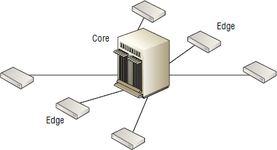
The core-edge design naturally lends itself to blade server environments whereby small SAN- or FCoE-capable switches are embedded in the blade server chassis. ISLs then run from these embedded-edge switches to a core switch, where the storage is directly connected.

It is perfectly acceptable for a core-edge design to have more than one core switch per fabric, as shown in Figure 5.17.

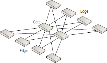
As far as fabric services are concerned, there is nothing special about the core switch. However, many people choose to force the core switch to be the principal switch in the fabric, as well as opting to perform most of the fabric management from the core switch. This does not have to be the case, though. However, having the core switch as the principal switch is a good idea because it is the switch least likely to be rebooted.

Cascade Topology

Cascaded designs connect switches in a row, as shown in Figure 5.18.

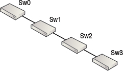
Cascade topology is an abomination, and 99.999 percent of the time should not be deployed, as it is not scalable, performant, or reliable. If switch 2 (Sw2) in Figure 5.18 fails, switch 3 (Sw3) is isolated from the rest of the fabric.

Ring Topology

Ring topology is the same as cascade except that the two end switches are connected, making it ever so slightly less hideous than cascade topology. By linking the two end switches, you offer an alternative path to a destination by sending frames in the opposite direction around the ring. Obviously, if a switch in a ring design fails, the topology becomes a cascade, but devices do not become isolated, because of the alternative path. However, adding switches to a ring topology requires the ring to be broken.

Like cascade, it is not a popular design and has few if any practical use cases in the modern storage world.

Mesh Topology

Mesh topologies have every switch in a SAN connected to every other switch. This ensures that every switch is only a single hop away from any other switch and is highly resilient and performant. However, it is extremely costly from an ISL perspective. Basically, lots of switch ports get used up as ISLs. Figure 5.19 shows a simple mesh topology.

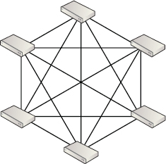
Mesh topologies are increasingly wasteful of ports (because they need to be used as ISLs) as they scale.

Tiered Topologies

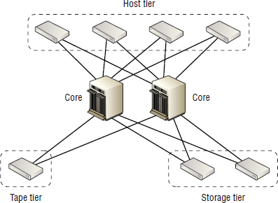
Tiered topologies are the enemy of localization. In a tiered fabric topology, you group all like devices on the same switch. For example, all hosts would go on a set of switches, all storage ports on a set of switches, all tape devices on a set of switches, and all replication ports on a set of switches. This design guarantees that hosts accessing storage or tape devices have to cross at least one ISL. This is not the end of the world, though, as long as you have sufficient ISL bandwidth.

Maintenance and expansion of tiered fabric designs is extremely simple compared to extreme localization. In a tiered design, it is relatively simple to increase bandwidth between tiers by simply adding ISLs. It is also easy to expand a tier by adding more switches or more switch ports to it.

In the real world, tiered fabric topologies are fairly common, especially if you consider placing all storage and tape devices on core switches and all hosts on edge switches in a hybrid tiered core-edge topology.

Figure 5.20 shows a simple core-edge fabric design that incorporates a form of tiering.

Despite all of this talk about topologies, it is not a requirement to design a fabric around any specific topology. You can mix and match and tweak a design to your requirements.

FC Routing

Now let's look at how frame delivery and routing works in FC fabrics, as well as some vendor implementations of virtual fabrics and virtual SANs.

Virtual Fabrics and VSANS

The two major FC switch vendors—Brocade and Cisco—have technologies that allow you to partition physical switches to the port level, allowing individual ports in a single physical switch to belong to discrete fabrics.

Cisco invented the technology and refers to it as virtual SAN (VSAN). The ANSI T11 committee liked it so much that they adopted it as an industry standard for virtual fabrics. Brocade then based its virtual fabrics implementation on the ANSI T11 standard. As a result, it shouldn't be much of a surprise that Cisco's VSAN and Brocade's virtual fabrics technologies are extremely similar.

Cisco VSAN

Each VSAN is a fully functioning fabric, with its own dedicated ports, devices, and fabric services. These fabric services include the usual suspects of the name server, zoning table, alias table, and so on.

All F_Ports on Cisco MDS and Nexus FCoE switches can be a member of one, and only one, VSAN. However, ISLs—including PortChannels—in trunk mode can carry traffic for multiple VSANs while maintaining isolation of traffic from the different VSANs. They do this by virtue of a VSAN tag that is added to the FC frame header to identify VSAN membership.

A good use case for VSANs might include partitioning the ports on a single switch into a development fabric and a staging fabric. This would allow you to have a single physical platform running two distinct, isolated, logical fabrics. You can dynamically move ports between the development and staging fabrics as required, allowing for good flexibility. If you mess up the zoning in the development fabric, the staging fabric will be unaffected. It works great, and you no longer need to buy dedicated hardware if you want to isolate fabrics!

While separating ports on isolated logical fabrics (VSANs), it is possible to route FC frames between devices on separate VSANs via a Cisco technology referred to as inter-VSAN routing (IVR). IVR works by creating zones and adding them to the IVR zone set. Zones in the IVR zone set effectively overlap VSANs, allowing devices that are in separate VSANs but exist in the IVR zone set to communicate with each other.

Brocade Virtual Fabrics

Brocade virtual fabrics are essentially the same as Cisco VSANs. They allow you to carve up physical switches by allocating ports to newly created logical switches. Multiple logical switches then form logical fabrics, each of which has its own separate fabric services—name server, zoning, domain IDs, principal switches, and the like.

Use cases are the same as with Cisco VSANs. Take a single physical piece of tin, carve its resources into discrete logical entities that can be managed separately, and maintain traffic isolation between the logical entities. Again, mess up the zoning DB on a Brocade logical fabric, and all other logical fabrics remain unaffected.

As with Cisco VSAN technology, it is possible to route traffic between logical fabrics by using Brocade's Fibre Channel Routing (FCR) technology and Logical Storage Area Network (LSAN) zones. However, the Brocade FCR technology requires a special base switch to act as a backbone fabric that enables routing between two separate fabrics.

FC Naming

Every end device on an FC SAN has two important identifiers:

• World wide name
• Node port ID

As a storage guy, you will interact with world wide names and world wide port names more often than you will interact with N_Port IDs.

World Wide Names

Each node port—host HBA/CNA port, storage array port—has its own 64-bit (8-byte) worldwide unique number that stays with its device for its entire life. This 64-bit name is known as a world wide name (WWN). Actually, each node port has a world wide node name (WWNN) and a world wide port name (WWPN). More often than not, you will work with WWPNs.

The world wide port name is sometimes referred to as a port world wide name, or pWWN. This book uses the term WWPN.

The following output from a switchshow command on a Brocade FC switch shows the switch's WWNN as well as the WWPNs of the end devices connected to the first two FC ports in the switch (as mentioned, you cannot address traffic to the switch by its WWN):

LegendarySw01:admin> switchshow
SwitchNAme:   LegendarySw01
SwitchType:   62.3
SwitchState:  Online
SwitchMode:   Native
SwitchRole:   Principal
SwitchDomain: 44
SwitchId:     fffXXX
SwitchWwn:    10:00:00:05:AA:BB:CC:DD
Zoning:       ON (Prd_Even1)
SwitchBeacon: OFF

Index Port Address Media Speed State     Proto
==============================================
  0   0    220000  cu    8G    Online    FC  F_Port 50:01:43:80:be:b4:08:62
  1   1    220100  cu    8G    Online    FC  F_Port 50:01:43:80:05:6c:22:ae

The following nsshow command shows the WWNN and WWPN of a host HBA:

LegendarySw01:admin> nsshow
Type Pid    COS     PortName                NodeName                TTL(sec)
N    220100;  3;    50:01:43:80:05:6c:22:ae;50:01:43:80:05:6c:22:af  na
    FC4s: FCP
    NodeSymb: [43] “QMH2462 FW:v5.06.03 DVR:v8.03.07.09.05.08-k”
    Fabric Port Name: 10:00:00:05:AA:BB:CC:DD
    Permanent Port Name: 50:01:43:80:05:6c:22:af
    Port Index: 1
    Share Area: No
    Device Shared in Other AD: No
    Redirect: No
    Partial: No

WWNs—both WWNN and WWPN—are manufacturer assigned. WWNs are written as 16 hexadecimal digits, with every two digits being separated by a colon. WWNs can contain only hexadecimal characters and are therefore not case sensitive, meaning that 50:01:43:80:05:6c:22:af and 50:01:43:80:05:6C:22:AF are identical.

WWNs are burned into the HBA/CNA card, similar to the way a MAC address is burned into a NIC. However, that should be where the MAC address analogy stops! Unlike MAC addresses, WWNs are not used for transporting frames on the fabric. It is the 24-bit N_Port ID (covered later in this chapter) that is used for frame routing and switching.

WWNs are used primarily for security-related actions such as zoning and other device security, which are also covered in detail later.

N_Port IDs

As we mentioned earlier, WWNs are not used for frame switching and delivery on FC networks. This is where N_Port IDs come into play.

Before exploring an N_Port ID, let's look at what an N_Port is. N_Port is FC lingo for node port, and it refers to physical FC ports in end devices on FC networks. Basically, all storage array ports and host HBA ports are end points and therefore are considered N_Ports. FC switches, on the other hand, do not act as end points and therefore do not have N_Ports. N_Ports apply to only FC-P2P and FC-SW architectures. But these are just about the only topologies being deployed these days anyway.

Some people refer to N_Port IDs as Fibre Channel IDs, or FCIDs for short. You can use either term. This book uses N_Port ID.

An N_Port ID is a 24-bit dynamically assigned address. It is assigned by the fabric when an N_Port logs in to the fabric. Every end point in the fabric has one, and it is this N_Port ID that is coded into the FC frame header and used for frame switching, routing, and flow control.

Let's take another look at a switchshow output and highlight the N_Port ID of the connected devices in bold:

LegendarySw01:admin> switchshow
SwitchNAme:   LegendarySw01
SwitchType:   72.3
SwitchState:  Online
SwitchMode:   Native
SwitchRole:   Principal
SwitchDomain: 44
SwitchId:     fffXXX
SwitchWwn:    10:00:00:05:AA:BB:CC:DD
Zoning:       ON (Prd_Even1)
SwitchBeacon: OFF

Index Port Address Media Speed State     Proto
==============================================
  0   0    220000  cu    8G    Online    FC  F_Port 50:01:43:80:be:b4:08:62
  1   1    220100  cu    8G    Online    FC  F_Port 50:01:43:80:05:6c:22:ae

N_Port IDs are smaller than WWPNs and are included in every frame header, which allows for smaller frame headers than if WWNs were used for frame routing and end-to-end delivery.

Also, just to be clear, a device with two physical ports connected to a SAN will get two N_Port IDs, one for each port.

The format and structure of N_Port IDs is as follows:

Domain The first 8 bits of the address are known as the domain ID. This can be a value from 1–239, and it is the domain ID of the switch the port belongs to.

Area This is the next 8 bits, and the switch vendor assigns and structures this part of the address. The value in this section of the N_Port ID can be anything from 0–255.

Port The last 8 bits of the address are also vendor specific and usually translate to the port number of the port in the switch. The value can be anything from 0–255, and switches with more than 256 ports use a combination of area and port to uniquely identify the port.

This hierarchical nature of N_Port IDs assists with frame routing and delivery. It is only the domain portion of the N_Port ID that is used in routing decisions until the frame reaches the destination switch.

N_Port ID Virtualization

Originally, a physical N_Port logged in to a fabric and got a single N_Port ID back from the fabric login server. Things were nice and simple. However, with the emergence of server virtualization technologies, it became desirable for a physical N_Port to be able to register multiple N_Ports and get back multiple N_Port IDs so that an N_Port ID could be assigned to a virtual machine, and the SAN zoning could limit access to some resources to that VM alone. Witness the birth of N_Port ID virtualization (NPIV).

Before the days of NPIV, an N_Port would perform a FLOGI to obtain an N_Port ID from the fabric and then perform a PLOGI to register its N_Port ID with the name server. Job done. Fast forward to today, and a node supporting NPIV registers multiple virtual N_Ports with the fabric. Registration of additional N_Ports on the fabric is not done via more FLOGI operations, though. It is done via FDISC operations. Basically, an N_Port can perform as many FDISC operations as it wishes, with each FDISC followed by a PLOGI for the acquired N_Port ID. Figure 5.21 shows a single host with a single physical HBA that has registered an additional four N_Port IDs with the fabric.

In order to get additional N_Port IDs for each virtual N_Port, the FDISC operation registers an additional WWPN with the fabric. This means that NPIV-capable devices have to have multiple WWPNs—one for each N_Port ID it wants. Also, in order for NPIV to work, the fabric and switches obviously have to support NPIV. Otherwise, they will get confused when they see multiple N_Port IDs and WWPNs originating from a single host connected to a single F_Port.

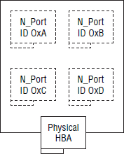
Generally speaking, on the HBA/CNA side of things, NPIV-aware HBAs are capable of carving themselves up into multiple virtual HBAs. Each virtual HBA has its own WWPN and can therefore register for its own N_Port ID as if it were a fully fledged physical N_Port. This allows each virtual HBA to be directly addressed on the fabric. Couple this with the ability to associate a virtual HBA with a VM, and bingo, you have a VM that is directly addressable on the fabric and can have storage presented directly to it.

Figure 5.22 shows two LUNs presented directly to the WWPNs that are associated with two VMs in a single server behind a single physical HBA.

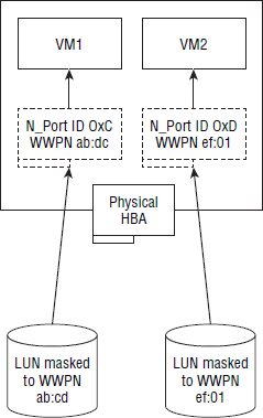
Of course, mapping LUNs directly to VMs and bypassing the hypervisor is not universally liked, nor is it appropriate for all situations. But it definitely has its place.

NPV and Access Gateway Modes

First up, NPV is not the same as NPIV. It looks the same, and it's based on NPIV, but it's not the same thing!

NPV is an abbreviation for N_Port Virtualizer, and as a technology, the main goal of NPV is to enable switches from multiple vendors to coexist in the same fabric without having to resort to nasty interop modes. NPV also allows you to have lots of switches in a fabric without overloading the fabric services and depleting the finite number of supported switches—actually, the finite number of domain IDs—in a fabric.

It is time for a bit of background as to why NPV is so cool.

When an FC switch joins a fabric, it gets its own unique Domain_ID. It also participates in a load of fabric services, some of which we have discussed. As you add more and more switches to a fabric, you start to approach scalability limitations such as maxing out the number of supported domain IDs in a fabric. NPV helps here. We'll explain how in a second.

Also, if you build a fabric by using switches from Cisco, Brocade, and QLogic, you are going to have to get down with some funky interop mode madness and end up with a fabric with a very limited feature-set that is going to be a support headache from day one. NPV comes to the rescue here too.

So, the secret behind NPV is that a switch in NPV mode is invisible to the fabric. It doesn't register for a domain ID and it doesn't share the burden of assisting with fabric services. As far as the fabric is concerned, the switch is not a switch; it just looks like an N_Port running NPIV (yes, NPIV, not NPV).

A common use case is running NPV switches at the edge and leaving the core switches to take care of all of the fabric services. This is popular in situations where customers are adding Cisco UCS blade servers to environments that already operate Brocade or QLogic fabrics. Edge to core appears to be the sweet spot for NPV, and you wouldn't want to have to use it between core switches over a long distance.

Interestingly, the links between switches running NPV are not ISLs, and the ports are not E_Ports. The ports on the edge switch are sometimes referred to as NP_Ports, and the ports on the core switches are just normal F_Ports.

Also of interest is that the NPV switches on the edge effectively proxy all of the FLOGI and PLOGI operations from the end devices connected to them. The NPV switch on the edge performs a FLOGI and PLOGI to the core switch for itself. It then converts FLOGIs from connected hosts to FDISCs and proxy registers each end device with the core as per NPIV. This way, the core switch just thinks it's talking to an NPIV node over a standard F_Port. It is simple and effective.

NPV is a standards-based technology, which is better than interop modes ever were. The result is good support between vendors. Interop mode is dead; long live NPV!

There are a couple of things to be aware of. Load balancing and HA of links from edge to core can vary between vendors. Load balancing tends to be basic round-robin, but this may change in the future. Also, be sure to check with your vendors about support of VSAN and virtual fabric technologies, especially trunking VSANs over connections between edge and core switches operating in an NPV configuration.

To see whether NPV/AG mode is enabled on a switch, issue the following commands:

LegendarySwitch01:admin> ag --modeshow
Access Gateway mode is enabled

The following output on a Cisco MDS fabric shows two switches that are configured in NPV mode in VSAN 8:

MDS-sw01# show fcns database
VSAN 8:
--------------------------------------------------------------------------
FCID TYPE PWWN (VENDOR) FC4-TYPE:FEATURE
--------------------------------------------------------------------------
0x010000 N 20:01:00:0d:ec:AA:BB:CC (Cisco) npv
0x010001 N 20:02:00:0d:ec:AA:BB:CD (Cisco) npv

Framing

Fibre Channel is essentially a unicast frame-based protocol. Most of what goes on in an FC SAN can be viewed as traditional layer 2 networking. FC frames can be up to 2,148 bytes long and can contain a payload of up to 2,112 bytes that must be divisible by 4.

Figure 5.23 shows an FC frame.

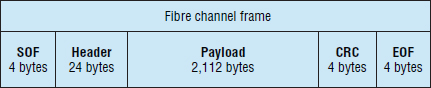
Now let's explain each component of the frame, starting at the left and working our way to the right.

Start of Frame All FC frames are prefaced with a start of frame (SOF) ordered set that acts as a form of frame delimiter. The SOF is a single 4-byte word indicating the class of service (COS) and at what point this particular frame figures in a set.

Header Directly following the SOF is a 24-byte frame header. This contains the source and destination N_Port IDs, referred to as source ID (SID) and destination ID (DID). The header also defines whether the frame contains user data (data frame) or control data (link control frame) and indicates where a frame is featured in an exchange or sequence.

Payload Following the header comes the payload. This can be up to 2,112 bytes long and must be padded if not divisible by 4.

Cyclic Redundancy Check Frame integrity is possible via a cyclic redundancy check (CRC).

End of Frame Last but not least comes the end of frame (EOF) ordered set. This informs the receiving node that the frame is ended, and the specifics of the EOF are determined by the class of service of the frame.

The preceding is good theory, but it is unlikely that you will need to call upon such knowledge very often in your day-to-day storage administration.

Flow Control

First you need to know a bit of background before we jump into the specifics of flow control. At a fairly high level, communication on an FC SAN is composed of three basic constructs: frames, sequences, and exchanges. The smallest and most fundamental unit is the frame. Multiple related frames form a sequence, and multiple related sequences form an exchange. A conversation is frequently used as an analogy. In this analogy, frames are words, sequences are sentences, and exchanges are conversations. That is good to know, but you probably won't rely on that knowledge every day in your job.

Flow control in an FC SAN is based on a credit system. End devices are issued with credits and are allowed to send one frame for every credit that they have. If there are no credits, no frames can be sent! This approach works fairly well for avoiding congestion and frame dropping.

There are two major credit systems in use:

• Buffer to buffer (B2B)
• End to end (E2E)

B2B credit works between two directly connected ports such as an end device and a switch port (N_Port to F_Port). E2E credit works between two end devices such as an initiator and a target.

End-to-End vs. Buffer-to-Buffer Flow Control

E2E flow control (sometimes referred to as EE_credit) works on the principle of the destination device returning an Accept (ACC) to the sender to indicate that it has received a frame and that the sender can increment its credit stock by one. Each time the sender sends a frame, it decreases its credit stock by one, and each time it receives an ACC, it increments its credit stock by one. This ACC-based replenishing scheme works with class of service 1 and class of service 2 because they both work on the principle of end-to-end connectivity and use acknowledgments. These acknowledgments allow the sender to maintain a rolling stock of credits. Switches have no involvement in E2E credit schemes.

B2B flow control (sometimes called BB_credit) works between node ports and fabric ports. As B2B is used by COS 3, which is connectionless without acknowledgments, ACC frames are not used to replenish credits. Instead, a special receiver ready frame (R_RDY) is issued back to the sender to indicate that the recipient is ready to receive more frames. Similar to E2E, in a B2B credit system, the sender decreases its credit stock by one for every frame it sends and increases it by one for every R_RDY it receives.

Both E2E and B2B credit systems require the sender to have an initial stock of credits. This credit stock is agreed at FLOGI for B2B and at PLOGI for E2E. This initial credit stock is important because if a device started life in a fabric without any credits, it would never be able to send frames.

Since we're on the topic, I suppose there is no harm in mentioning that arbitrated loop (FC-AL) environments support a form of B2B credit system. However, in this situation, each device works with an initial credit of zero. Once an initiator arbitrates control of the wire, it contacts the target, which responds with a number of R_RDYs representing the number of credits it wishes the initiator to have.

Error Recovery

FC frame recovery works at the sequence level, meaning that if a frame is dropped or lost, the entire sequence must be re-sent. This isn't the end of the world, because most FC SANs are stable and not congested, meaning that recovery isn't required very often.

Flow Control over Long Distances

In stretched or extended fabric configurations, switch ports at either end of the long-distance link are configured with extra buffers to allow more frames to be sent and exist on the link without having to wait for acknowledgments.

Generally speaking, the longer the distance between the sending and receiving port, the more credits are assigned to the port. If additional credits weren't assigned, the effective bandwidth of these links would be reduced as the sender waited for R_RDY frames, due to the bandwidth-delay product. Also, data can be sent on the transmit line and credits can be replenished on the receive line in full-duplex mode.

Classes of Service

In an attempt to provide differing levels of service—basically, delivery guarantees and bandwidth consumption—the FC Protocol defines seven classes of service (COS). However, not only are they not all implemented, the vast majority of FC traffic is either Class 3 or Class F, with a smattering of Class 2 occasionally seen in the real world.

Class 1

Class 1 is a connection-oriented link that uses acknowledgments. While it isn't widely implemented, you may see it on an exam. In Class 1 connections, the initiator and target consume the full bandwidth of the link and maintain a virtual circuit until the transmission sequence ends. Acknowledgment frames are used to ensure reliable and in-order frame delivery. Class 1 connections use only E2E flow control.

Class 2

Class 2 is a connectionless link that uses acknowledgments. It's kind of similar to TCP, if you know your TCP/IP theory. Basically, it is not a dedicated connection but requires delivery acknowledgments. Class 2 connections can request in-order frame delivery, but it is not mandatory. Out-of-order frame delivery in FC SANs is rare compared to Ethernet networks.

Class 2 connections use both E2E and B2B flow control. Class 2 is seen more often than class 1, but still not very often.

Class 3

Class 3 is a connectionless service that does not use acknowledgment frames. This is easily the most common class of service seen in FC fabrics and is conceptually similar to UDP in the TCP/IP world. If you know your TCP/IP theory, due to its similarity with UDP, COS 3 is sometimes referred to as a datagram service.

Generally speaking, FC SAN environments do not drop or discard frames, meaning that acknowledgment frames are an unnecessary overhead—unless, of course, you utilize these ACC frames to replenish credits. If frames are dropped, it is the responsibility of the upper-layer protocols to clean up the mess and ensure retransmission.

Class 3 uses only B2B flow control.

Class 4

Class 4 defines a connection-based service with acknowledgments. It differs from class 1 in that it consumes fractional bandwidth and can apply quality of service to connections. However, it is rarely implemented.

Class F

Class F is a lot like class 2. It is connectionless but utilizes acknowledgment frames. Class F is the de facto COS used for switch-to-switch communications. It operates only across E_Ports and ISLs. It is used for delivery of control data such as state-change notifications, name server updates, routing info, zoning, build fabric requests, and reconfigure fabric requests. Class F uses the B2B flow control mechanism.

Oversubscription

Oversubscription occurs when more than one device utilizes a single link. ISLs are often oversubscribed. For example, an edge switch with 24 8 Gbps ports may be configured as follows:

• 22 hosts each connected at 8 Gbps
• 2 ISL ports configured as a single 16 Gbps ISL to the core switch

In order for the 22 hosts to access the storage array connected to the core switch, all 22 hosts have to cross the 16 Gbps ISL. If all 22 hosts utilized their full 8 Gbps, the ISL would be a severe bottleneck. However, if you know that the combined throughput of all your hosts will never push anywhere near the maximum theoretical throughput of their 8 Gbps, you can safely oversubscribe your ISL as described.

If all ports in a fabric operate at the same speed, oversubscription is simply the ratio of node ports to ISLs. So if you have 10 hosts at 8 Gbps, and a single ISL at 8 Gbps, you have an oversubscription ratio of 10:1. However, in the previous example, we have a logical ISL operating at 16 Gbps and 22 hosts operating at a theoretical 8 Gbps each, so our oversubscription ratio would be 11:1.

Oversubscription isn't just used for ISLs. It is also common for a single storage port to be zoned with multiple hosts in a fan-out configuration. For example, a single storage port might be zoned with 10 host ports in a 1:10 fan-out ratio. If the hosts and storage port are operating at the same speed, we have a 10:1 oversubscription ratio. Again, this is extremely common in the real world because 99 percent of the time hosts do not, and cannot, drive their full bandwidth. This is especially so when you consider that most hosts will have multiple active links (for redundancy).

Locality

Locality is the degree to which communication between two devices is kept as close as possible. For example, two communicating devices connected to the same switch have a high degree of locality. In contrast, two devices that are on separate switches three hops apart have a very low degree of locality.

Locality can help avoid congestion by sticking storage and hosts close to each other, but don't get carried away with it. It is perfectly acceptable to have hosts attached to edge switches, and storage attached to core switches. This is common in blade server configurations, where there are embedded edge switches in the blade server chassis.

Fabric Reconfigurations

Certain fabric-related events can cause a fabric to reconfigure. Some of these events include the following:

• New switches added to the fabric.
• Merging fabrics.
• A new principal switch is selected.

There are two types of fabric reconfigure events:

• Build fabric (BF)
• Reconfigure fabric (RCF)

Build fabric events are nondisruptive, but reconfigure fabric events are disruptive.

During an RCF event, a principal switch election is held, domain IDs are assigned, and routes are established. It is entirely possible that the same principal switch will be reelected, and that domain IDs will not change. However, if they do change, this can be a pain in the neck, especially if you are using port zoning.

For these reasons, it is obviously preferred to perform a BF rather than an RCF.

FC SAN Troubleshooting

As you have seen, there are a lot of ways you can handle FC SAN. Consequently, there are a lot of areas where you can experience trouble with your configurations. Let's take a look at some of the ways you can troubleshoot FC SAN.

Backing Up Your Switch Configurations

While not exactly troubleshooting, you should make regular backups of your switch configurations, just in case you are ever in a situation where things are fouled up beyond all repair (FUBAR) and you have to revert to a previous configuration. Such backup files tend to be human-readable flat files that are extremely useful if you need to compare a broken configuration image to a previously known working configuration. Another option might be to create a new zone configuration each time you make a change, and maintain previous versions that can be rolled back to if there are problems after committing the change.

Troubleshooting Connectivity Issues

Many of the day-to-day issues that you will find yourself troubleshooting include connectivity issues such as hosts not being able to see a new LUN or not being able to see storage or tape devices on the SAN. More often than not, connectivity issues will be due to misconfigured zoning.

Each vendor provides different tools to configure and troubleshoot zoning, but the following common CLI commands can prove very helpful.

fcping

fcping is an FC version of the popular IP ping tool. fcping allows you to test the following:

• Whether a device (N_Port) is alive and responding to FC frames
• End-to-end connectivity between two N_Ports
• Latency
• Zoning (some implementations check zoning between two devices)

fcping is available on most switch platforms as well as being a CLI tool for most operating systems and some HBAs. It works by sending Extended Link Service (ELS) echo request frames to a destination, and the destination responding with ELS echo response frames.

The following fcping command is run on a Brocade switch and proves that a device is alive and responding to FC frames:

LegendarySw01:admin> fcping 50:01:43:80:05:6c:22:ae
Pinging 50:01:43:80:05:6c:22:ae [0x 220100] with 12 bytes of data:
received reply from 50:01:43:80:05:6c:22:ae: 12 bytes time:1162 usec
received reply from 50:01:43:80:05:6c:22:ae: 12 bytes time:1013 usec
received reply from 50:01:43:80:05:6c:22:ae: 12 bytes time:1442 usec
received reply from 50:01:43:80:05:6c:22:ae: 12 bytes time:1052 usec
received reply from 50:01:43:80:05:6c:22:ae: 12 bytes time:1012 usec
5 frames sent, 5 frames received, 0 frames rejected, 0 frames timeout
Round-trip min/avg/max = 1012/1136/1442 usec

The following fcping command is run to the same WWPN when the device is not alive on the network:

LegendarySw01:admin> fcping 50:01:43:80:05:6c:22:ae
Pinging 50:01:43:80:05:6c:22:ae [0x 220100] with 12 bytes of data:
Request timed out
Request timed out
Request timed out
Request timed out
Request timed out
5 frames sent, 0 frames received, 0 frames rejected,5 frames timeout
Round-trip min/avg/max = 0/0/0 usec

The following command shows the same host being fcpinged, but this time from a Linux host on interface n0.170 and specifying the N_Port ID instead of the WWPN:

fcping -c 3 -h n0.170 -F 0x220100
sending echo to 0x220100
echo    1 accepted                     16.170 ms
echo    2 accepted                      7.053 ms
echo    3 accepted                      6.803 ms
3 frames sent, 3 received 0 errors, 0.000% loss, avg. rt time 10.009 ms

Some switch vendors also check the zoning table when you specify two N_Port IDs in the same fcping command. For example, the following fcping command on a Brocade switch checks the zoning table to ensure that the two WWPNs specified are correctly zoned to each other:

LegendarySw01:admin> fcping 50:01:43:80:be:b4:08:62 50:01:43:80:05:6c:22:ae
Source: 50:01:43:80:be:b4:08:62
Destination: 50:01:43:80:05:6c:22:ae
Zone Check: Not Zoned

fctrace

Another tool that is modeled on a popular IP networking tool is the fctrace tool. This tool traces a route/path to an N_Port. The following command shows an fctrace command on a Cisco MDS switch:

MDS-sw01# fctrace fcid 0xef0010 vsan 1
Route present for :  0xef0010
20:00:00:05:30:00:59:ba(0xfffbee)
Latency: 0 msec
20:00:00:05:30:00:58:1b(0xfffc6b)
Timestamp Invalid.
20:00:00:05:30:00:59:1e(0xfffcef)
Latency: 174860 msec
20:00:00:05:30:00:58:1b(0xfffc6b)

Brocade has a similar tool called pathinfo.

While on the topic of zoning, these are some good things to consider:

• Are your aliases correct?
• If using port zoning, have your switch domain IDs changed?
• If using WWPN zoning, have any of the HBA/WWPNs been changed?
• Is your zone in the active zone set?

Rescanning the SCSI Bus

After making zoning changes, LUN masking changes, and pretty much any other work that changes a LUN/volume presentation to a host, you may be required to rescan the SCSI bus on that host in order to detect the new device. The following command shows how to rescan the SCSI bus on a Windows server using the diskpart tool:

DISKPART> list disk

  Disk ###  Status         Size     Free     Dyn  Gpt
  --------  -------------  -------  -------  ---  ---
  Disk 0    Online           68 GB      0 B
  Disk 1    Online          140 GB  1024 KB
  Disk 2    Online          100 GB  1024 KB

This output shows three volumes. However, we have just presented a fourth volume to this host that is not showing up. To rescan the SCSI bus, we will issue a rescan command:

DISKPART> rescan

Please wait while DiskPart scans your configuration…

DiskPart has finished scanning your configuration.

Now that we have issued the rescan, the following list disk command now shows all four devices:

DISKPART> list disk

  Disk ###  Status         Size     Free     Dyn  Gpt
  --------  -------------  -------  -------  ---  ---
  Disk 0    Online           68 GB      0 B
  Disk 1    Online          140 GB  1024 KB
  Disk 2    Online          100 GB  1024 KB
  Disk 3    Online          250 GB   250 GB

If you know that your LUN masking and zoning are correct but the server still does not see the fourth device, it may be necessary to reboot the host.

Understanding Switch Configuration Dumps

Each switch vendor also tends to have a built-in command/script that is used to gather con-figs and logs to be sent to the vendor for their tech support groups to analyze. The output of these commands/scripts can also be useful to you as a storage administrator. Each vendor has its own version of these commands/scripts:

Let's look at a cut-down example of a show tech-support brief on a Cisco MDS switch. From the truncated output, you can see that the switch has two configured VSANs and lists two ports, one configured in each VSAN. You can also see other interesting information, such as the management IP address, firmware version, and so on:

MDS-sw01# show tech-support brief
Switch Name           : MDS-sw01
Switch Type           : DS-X9216-K9
Kickstart Image       : 1.3(2) bootflash:///m9200-ek9-kickstart-mz.1.3.1.10.bin
System Image          : 1.3(2) bootflash:///m9200-ek9-mz.1.3.1.10.bin
IP Address/Mask       : 10.10.10.101/24
Switch WWN            : 20:00:00:05:30:00:75:32
No of VSANs           : 2
Configured VSANs      : 1,9

VSAN    1:    name:VSAN0001, state:active, interop mode:default
              domain id:0x6d(109), WWN:20:01:00:05:30:00:84:9f [Principal]
              active-zone:VR, default-zone:deny

-------------------------------------------------------------------------------
Interface  Vsan   Admin  Admin     Status        FCOT  Oper   Oper   Port
                  Mode   Trunk                         Mode   Speed  Channel
                         Mode                                 (GBps)
-------------------------------------------------------------------------------
-------------------------------------------------------------------------------
Interface  Vsan   Admin  Admin     Status        FCOT  Oper    Oper   Port
                  Mode   Trunk                         Mode    Speed  Channel
                         Mode                                  (GBps)
-------------------------------------------------------------------------------
fc1/1      1      auto   on        fcotAbsent     --    --              --
fc1/2      9      auto   on        fcotAbsent     --    --              --

<output truncated>

Using Port Error Counters

Switch-based port error counters are an excellent way to identify physical connectivity issues such as these:

• Bad cables (bent, kinked, or otherwise damaged cables)
• Bad connectors (dust on the connectors, loose connectors)

The following example shows the error counters for a physical switch port on a Brocade switch:

LegendarySw01:admin> portshow 4/15
portName: LegendaryHost_HBA1
portHealth: HEALTHY


......
portFlags: 0x24b03       PRESENT ACTIVE F_PORT G_PORT U_PORT LOGICAL_ONLI
portType:  4.1
portState: 1     Online
portPhys:  6     In_Sync
portScn:   32    F_Port

Distance:  normal
portSpeed: 8GBps

Interrupts:         90352    Link_failure: 44      Frjt:      0
Unknown:            32       Loss_of_sync: 3       Fbsy:      0
Lli:                5240     Loss_of_sig:  11
Proc_rqrd:          84810    Protocol_err: 0
Timed_out:          276      Invalid_word: 0
Rx_flushed:         0        Invalid_crc:  0
Tx_unavail:         10       Delim_err:    0
Free_buffer:        2        Address_err:  0
Overrun:            0        Lr_in:        18
Suspended:          0        Lr_out:       50
Parity_err:         0        Ols_in:       45
2_parity_err:       0        Ols_out:      33
CMI_bus_err:        0

These port counters can sometimes be misleading. It is perfectly normal to see high counts against some of the values, and it is common to see values increase when a server is rebooted and when similar changes occur. If you are not sure what to look for, consult your switch documentation, but also compare the counters to some of your known good ports. If some counters are increasing on a given port that you are concerned with, but they are not increasing on some known good ports, then you know that you have a problem on that port.

Other commands show similar error counters as well as port throughput. The following porterrshow command shows some encoding out (enc out) and class 3 discard (disc c3) errors on port 0. This may indicate a bad cable, a bad port, or another hardware problem:

LegendarySw01:admin> porterrshow
        frames    enc  crc  too  too   bad  enc   disc link  loss  loss
       tx     rx  in   err  shrt long  eof  out    c3  fail  sync   sig
=========================================================================
0:    1.4g   4.2g 0    0     0    0     0    9     183  0     0      0
1:    0      0    0    0     0    0     0    0       0  0     0      0
2:    1.0g   2.4g 0    0     0    0     0    0       0  0     0      0
3:    0      0    0    0     0    0     0    0       0  0     0      0
4:    0      0    0    0     0    0     0    0       0  0     0      0

The following portstasshow command shows a clean port with no errors registered:

LegendarySw01:admin> portstatsshow 1/6
stat_wtx                0           4-byte words transmitted
stat_wrx                0           4-byte words received
stat_ftx                0           Frames transmitted
stat_frx                0           Frames received
stat_c2_frx             0           Class 2 frames received
stat_c3_frx             0           Class 3 frames received
stat_lc_rx              0           Link control frames received
stat_mc_rx              0           Multicast frames received
stat_mc_to              0           Multicast timeouts
stat_mc_tx              0           Multicast frames transmitted
tim_rdy_pri             0           Time R_RDY high priority
tim_txcrd_z             0           Time TX Credit Zero (2.5Us ticks)
tim_txcrd_z_vc  0- 3:   0           0           0           0
tim_txcrd_z_vc  4- 7:   0           0           0           0
tim_txcrd_z_vc  8-11:   0           0           0           0
tim_txcrd_z_vc 12-15:   0           0           0           0
er_enc_in               0           Encoding errors inside of frames
er_crc                  0           Frames with CRC errors
er_trunc                0           Frames shorter than minimum
er_toolong              0           Frames longer than maximum
er_bad_eof              0           Frames with bad end-of-frame
er_enc_out              0           Encoding error outside of frames
er_bad_os               0           Invalid ordered set
er_rx_c3_timeout        0           Class 3 receive frames
discarded due to timeout
er_tx_c3_timeout        0           Class 3 transmit frames
discarded due to timeout
er_c3_dest_unreach      0           Class 3 frames discarded
due to destination unreachable
er_other_discard        0           Other discards
er_type1_miss           0           frames with FTB type 1 miss
er_type2_miss           0           frames with FTB type 2 miss
er_type6_miss           0           frames with FTB type 6 miss
er_zone_miss            0           frames with hard zoning miss
er_lun_zone_miss        0           frames with LUN zoning miss
er_crc_good_eof         0           Crc error with good eof
er_inv_arb              0           Invalid ARB
open                    0           loop_open
transfer                0           loop_transfer
opened                  0           FL_Port opened
starve_stop             0           tenancies stopped due to starvation
fl_tenancy              0           number of times FL has the tenancy
nl_tenancy              0           number of times NL has the tenancy

Chapter Essentials

Host Bus Adapters and Converged Network Adapters Hosts interface with the FC SAN via either HBAs or CNAs. These PCI devices appear to the host operating system as SCSI adapters, and any storage volumes presented to the OS via them appear as locally attached SCSI devices. Both types of card also offer hardware offloads for FCP operations, whereas CNA cards also offer hardware offloads of other protocols such as iSCSI and TCP/IP.

Switches and Directors FC switches and directors provide the connectivity between hosts and storage. Using switches for connectivity offers huge scalability as well as good performance and improved manageability. Switches provide fabric services to help partition the SAN and make it more manageable.

Inter-Switch Links Inter-switch links (ISLs) connect multiple switches together, allowing them to merge into a common fabric that can be managed from any switch in the fabric. ISLs can also be bonded into logical ISLs that provide the aggregate bandwidth of each component ISL as well as providing load balancing and high-availability features.

Virtual Fabrics Each SAN can be partitioned into smaller virtual fabrics, sometimes called VSANs. VSANs are similar to VLANs in the networking world and allow you to partition physical kit into multiple smaller logical SANs/fabrics. It is possible to route traffic between virtual fabrics by using vendor-specific technologies.

Summary

In this chapter we talked in depth about fibre channel storage area networks including why we have them and why they are still useful in today's world. We discussed the physical components of a SAN, including host bus adapters, cables, switches, and storage arrays. We also talked about many of the logical components in a SAN, such as fabrics, the name server, and zoning, and how everything—the physical and logical components—work together to form a resilient and high-performance fabric suitable for mission-critical storage. We also talked about the various SAN topologies, and their pros and cons, and detailed discussions on naming routing and flow control. Then we finished the chapter off with a discussion of some best practices and troubleshooting tips and examples.