
Chapter 3
Simple Sorting
In This Chapter
As soon as you create a significant database, you’ll probably think of reasons to sort the records in various ways. You need to arrange names in alphabetical order, students by grade, customers by postal code, home sales by price, cities in order of population, countries by land mass, stars by magnitude, and so on.
Sorting data may also be a preliminary step to searching it. As you saw in Chapter 2, “Arrays,” a binary search, which can be applied only to sorted data, is much faster than a linear search.
Because sorting is so important and potentially so time-consuming, it has been the subject of extensive research in computer science, and some very sophisticated methods have been developed. In this chapter we look at three of the simpler algorithms: the bubble sort, the selection sort, and the insertion sort. Each is demonstrated in a Visualization tool. In Chapter 6, “Recursion,” and Chapter 7, “Advanced Sorting,” we return to look at more sophisticated approaches including Shellsort and quicksort.
The techniques described in this chapter, while unsophisticated and comparatively slow, are nevertheless worth examining. Besides being easier to understand, they are actually better in some circumstances than the more sophisticated algorithms. The insertion sort, for example, is preferable to quicksort for small arrays and for almost-sorted arrays. In fact, an insertion sort is commonly used in the last stage of a quicksort implementation.
The sample programs in this chapter build on the array classes developed in the preceding chapter. The sorting algorithms are implemented as methods of the Array class.
Be sure to try out the algorithm visualizations provided with this chapter. They are very effective in explaining how the sorting algorithms work in combination with the descriptions and static pictures from the text.
How Would You Do It?
Imagine that a kids-league football team is lined up on the field, as shown in Figure 3-1. You want to arrange the players in order of increasing height (with the shortest player on the left) for the team picture. How would you go about this sorting process?

FIGURE 3-1 The unordered football team
As a human being, you have advantages over a computer program. You can see all the players at once, and you can pick out the tallest player almost instantly. You don’t need to laboriously measure and compare everyone. The players are intelligent too and can self-sort pretty well. Also, the players don’t need to occupy particular places. They can jostle each other, push each other a little to make room, and stand behind or in front of each other. After some ad hoc rearranging, you would have no trouble in lining up all the players, as shown in Figure 3-2.

FIGURE 3-2 The football team ordered by height
A computer program isn’t able to glance over the data in this way. It can compare only two players at one time because that’s how the comparison operators work. These operators expect players to be in exact positions, moving only one or two players at a time. This tunnel vision on the part of algorithms is a recurring theme. Things may seem simple to us humans, but the computer can’t see the big picture and must, therefore, concentrate on the details and follow strict rules.
The three algorithms in this chapter all involve two operations, executed over and over until the data is sorted:
Compare two items.
Swap two items, or copy one item.
Each algorithm, of course, handles the details in a different way.
Bubble Sort
The bubble sort is notoriously slow, but it’s conceptually the simplest of the sorting algorithms and for that reason is a good beginning for our exploration of sorting techniques.
Bubble Sort on the Football Players
Imagine that you are wearing blinders or are near-sighted so that you can see only two of the football players at the same time, if they’re next to each other and if you stand very close to them. Given these constraints (like the computer algorithm faces), how would you sort them? Let’s assume there are N players, and the positions they’re standing in are numbered from 0 on the left to N−1 on the right.
The bubble sort routine works like this: you start at the left end of the line and compare the two players in positions 0 and 1. If the one on the left (in 0) is taller, you swap them. If the one on the right is taller, you don’t do anything. Then you move over one position and compare the players in positions 1 and 2. Again, if the one on the left is taller, you swap them. This sorting process is shown in Figure 3-3.

FIGURE 3-3 Bubble sort: swaps made during the first pass
Here are the rules you’re following:
Compare two players.
If the one on the left is taller, swap them.
Move one position right.
You continue down the line this way until you reach the right end. You have by no means finished sorting the players, but you do know that the tallest player now is on the right. This must be true because, as soon as you encounter the tallest player, you end up swapping them every time you compare two players, until eventually the tallest reaches the right end of the line. This is why it’s called the bubble sort: as the algorithm progresses, the biggest items “bubble up” to the top end of the array. Figure 3-4 shows the players at the end of the first pass.
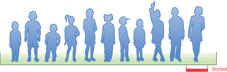
FIGURE 3-4 Bubble sort: the end of the first pass
After this first pass through all the players, you’ve made N−1 comparisons and somewhere between 0 and N−1 swaps, depending on the initial arrangement of the players. The player at the end of the line is sorted and won’t be moved again.
Now you go back and start another pass from the left end of the line. Again, you go toward the right, comparing and swapping when appropriate. This time, however, you can stop one player short of the end of the line, at position N−2, because you know the last position, at N−1, already contains the tallest player. This rule could be stated as:
When you reach the first sorted player, start over at the left end of the line.
You continue this process until all the players are in order. Describing this process is much harder than demonstrating it, so let’s watch its work in the SimpleSorting Visualization tool.
The SimpleSorting Visualization Tool
Start the SimpleSorting Visualization tool (run python3 SimpleSorting.py as described in Appendix A). This program shows an array of values and provides multiple ways of sorting and manipulating it. Figure 3-5 shows the initial display.
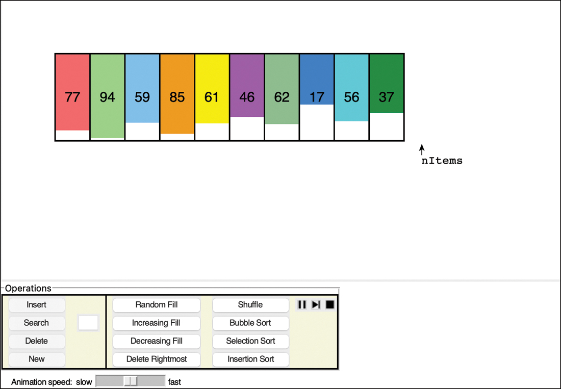
FIGURE 3-5 The SimpleSorting Visualization tool
The Insert, Search, Delete, New, Random Fill, and Delete Rightmost buttons function like those we saw in the Array Visualization tool used in Chapter 2. There are new buttons on the right relevant to sorting. Select the Bubble Sort button to start sorting the items. As with the other visualization tools, you can slow down or speed up the animation using the slider on the bottom. You can pause and resume playing the animation with the play, pause, and skip buttons (![]() ,
, ![]() ,
, ![]() ).
).
When the bubble sort begins, it adds two arrows labeled “inner” and “last” next to the array. These point to where the algorithm is doing its work. The inner arrow walks from the leftmost cell to the right, swapping item pairs when it finds a taller one to the left of a shorter one, just like the players on the team. It stops when it reaches the last arrow, which marks the first item that is in the final sorted order.
As each maximum item “bubbles” up to the far right, the last arrow moves to the left by one cell, to keep track of which items are sorted. When the last arrow moves all the way to the first cell on the left, the array is fully sorted. To run a new sort operation, select Shuffle, and then Bubble Sort again.
Try going through the bubble sort process using the step (![]() ) or play/pause (
) or play/pause (![]() /
/![]() ) buttons. At each step, think about what should happen next. Will a swap occur? How will the two arrows change?
) buttons. At each step, think about what should happen next. Will a swap occur? How will the two arrows change?
Try making a new array with many cells (30+) and filling it with random items. The cells will become too narrow to show the numbers of each item. The heights of the colored rectangles indicate their number, but it’s harder to see which one is taller when they are nearly equal in height. Can you still predict what will happen at each step?
The visualization tool also has buttons to fill empty cells with keys in increasing order and decreasing order. It’s interesting to see what happens when sorting algorithms encounter data that is already sorted or reverse sorted. You can also scramble the data with the Shuffle button to try running a new sort.
Note
The Stop (![]() ) button stops an animation and allows you to start other operations. The array contents, however, may be different than what they were at the start of the animation. There may be missing items or extra copies of items depending on when the operation was interrupted. In this way, the visualization mimics what happens in computer memory if something stops the execution.
) button stops an animation and allows you to start other operations. The array contents, however, may be different than what they were at the start of the animation. There may be missing items or extra copies of items depending on when the operation was interrupted. In this way, the visualization mimics what happens in computer memory if something stops the execution.
Python Code for a Bubble Sort
The bubble sort algorithm is pretty straightforward to explain, but we need to look at how to write the program. Listing 3-1 shows the bubbleSort() method of an Array class. It is almost the same as the Array class introduced in Chapter 2, and the full SortArray module is shown later in this chapter in Listing 3-4.
LISTING 3-1 The bubbleSort() method of the Array class
   def bubbleSort(self):                          # Sort comparing adjacent vals
      for last in range(self.__nItems-1, 0, -1):  # and bubble up
         for inner in range(last):                # inner loop goes up to last
            if self.__a[inner] > self.__a[inner+1]:  # If item less
               self.swap(inner, inner+1)          # than adjacent item, swap
In the Array class, each element of the array is assumed to be a simple value that can be compared with any of the other values for the purposes of ordering them. We reintroduce a key function to handle ordering records later.
The bubbleSort() method has two loops. The inner loop handles stepping through the array and swapping elements that are out of order. The outer loop handles the decreasing length of the unsorted part of the array. The outer loop sets the last variable to point initially at the last element of the array. That’s done by using Python’s range function to start at __nItems-1 and step down to 1 in increments of −1. The inner loop starts each time with the inner variable set to 0 and increments by 1 to reach last-1. The elements at indices greater than last are always completely sorted. After each pass of the inner loop, the last variable can be reduced by 1 because the maximum element between 0 and last bubbled up to the last position.
The inner loop body performs the test to compare the elements at the inner and inner+1 indices. If the value at inner is larger than the one to its right, you have to swap the two array elements (we’ll see how swap() works when we look at all the SortArray code in a later section).
Invariants
In many algorithms, there are conditions that remain unchanged as the algorithm proceeds. These conditions are called invariants. Recognizing invariants can be useful in understanding the algorithm. In certain situations, they may help in debugging; you can repeatedly check that the invariant is true, and signal an error if it isn’t.
In the bubbleSort() method, the invariant is that the array elements to the right of last are sorted. This remains true throughout the running of the algorithm. On the first pass, nothing has been sorted yet, and there are no items to the right of last because it starts on the rightmost element.
Efficiency of the Bubble Sort
If you use bubble sort on an array with 11 cells, the inner arrow makes 10 comparisons on the first pass, nine on the second, and so on, down to one comparison on the last pass. For 11 items, this is
10 + 9 + 8 + 7 + 6 + 5 + 4 + 3 + 2 + 1 = 55
In general, where N is the number of items in the array, there are N−1 comparisons on the first pass, N−2 on the second, and so on. The formula for the sum of such a series is
(N−1) + (N−2) + (N−3) + ... + 1 = N×(N−1)/2
N×(N−1)/2 is 55 (11×10/2) when N is 11.
Thus, the algorithm makes about N2/2 comparisons (ignoring the −1, which doesn’t make much difference, especially if N is large).
There are fewer swaps than there are comparisons because two bars are swapped only if they need to be. If the data is random, a swap is necessary about half the time, so there would be about N2/4 swaps. (In the worst case, with the initial data inversely sorted, a swap is necessary with every comparison.)
Both swaps and comparisons are proportional to N2. Because constants don’t count in Big O notation, you can ignore the 2 and the 4 in the divisor and say that the bubble sort runs in O(N2) time. This is slow, as you can verify by running the Bubble Sort in the SimpleSorting Visualization tool with arrays of 20+ cells.
Whenever you see one loop nested within another, such as those in the bubble sort and the other sorting algorithms in this chapter, you can suspect that an algorithm runs in O(N2) time. The outer loop executes N times, and the inner loop executes N (or perhaps N divided by some constant) times for each cycle of the outer loop. This means it’s doing something approximately N×N or N2 times.
Selection Sort
How can you improve the efficiency of the sorting operation? You know that O(N2) is pretty bad. Can you get to O(N) or maybe even O(log N)? We look next at a method called selection sort, which reduces the number of swaps. That could be significant when sorting large records by a key. Copying entire records rather than just integers could take much more time than comparing two keys. In Python as in other languages, the computer probably just copies pointers or references to record objects rather than the entire record, but it’s important to understand which operations are happening the most times.
Selection Sort on the Football Players
Let’s consider the football players again. In the selection sort, you don’t compare players standing next to each other, but you still can look at only two players and compare their heights. In this algorithm, you need to remember a certain player’s height—perhaps by using a measuring stick and writing the number in a notebook. A ball also comes in handy as a marker.
A Brief Description
What’s involved in the selection sort is making a pass through all the players and picking (or selecting, hence the name of the sort) the shortest one. This shortest player is then swapped with the player on the left end of the line, at position 0. Now the leftmost player is sorted and doesn’t need to be moved again. Notice that in this algorithm the sorted players accumulate on the left (lower indices), whereas in the bubble sort they accumulated on the right.
The next time you pass down the row of players, you start at position 1, and, finding the minimum, swap with position 1. This process continues until all the players are sorted.
A More Detailed Description
Let’s start at the left end of the line of players. Record the leftmost player’s height in your notebook and put a ball on the ground in front of this person. Then compare the height of the next player to the right with the height in your notebook. If this player is shorter, cross out the height of the first player and record the second player’s height instead. Also move the ball, placing it in front of this new “shortest” (for the time being) player. Continue down the row, comparing each player with the minimum. Change the minimum value in your notebook and move the ball whenever you find a shorter player. When you reach the end of the line, the ball will be in front of the shortest player. For example, the top of Figure 3-6 shows the ball being placed in front of the fourth player from the left.
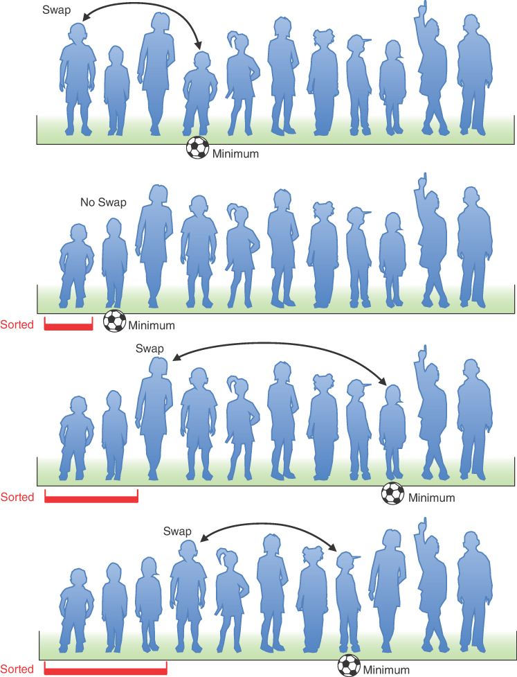
FIGURE 3-6 Selection sort on football players
Swap this shortest player with the player on the left end of the line. You’ve now sorted one player. You’ve made N−1 comparisons, but only one swap.
On the next pass, you do exactly the same thing, except that you can skip the player on the left because this player has already been sorted. Thus, the algorithm starts the second pass at position 1, instead of 0. In the case of Figure 3-6, this second pass finds the shortest player at position 1, so no swap is needed. With each succeeding pass, one more player is sorted and placed on the left, and one fewer player needs to be considered when finding the new minimum. The bottom of Figure 3-6 shows how this sort looks after the first three passes.
The Selection Sort in the SimpleSorting Visualization Tool
To see how the selection sort looks in action, try out the Selection Sort button in the SimpleSorting Visualization tool. Use the New and Random Fill buttons to create a new array of 11 randomly arranged items. When you select the Selection Sort button, it adds arrows to the display that look something like those shown in Figure 3-7. The arrow labeled “outer” starts on the left along with a second arrow labeled “min.” The “inner” arrow starts one cell to the right and marks where the first comparison happens.
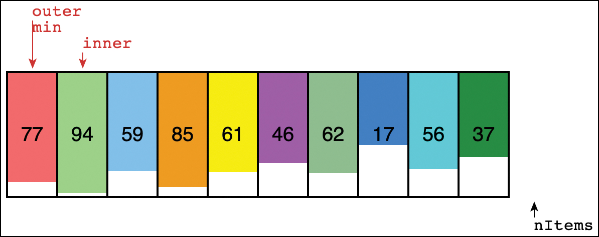
FIGURE 3-7 The start of a selection sort in the SimpleSorting Visualization tool
As inner moves right, each cell it points at is compared with the one at min. If the value at min is lower, then the min arrow is moved to where inner is, just as you moved the ball to lie in front of the shortest player.
When inner reaches the right end, the items at the outer and min arrows are swapped. That means that one more cell has been sorted, so outer can be moved one cell to the right. The next pass starts with min pointing to the new position of outer and inner one cell to their right.
The outer arrow marks the position of the first unsorted item. All items from outer to the right end are unsorted. Cells to the left of outer are fully sorted. The sorting continues until outer reaches the last cell on the right. At that point, the next possible comparison would have to be past the last cell, so the sorting must stop.
Python Code for Selection Sort
As with the bubble sort, implementing a selection sort requires two nested loops. The Python method is shown in Listing 3-2.
LISTING 3-2 The selectionSort() Method of the Array Class
   def selectionSort(self):                     # Sort by selecting min and
      for outer in range(self.__nItems-1):      # swapping min to leftmost
         min = outer                            # Assume min is leftmost
         for inner in range(outer+1, self.__nItems): # Hunt to right
            if self.__a[inner] < self.__a[min]: # If we find new min,
               min = inner                      # update the min index

         # __a[min] is smallest among __a[outer]...__a[__nItems-1]
         self.swap(outer, min)                  # Swap leftmost and min
The outer loop starts by setting the outer variable to point at the beginning of the array (index 0) and proceeds right toward higher indices. The minimum valued item is assumed to be the first one by setting min to be the same as outer. The inner loop, with loop variable inner, begins at outer+1 and likewise proceeds to the right.
At each new position of inner, the elements __a[inner] and __a[min] are compared. If __a[inner] is smaller, then min is given the value of inner. At the end of the inner loop, min points to the minimum value, and the array elements pointed to by outer and min are swapped.
Invariant
In the selectionSort() method, the array elements with indices less than outer are always sorted. This condition holds when outer reaches __nItems-1, which means all but one item are sorted. At that point, you could try to run the inner loop one more time, but it couldn’t change the min index from outer because there is only one item left in the unsorted range. After doing nothing in the inner loop, it would then swap the item at outer with itself—another do nothing operation—and then outer would be incremented to __nItems. Because that entire last pass does nothing, you can end when outer reaches __nItems-1.
Efficiency of the Selection Sort
The comparisons performed by the selection sort are N×(N−1)/2, the same as in the bubble sort. For 11 data items, this is 55 comparisons. That process requires exactly 10 swaps. The number of swaps is always N−1 because the outer loop does one for each iteration. That compares favorably with the approximately N2/4 swaps needed in bubble sort, which works out to about 30 for 11 items. With 100 items, the selection sort makes 4,950 comparisons and 99 swaps. For large values of N, the comparison times dominate, so you would have to say that the selection sort runs in O(N2) time, just as the bubble sort did. It is, however, unquestionably faster because there are O(N) instead of O(N2) swaps. Note that the number of swaps in bubble sort is dependent on the initial ordering of the array elements, so in some special cases, they could number fewer than those made by the selection sort.
Insertion Sort
In most cases, the insertion sort is the best of the elementary sorts described in this chapter. It still executes in O(N2) time, but it’s about twice as fast as the bubble sort and somewhat faster than the selection sort in normal situations. It’s also not too complex, although it’s slightly more involved than the bubble and selection sorts. It’s often used as the final stage of more sophisticated sorts, such as quicksort.
Insertion Sort on the Football Players
To begin the insertion sort, start with the football players lined up in random order. (They wanted to play a game, but clearly they’ve got to wait until the picture can be taken.) It’s easier to think about the insertion sort if you begin in the middle of the process, when part of the team is sorted.
Partial Sorting
You can use your handy ball to mark a place in the middle of the line. The players to the left of this marker are partially sorted. This means that they are sorted among themselves; each one is taller than the person to their left. The players, however, aren’t necessarily in their final positions because they may still need to be moved when previously unsorted players are inserted between them.
Note that partial sorting did not take place in the bubble sort and selection sort. In these algorithms, a group of data items was completely sorted into their final positions at any given time; in the insertion sort, one group of items is only partially sorted.
The Marked Player
The player where the marker ball is, whom we call the “marked” player, and all the players to the right are as yet unsorted. Figure 3-8 shows the process. At the top, the players are unsorted. The next row in the figure shows the situation three steps later. The marker ball is put in front of a player who has stepped forward.
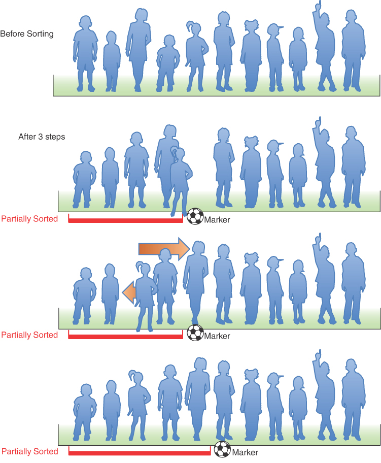
FIGURE 3-8 The insertion sort on football players
What you’re going to do is insert the marked player in the appropriate place in the (partially) sorted group. To do this, you need to shift some of the sorted players to the right to make room. To provide a space for this shift, the marked player is taken out of line. (In the program, this data item is stored in a temporary variable.) This step is shown in the second row of Figure 3-8.
Now you shift the sorted players to make room. The tallest sorted player moves into the marked player’s spot, the next-tallest player into the tallest player’s spot, and so on as shown by the arrows in the third row of the figure.
When does this shifting process stop? Imagine that you and the marked player are walking down the line to the left. At each position you shift another player to the right, but you also compare the marked player with the player about to be shifted. The shifting process stops when you’ve shifted the last player that’s taller than the marked player. The last shift opens up the space where the marked player, when inserted, will be in sorted order. This step is shown in the bottom row of Figure 3-8.
Now the partially sorted group is one player bigger, and the unsorted group is one player smaller. The marker ball is moved one space to the right, so it’s again in front of the leftmost unsorted player. This process is repeated until all the unsorted players have been inserted (hence the name insertion sort) into the appropriate place in the partially sorted group.
The Insertion Sort in the SimpleSorting Visualization Tool
Return to the SimpleSorting Visualization tool and create another 11-cell array of random values. Then select the Insertion Sort button to start the sorting process. As in the other sort operations, the algorithm puts up two arrows: one for the outer and one for the inner loops. The arrow labeled “outer” is the equivalent of the marker ball in sorting the players.
In the example shown in Figure 3-9, the outer arrow is pointing at the fifth cell in the array. It already copied item 61 to the temp variable below the array. It has also copied item 94 into the fifth cell and is starting to copy item 85 into the fourth. The four cells to the left of the outer arrow are partially sorted; the cells to its right are unsorted. Even while it decides where the marked player should go and there are extra copies of one of them, the left-hand cells remain partially sorted. This matches what happens in the computer memory when you copy the array item to a temporary variable.
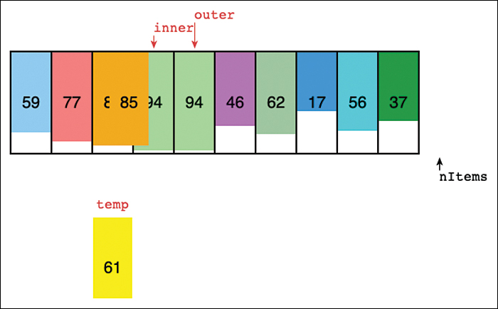
FIGURE 3-9 In the middle of an insertion sort in the SimpleSorting Visualization tool
The inner arrow starts at the same cell as the outer arrow and moves to the left, shifting items taller than the marked temp item to the right. In Figure 3-9, item 85 is being copied to where inner points because it is larger than item 61. After that copy is completed, inner moves one cell to the left and finds that item 77 needs to be moved too. On the next step for inner, it finds item 59 to its left. That item is smaller than 61, and the marked item is copied from temp back to the inner cell, where item 77 used to be.
Try creating a larger array filled with random values. Run the insertion sort and watch the updates to the arrows and items. Everything to the left of the outer arrow remains sorted by height. The inner arrow moves to the left, shifting items until it finds the right cell to place the item that was marked (copied from the outer cell).
Eventually, the outer arrow arrives at the right end of the array. The inner arrow moves to the left from that right edge and stops wherever it is appropriate to insert the last item. It might finish anywhere in the array. That’s a little different than the bubble and selection sorts where the outer and inner loop variables finish together.
Notice that, occasionally, the item copied from outer to temp is copied right back to where it started. That occurs when outer happens to point at an item larger than every item to its left. A similar thing happens in the selection sort when the outer arrow points at an item smaller than every item to its right; it ends up doing a swap with itself. Doing these extra data moves might seem inefficient, but adding tests for these conditions could add its own inefficiencies. An experiment at the end of the chapter asks you to explore when it might make sense to do so.
Python Code for Insertion Sort
Let’s now look at the insertionSort() method for the Array class as shown in Listing 3-3. You still need two loops, but the inner loop hunts for the insertion point using a while loop this time.
LISTING 3-3 The insertionSort() method of the Array class
   def insertionSort(self):                     # Sort by repeated inserts
      for outer in range(1, self.__nItems):     # Mark one element
         temp = self.__a[outer]                 # Store marked elem in temp
         inner = outer                          # Inner loop starts at mark
         while inner > 0 and temp < self.__a[inner-1]: # If marked
            self.__a[inner] = self.__a[inner-1] # elem smaller, then
            inner -= 1                          # shift elem to right
         self.__a[inner] = temp                 # Move marked elem to 'hole'
In the outer for loop, outer starts at 1 and moves right. It marks the leftmost unsorted array element. In the inner while loop, inner starts at outer and moves left to inner-1, until either temp is smaller than the array element there, or it can’t go left any further. Each pass through the while loop shifts another sorted item one space right.
Invariants in the Insertion Sort
The data items with smaller indices than outer are partially sorted. This is true even at the beginning when outer is 1 because the single item in cell 0 forms a one-element sequence that is always sorted. As items shift, there are multiple copies of one of them, but they all remain in partially sorted order.
Efficiency of the Insertion Sort
How many comparisons and copies does this algorithm require? On the first pass, it compares a maximum of one item. On the second pass, it’s a maximum of two items, and so on, up to a maximum of N−1 comparisons on the last pass. (We ignore the check for inner > 0 and count only the intra-element comparisons.) This adds up to
1 + 2 + 3 + … + N−1 = N×(N−1)/2
On each pass, however, the number of items actually compared before the insertion point is found is, on average, half of the partially sorted items, so you can divide by 2, which gives
N×(N−1)/4
The number of copies is approximately the same as the number of comparisons because it makes one copy for each comparison but the last. Copying one item is less time-consuming than a swap of two items, so for random data this algorithm runs twice as fast as the bubble sort and faster than the selection sort, on average.
In any case, like the other sort routines in this chapter, the insertion sort runs in O(N2) time for random data.
For data that is already sorted or almost sorted, the insertion sort does much better. When data is in order, the condition in the while loop is never true, so it becomes a simple statement in the outer loop, which executes N−1 times. In this case, the algorithm runs in O(N) time. If the data is almost sorted, the insertion sort runs in almost O(N) time, which makes it a simple and efficient way to order an array that is only slightly out of order.
For data arranged in inverse sorted order, however, every possible comparison and shift is carried out, so the insertion sort runs no faster than the bubble sort. Try some experiments with the SimpleSorting Visualization tool. Sort an 8+ element array with the selection sort and then try sorting the result with the selection sort again. Even though the second attempt doesn’t make any “real” swaps, it takes the same number of steps to go through the process. Then shuffle the array and sort it twice using the insertion sort. The second attempt at the insertion sort is significantly shorter because the inner loop ends after one comparison.
Python Code for Sorting Arrays
Now let’s combine the three sorting algorithms into a single object class to compare them. Starting from the Array class introduced in Chapter 2, we add the new methods for swapping and sorting plus the __str__() method for displaying the contents of arrays as a string and put them in a module called SortArray.py, as shown in Listing 3-4.
LISTING 3-4 The SortArray.py module
# Implement a sortable Array data structure

class Array(object):
   def __init__(self, initialSize):    # Constructor
      self.__a = [None] * initialSize  # The array stored as a list
      self.__nItems = 0                # No items in array initially

   def __len__(self):                  # Special def for len() func
      return self.__nItems             # Return number of items

   def get(self, n):                   # Return the value at index n
      if 0 <= n and n < self.__nItems: # Check if n is in bounds, and
         return self.__a[n]            # only return item if in bounds

   def set(self, n, value):            # Set the value at index n
      if 0 <= n and n < self.__nItems: # Check if n is in bounds, and
         self.__a[n] = value           # only set item if in bounds

   def swap(self, j, k):               # Swap the values at 2 indices
      if (0 <= j and j < self.__nItems and # Check if indices are in
          0 <= k and k < self.__nItems): # bounds, before processing
         self.__a[j], self.__a[k] = self.__a[k], self.__a[j]

   def insert(self, item):             # Insert item at end
        if self.__nItems >= len(self.__a):   # If array is full,
         raise Exception("Array overflow")      # raise exception
      self.__a[self.__nItems] = item   # Item goes at current end
      self.__nItems += 1               # Increment number of items

   def find(self, item):               # Find index for item
      for j in range(self.__nItems):   # Among current items
         if self.__a[j] == item:       # If found,
            return j                   # then return index to element
      return -1                        # Not found -> return -1

   def search(self, item):             # Search for item
      return self.get(self.find(item)) # and return item if found

   def delete(self, item):             # Delete first occurrence
      for j in range(self.__nItems):   # of an item
         if self.__a[j] == item:       # Found item
            self.__nItems -= 1         # One fewer at end
            for k in range(j, self.__nItems):  # Move items from
               self.__a[k] = self.__a[k+1]     # right over 1
            return True                # Return success flag

      return False     # Made it here, so couldn't find the item

   def traverse(self, function=print): # Traverse all items
      for j in range(self.__nItems):   # and apply a function
         function(self.__a[j])

   def __str__(self):                  # Special def for str() func
      ans = "["                        # Surround with square brackets
      for i in range(self.__nItems):   # Loop through items
         if len(ans) > 1:              # Except next to left bracket,
            ans += ", "                # separate items with comma
         ans += str(self.__a[i])       # Add string form of item
      ans += "]"                       # Close with right bracket
      return ans

   def bubbleSort(self):               # Sort comparing adjacent vals
      for last in range(self.__nItems-1, 0, -1):  # and bubble up
         for inner in range(last):     # inner loop goes up to last
            if self.__a[inner] > self.__a[inner+1]: # If elem less
               self.swap(inner, inner+1) # than adjacent value, swap

   def selectionSort(self):            # Sort by selecting min and
      for outer in range(self.__nItems-1): # swapping min to leftmost
         min = outer                   # Assume min is leftmost
         for inner in range(outer+1, self.__nItems): # Hunt to right
            if self.__a[inner] < self.__a[min]: # If we find new min,
               min = inner             # update the min index

         # __a[min] is smallest among __a[outer]...__a[__nItems-1]
         self.swap(outer, min)         # Swap leftmost and min

   def insertionSort(self):            # Sort by repeated inserts
      for outer in range(1, self.__nItems): # Mark one element
         temp = self.__a[outer]        # Store marked elem in temp
         inner = outer                 # Inner loop starts at mark
         while inner > 0 and temp < self.__a[inner-1]: # If marked
            self.__a[inner] = self.__a[inner-1] # elem smaller, then
            inner -= 1                 # shift elem to right
         self.__a[inner] = temp        # Move marked elem to 'hole'
The swap() method swaps the values in two cells of the array. It ensures that swaps happen only with items that have been inserted in the array and not with allocated but uninitialized cells. Those tests may not be necessary with the sorting methods in this module that already ensure proper indices, but they are a good idea for a general-purpose routine.
We use a separate client program, SortArrayClient.py, to test this new module and compare the performance of the different sorting methods. This program uses some other Python modules and features to help in this process and is shown in Listing 3-5.
LISTING 3-5 The SortArrayClient.py program
from SortArray import *
import random
import timeit

def initArray(size=100, maxValue=100, seed=3.14159):
    """Create an Array of the specified size with a fixed sequence of
       'random' elements"""
    arr = Array(size)                          # Create the Array object
    random.seed(seed)                          # Set random number generator
    for i in range(size):                      # to known state, then loop
        arr.insert(random.randrange(maxValue)) # Insert random numbers
    return arr                                 # Return the filled Array

arr = initArray()
print("Array containing", len(arr), "items:
", arr)

for test in ['initArray().bubbleSort()',
             'initArray().selectionSort()',
             'initArray().insertionSort()']:
    elapsed = timeit.timeit(test, number=100, globals=globals())
    print(test, "took", elapsed, "seconds", flush=True)

arr.insertionSort()
print('Sorted array contains:
', arr)
The SortArrayClient.py program starts by importing the SortArray module to test the sorting methods, and the random and timeit modules to assist. The random module provides pseudo-random number generators that can be used to make test data. The timeit module provides a convenient way to measure the execution times of Python code.
The test program first defines a function, initArray(), that generates an unsorted array for testing. Right after the parameter list, it has a documentation string that helps explain its purpose, creating arrays of a fixed size filled with a sequence of random numbers. Because we’d like to test the different sort operations on the exact same sequence of elements, we want initArray() to return a fresh copy of the same array every time it runs, but conforming to the parameters it is given. The function first creates an Array of the desired size. Next, it initializes the random module to a known state by setting the seed value. This means that pseudo-random functions produce the same sequence of numbers when called in the same order.
Inside the following for loop, the random.randrange(maxValue) function generates integers in the range [0, maxValue) that are inserted into the array (the math notation [a, b) represents a range of numbers that includes a but excludes b). Then the filled array is returned.
The test program uses the initArray() function to generate an array that is stored in the arr variable. After printing the initial contents of arr, a for loop is used to step through the three sort operations to be timed. The loop variable, test, is bound to a string on each pass of the loop. The string has the Python expression whose execution time is to be measured. Inside the loop body, the timeit.timeit() function call measures the elapsed time of running the test expression. It runs the expression a designated number of times and returns the total elapsed time in seconds. Running it many times helps deal with the variations in running times due to other operations happening on the computer executing the Python interpreter. The last argument to timeit.timeit() is globals, which is needed so that the interpreter has all the definitions that have been loaded so far, including SortArray and initArray. The interpreter uses those definitions when evaluating the Python expression in the test variable.
The result of timeit.timeit() is stored in the elapsed variable and then printed out with flush=True so that it doesn’t wait until the output buffer is full or input needs to be read before printing. After all three test times are printed, it performs one more sort on the original arr array and prints its contents. The results look like this:
$ python3 SortArrayClient.py
Array containing 100 items:
 [77, 94, 59, 85, 61, 46, 62, 17, 56, 37, 18, 45, 76, 21, 91, 7, 96, 50, 31, 69, 80,
69, 56, 60, 26, 25, 1, 2, 67, 46, 99, 57, 32, 26, 98, 51, 77, 34, 20, 81, 22, 40,
28, 23, 69, 39, 23, 6, 46, 1, 96, 51, 71, 61, 2, 34, 1, 55, 78, 91, 69, 23, 2, 8,
3, 78, 31, 25, 26, 73, 28, 88, 88, 38, 22, 97, 9, 18, 18, 66, 47, 16, 82, 9, 56, 45,
15, 76, 85, 52, 86, 5, 28, 67, 34, 20, 6, 33, 83, 68]
initArray().bubbleSort() took 0.25465869531035423 seconds
initArray().selectionSort() took 0.11350362841039896 seconds
initArray().insertionSort() took 0.12348053976893425 seconds
Sorted array contains:
 [1, 1, 1, 2, 2, 2, 3, 5, 6, 6, 7, 8, 9, 9, 15, 16, 17, 18, 18, 18, 20, 20, 21, 22,
22, 23, 23, 23, 25, 25, 26, 26, 26, 28, 28, 28, 31, 31, 32, 33, 34, 34, 34, 37, 38,
39, 40, 45, 45, 46, 46, 46, 47, 50, 51, 51, 52, 55, 56, 56, 56, 57, 59, 60, 61, 61,
62, 66, 67, 67, 68, 69, 69, 69, 69, 71, 73, 76, 76, 77, 77, 78, 78, 80, 81, 82, 83,
85, 85, 86, 88, 88, 91, 91, 94, 96, 96, 97, 98, 99]
Looking at the output, you can see that the randrange() function provided a broad variety of values for the array in a random order. The results of the timing of the sort tests show the bubble sort taking at least twice as much time as the selection and insertion sorts do. The final sorted version of the array confirms that sorting works and shows that there are many duplicate elements in the array.
Stability
Sometimes it matters what happens to data items that have equal keys when sorting. The SortArrayClient.py test stored only integers in the array, and equal integers are pretty much indistinguishable. If the array contained complex records, however, it could be very important how records with the same key are sorted. For example, you may have employee records arranged alphabetically by family names. (That is, the family names were used as key values in the sort.) Let’s say you want to sort the data by postal code too, but you want all the items with the same postal code to continue to be sorted by family names. This is called a secondary sort key. You want the sorting algorithm to shift only what needs to be sorted by the current key and leave everything else in its order after previous sorts using other keys. Some sorting algorithms retain this secondary ordering; they’re said to be stable. Stable sorting methods also minimize the number of swaps or copy operations.
Some of the algorithms in this chapter are stable. We have included an exercise at the end of the chapter for you to decide which ones are. The answer is not obvious from the output of their test programs, especially on simple integers. You need to review the algorithms to see that swaps and copies only happen on items that need to be moved to be in the right position for the final order. They should also move items with equal keys the minimum number of array cells necessary so that they remain in the same relative order in the final arrangement.
Comparing the Simple Sorts
There’s probably no point in using the bubble sort, unless you don’t have your algorithm book handy. The bubble sort is so simple that you can write it from memory. Even so, it’s practical only if the amount of data is small. (For a discussion of what “small” means and what trade-offs such decisions entail, see Chapter 16, “What to Use and Why.”)
Table 3-1 summarizes the time efficiency of each of the sorting methods. We looked at what the algorithms would do when presented with elements whose keys are in random order to determine what they would do in the average case. We also considered what would happen in the worst case when the keys were in some order that would maximize the number of operations. The table includes both the Big O notation followed by the detailed value in square brackets [ ]. The Big O notation is what matters most; it gives the broad classification of the algorithms and tells what will happen for very large N. Typically, we are most interested in the average case behavior because we cannot anticipate what data they will encounter, but sometimes the worst case is the driving factor. For example, if the sort must be able to complete within a specific amount of time for a particular size of data, we can use the best of the worst-case values to choose the algorithm that will guarantee that completion time.
Table 3-1 Time Order of the Sort Methods
Algorithm | Comparisons | Swaps or Copies | ||
|---|---|---|---|---|
Average case | Worst case | Average case | Worst case | |
Bubble sort | O(N2) [N2/2] | O(N2) [N2/2] | O(N2) [N2/4] | O(N2) [N2/2] |
Selection sort | O(N2) [N2/2] | O(N2) [N2/2] | O(N) [N−1] | O(N) [N−1] |
Insertion sort | O(N2) [N2/4] | O(N2) [N2/2] | O(N2) [N2/4] | O(N2) [N2/2] |
The detailed values shown in the table can be somewhat useful in narrow circumstances. For example, the relative number of comparisons in the average case between the bubble sort and the insertion sort corresponds well with the relative time measurements in the test program. That would also predict that the selection sort average case should be closer to the bubble sort, but the one measurement above doesn’t agree with that. Perhaps that means that the swaps or copies were a bigger factor on running time with N around 100 on the test platform.
Overall, the selection sort minimizes the number of swaps, but the number of comparisons is still high. This sort might be useful when the amount of data is small and swapping data items is very time-consuming relative to comparing them. In real-world scenarios, there can be situations where keeping the swaps to a minimum is more important than the number of comparisons. For example, in moving patients between hospital rooms (in response to some other disaster), it could be critical to displace as few patients as possible.
The insertion sort is the most versatile of the three sorting methods and is the best bet in most situations, assuming the amount of data is small, or the data is almost sorted. For larger amounts of data, quicksort and Timsort are generally considered the fastest approach; we examine them in Chapter 7.
We’ve compared the sorting algorithms in terms of speed. Another consideration for any algorithm is how much memory space it needs. All three of the algorithms in this chapter carry out their sort in place, meaning that they use the input array as the output array and very little extra memory is required. All the sorts require an extra variable to store an item temporarily while it’s being swapped or marked. Because that item can be quite large, you need to consider it, but the local variables for indices into the array are typically ignored.
Summary
 The sorting algorithms in this chapter all assume an array as a data storage structure.
- Sorting involves comparing the keys of data items in the array and moving the items (usually references to the items) around until they’re in sorted order.
- All the algorithms in this chapter execute in O(N2) time. Nevertheless, some can be substantially faster than others.
- An invariant is a condition that remains unchanged while an algorithm runs.
- The bubble sort is the least efficient but the simplest sort.
- The insertion sort is the most commonly used of the O(N2) sorts described in this chapter.
- The selection sort performs O(N2) comparisons and only O(N) swaps, which can be important when swap time is much more significant than comparison time.
- A sort is stable if the order of elements with the same key is retained.
- None of the sorts in this chapter require more than a single temporary record variable, in addition to the original array.
Questions
These questions are intended as a self-test for readers. Answers may be found in Appendix C.
1. Computer sorting algorithms are more limited than humans in that
a. the amount of data that computers can sort is much less than what humans can.
b. humans can invent new sorting algorithms, whereas computers cannot.
c. humans know what to sort, whereas computers need to be told.
d. computers can compare only two things at a time, whereas humans can compare small groups.
2. The two basic operations in simplesorting are _________ items and _________ them (or sometimes _________ them).
3. True or False: The bubble sort always ends up comparing every possible pair of items in the initial array.
4. The bubble sort algorithm alternates between
a. comparing and swapping.
b. moving and copying.
c. moving and comparing.
d. copying and comparing.
5. True or False: If there are N items, the bubble sort makes exactly N×N comparisons.
6. In the selection sort,
a. the largest keys accumulate on the left (low indices).
b. a minimum key is repeatedly discovered.
c. a number of items must be shifted to insert each item in its correctly sorted position.
d. the sorted items accumulate on the right.
7. True or False: If, on a particular computing platform, swaps take much longer than comparisons, the selection sort is about twice as fast as the bubble sort for all values of N.
8. Ignoring the details of where the computer stores each piece of data, what is a reasonable assumption about the ratio of the amounts of time taken for a copy operation versus a swap operation?
9. What is the invariant in the selection sort?
10. In the insertion sort, the “marked player” described in the text corresponds to which variable in the insertionSort() method?
a. inner
b. outer
c. temp
d. __a[outer]
11. In the insertion sort, the “partially sorted” group members are
a. the items that are already sorted but still need to be moved as a block.
b. the items that are in their final block position but may still need to be sorted.
c. only partially sorted in order by their keys.
d. the items that are sorted among themselves, but items outside the group may need to be inserted in the group.
12. Shifting a group of items left or right requires repeated __________.
13. In the insertion sort, after an item is inserted in the partially sorted group, it
a. is never moved again.
b. is never shifted to the left.
c. is often moved out of this group.
d. finds that its group is steadily shrinking.
14. The invariant in the insertion sort is that ________.
15. Stability might refer to
a. items with secondary keys being excluded from a sort.
b. keeping cities sorted by increasing population within each state, in a sort by state.
c. keeping the same given names matched with the same family names.
d. items keeping the same order of secondary keys without regard to primary keys.
Experiments
Carrying out these experiments will help to provide insights into the topics covered in the chapter. No programming is involved.
3-A The “Stability” section explains that stable sorting algorithms don’t change the relative position within the array of items having equal-valued keys. For example, when you’re sorting an array containing tuples by their first element such as
(elm, 1), (asp, 1), (elm, 2), (oak, 1)
the algorithm always produces
(asp, 1), (elm, 1), (elm, 2), (oak, 1)
and never
(asp, 1), (elm, 2), (elm, 1), (oak, 1)
Review each of the simplesorting algorithms in this chapter and determine if they are always stable.
Determining whether a sorting algorithm is stable or not can be difficult. Try walking through some sample inputs that include some equal-valued keys to see when those items are moved. If you can think of even one example where two items with equal keys are reordered from their original relative order, then you have proven that the algorithm is unstable. If you can’t think of an example where equal-valued keys are moved out of order, then the algorithm might be stable. To be sure, you need to provide more proof. That’s usually done by finding invariant conditions about a partial sequence of items as the algorithm progresses. For example, if you can show that the output array after index i contains only items in stable order, that condition stays valid at iteration j if it held in iteration j − 1, and that i always ends at index 0, then the algorithm must be stable.
Note that if you get stuck, we provide an answer for this exercise in Appendix C.
3-B Sometimes the items in an array might have just a few distinct keys with many copies. That creates a situation where there are many duplicates of the same key. Use the SimpleSorting Visualization tool to create an array with 15 cells and filled with only two distinct values, say 10 and 90. Try shuffling and sorting that kind of array with the three sorting algorithms. Do any of them show advantages or disadvantages over the others for this kind of data?
3-C In the selectionSort() method shown in Listing 3-2, the inner loop makes a swap on every pass. It doesn’t need to swap them if the value of the min and outer indices are the same. Would it make sense to add an additional comparison of those indices and perform the swap only if they are different? If so, under what conditions would that improve the performance? If not, why not?
Programming Projects
Writing programs to solve the Programming Projects helps to solidify your understanding of the material and demonstrates how the chapter’s concepts are applied. (As noted in the Introduction, qualified instructors may obtain completed solutions to the Programming Projects on the publisher’s website.)
3.1 In the bubbleSort() method (Listing 3-1) and the Visualization tool, the inner index always goes from left to right, finding the largest item and carrying it out on the right. Modify the bubbleSort() method so that it’s bidirectional. This means the inner index will first carry the largest item from left to right as before, but when it reaches last, it will reverse and carry the smallest item from right to left. You need two outer indexes, one on the right (the old last) and another on the left.
3.2 Add a method called median() to the Array class in the SortArray.py module (Listing 3-4). This method should return the median value in the array. (Recall that in a group of numbers, half are larger than the median and half are smaller.) Do it the easy way.
3.3 Add a method called deduplicate() to the Array class in the SortArray.py module (Listing 3-4) that removes duplicates from a previously sorted array without disrupting the order. You can use any of the sort methods in your test program to sort the data. You can imagine schemes in which all the items from the place where a duplicate was discovered to the end of the array would be shifted down one space every time a duplicate was discovered, but this would lead to slow O(N2) time, at least when there were a lot of duplicates. In your algorithm, make sure no item is moved more than once, no matter how many duplicates there are. This will give you an algorithm with O(N) time.
3.4 Another simple sort is the odd-even sort. The idea is to repeatedly make two passes through the array. On the first pass, you look at all the pairs of items, a[j] and a[j + 1], where j is odd (j = 1, 3, 5, …). If their key values are out of order, you swap them. On the second pass, you do the same for all the even values (j = 0, 2, 4, …). You do these two passes repeatedly until the array is sorted. Add an oddEvenSort() method to the Array class in the SortArray.py module (Listing 3-4). Perform the outer loop until no swaps occur to see how many passes are needed; one pass includes both odd-pair and even-pair swapping. Make sure it works for varying amounts of data and on good and bad initial orderings. After testing how many passes are needed before no more swaps occur, determine the maximum number of passes of the outer loop based on the length of the input array.
The odd-even sort is actually useful in a multiprocessing environment, where a separate processor can operate on each odd pair simultaneously and then on each even pair. Because the odd pairs are independent of each other, each pair can be checked—and swapped, if necessary—by a different processor. This makes for a very fast sort.
3.5 Modify the insertionSort() method in SortArray.py (Listing 3-4) so that it counts the number of copies and the number of item comparisons it makes during a sort and displays the totals. You need to look at the loop condition in the inner while loop and carefully count item comparisons. Use this program to measure the number of copies and comparisons for different amounts of inversely sorted data. Do the results verify O(N2) efficiency? Do the same for almost-sorted data (only a few items out of place). What can you deduce about the efficiency of this algorithm for almost-sorted data?
3.6 Here’s an interesting way to remove items with duplicate keys from an array. The insertion sort uses a loop-within-a-loop algorithm that compares every item in the array with the partially sorted items so far. One way to remove items with duplicate keys would be to modify the algorithm in the Array class in the SortArray.py module (Listing 3-4) so that it removes the duplicates as it sorts. Here’s one approach: When a duplicate key is found, instead of copying the duplicate back into the array cell at its sorted position, change the key for the marked item to be a special value that is treated as lower than any other possible key. With that low key value, it is automatically moved into place at the beginning of the array. By keeping track of how many duplicates are found, you know the end of duplicates and beginning of the remaining elements in the array. When the outer loop ends, the algorithm would have to make one more pass to shift the unique keys into the cells occupied by the duplicates. Write an insertionSortAndDedupe() method that performs this operation. Make sure to test that it works with all different kinds of input array data.