
Chapter 7
Advanced Sorting
In This Chapter
We started discussing sorting in the aptly titled Chapter 3, “Simple Sorting.” The sorts described there—the bubble, selection, and insertion sorts—are easy to implement but rather slow. In Chapter 6, “Recursion,” we described the mergesort. It runs much faster than the simple sorts but requires twice as much space as the original array; this is often a serious drawback.
This chapter covers two advanced approaches to sorting in detail: Shellsort and quicksort. These sorts both operate much faster than the simple sorts: the Shellsort in about O(N×(log N)2) time, and quicksort in O(N×log N) time. Neither of these sorts requires a large amount of extra space, as mergesort does. The Shellsort is almost as easy to implement as mergesort although quicksort is the fastest of all the general-purpose sorts that don’t require a lot of memory.
We examine the Shellsort first. Quicksort is based on the idea of partitioning, so we examine that separately, before examining quicksort itself. We conclude the chapter with short descriptions of radix sort and Timsort, which are quite different approaches to fast sorting.
Shellsort
The Shellsort is named for Donald L. Shell, the computer scientist who discovered it in 1959. It’s based on the insertion sort but adds a new feature that dramatically improves the insertion sort’s performance.
The Shellsort is good for medium-sized arrays, depending on the particular implementation. It’s not quite as fast as quicksort and other O(N×log N) sorts, so it’s not optimum for very large collections. Shellsort, however, is much faster than the O(N2) sorts like the selection sort and the insertion sort, and it’s very easy to implement. The code is short and simple.
Shellsort’s worst-case performance is not significantly worse than its average performance. (Later in this chapter we look into that the worst-case performance for quicksort, which can be much worse unless precautions are taken.) Some experts (see Sedgewick in Appendix B, “Further Reading”) recommend starting with a Shellsort for almost any sorting project and changing to a more advanced sort, like quicksort, only if Shellsort proves too slow in practice.
Insertion Sort: Too Many Copies
Because Shellsort is based on the insertion sort, you might want to review the “Insertion Sort” section in Chapter 3. Recall that partway through the insertion sort the items to the left of a marker are partially sorted (sorted among themselves), and the items to the right are not. The algorithm removes the item at the marker and stores it in a temporary variable. Then, beginning with the item to the left of the newly vacated cell, it shifts the sorted items right one cell at a time, until the item in the temporary variable can be reinserted in sorted order.
Here’s the problem with the insertion sort. Suppose a small item is on the far right, where the large items should be. To move this small item to its proper place on the left, all the intervening items (between the place where it is and where it should be) must be shifted one space right. This step takes close to N copies, just for one item. Not all the items must be moved a full N spaces, but the average item must be moved N/2 spaces, which means the full process takes N times N/2 shifts for a total of N2/2 copies. Thus, the performance of insertion sort is O(N2).
This performance could be improved if you could somehow move a smaller item many spaces to the left without shifting all the intermediate items individually.
N-Sorting
The Shellsort achieves these large shifts by insertion-sorting widely spaced elements. After they are sorted, Shellsort sorts somewhat less widely spaced elements, and so on. The spacing between elements for these sorts is called the increment and is traditionally represented by the letter h. Figure 7-1 shows the first step in the process of sorting a 10-element peg board (array) with an increment of 4. Here the elements at indices 0, 4, and 8 are sorted.

FIGURE 7-1 4-sorting at 0, 4, and 8
After the pegs at 0, 4, and 8 are sorted, the algorithm shifts over one cell and sorts the pegs at locations 1, 5, and 9. This process continues until all the pegs have been 4-sorted, which means that all items spaced four cells apart are sorted among themselves. Figure 7-2 illustrates the process with different panels showing the state after each subset is sorted.
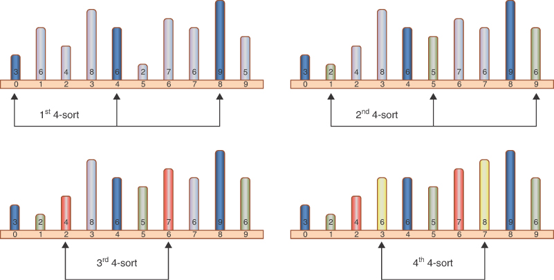
FIGURE 7-2 A complete 4-sort
After the complete 4-sort, the array can be thought of as comprising four subarrays with heights: [3,6,9], [2,5,6], [4,7], and [6,8], each of which is completely sorted. These subarrays are interleaved at locations [0,4,8], [1,5,9], [2,6], and [3,7] respectively—as shown by the colors of the pegs in the figure—but otherwise independent.
What has been gained? Well, the h-sorts have reduced the size of the number of items to be sorted in a single group. Instead of sorting N items, you’ve sorted N/h items h times. Because the insertion sort is an algorithm that is O(N2), that makes h-sorting O((N/h)2×h) = O(N2/h), so that’s an improvement. If h were big, say N/2, then the overall complexity would get down to O(N). Of course, the array isn’t fully sorted yet, but note that the items are closer to their final positions.
In the example of sorting 10 items in Figure 7-2, at the end of the 4-sort, no item is more than three cells from where it would be if the array were completely sorted. This is what is meant by an array being “almost” sorted and is the secret of the Shellsort. By creating interleaved, internally sorted sets of items using “inexpensive” h-sorts, you minimize the amount of work that must be done to complete the sort.
Now, as we noted in Chapter 3, the insertion sort is very efficient when operating on an array that’s almost sorted. In fact, for an already-sorted array, it’s O(N). If it needs to move items only one or two cells to sort the array, it can operate in almost O(N) time. Thus, after the array has been 4-sorted, you can 1-sort it using the ordinary insertion sort. The combination of the 4-sort and the 1-sort is much faster than simply applying the ordinary insertion sort without the preliminary 4-sort.
Diminishing Gaps
We’ve shown an initial interval—or gap—of four cells for sorting a 10-cell array. For larger arrays, the interval should start out much larger. The interval is then repeatedly reduced until it becomes 1.
For instance, an array of 1,000 items might be 364-sorted, then 121-sorted, then 40-sorted, then 13-sorted, then 4-sorted, and finally 1-sorted. The sequence of numbers used to generate the intervals (in this example, 364, 121, 40, 13, 4, 1) is called the interval sequence or gap sequence. The particular interval sequence shown here, attributed to Knuth (see Appendix B), is a popular one. In reversed form, starting from 1, it’s generated by the expression
hi = 3×hi–1 + 1
where the initial value of h0 is 1. Table 7-1 shows how this formula generates the sequence.
Table 7-1 Knuth's Interval Sequence
i | hi | 3×hi + 1 | (hi – 1) / 3 |
|---|---|---|---|
0 | 1 | 4 | |
1 | 4 | 13 | 1 |
2 | 13 | 40 | 4 |
3 | 40 | 121 | 13 |
4 | 121 | 364 | 40 |
5 | 364 | 1,093 | 121 |
6 | 1,093 | 3,280 | 364 |
There are other approaches to generating the interval sequence; we return to this issue later. First, let’s explore how the Shellsort works using Knuth’s sequence.
In the sorting algorithm, the sequence-generating formula is first used in a short loop to figure out the initial gap. A value of 1 is used for the first value of h, and the hi = 3×hi–1 + 1 formula is applied to generate the sequence 1, 4, 13, 40, 121, 364, and so on. This process ends when the gap is larger than the array. For a 1,000-element array, the seventh number in the sequence, 1,093, is too large. Thus, Shellsort begin the sorting process with the sixth-largest number, creating a 364-sort. Then, each time through the outer loop of the sorting routine, it reduces the interval using the inverse of the formula previously given
hi–1 = (hi – 1) / 3
This sequence is shown in the last column of Table 7-1. This inverse formula generates the reverse sequence 364, 121, 40, 13, 4, 1. Starting with 364, each of these numbers is used to h-sort the array. When the array has been 1-sorted, the algorithm is done.
The AdvancedSorting Visualization Tool
You can use the AdvancedSorting Visualization tool to see how Shellsort works. Figure 7-3 shows the tool as the Shellsort begins and determines what h value to use.

FIGURE 7-3 The AdvancedSorting Visualization tool
Like the Simple Sorting Visualization tool introduced in Chapter 3, this tool provides the common operations for inserting, searching, and deleting single items. It also allows you to create new arrays of empty cells and fill empty cells with random keys or keys that increase or decrease.
As you watch the Shellsort, you’ll notice that the explanation we gave in the preceding discussion is slightly simplified. The sequence of indices processed by the 4-sort is not actually [0, 4, 8], [1, 5, 9], [2, 6], and [3, 7]. Instead, the first two elements of the first group of three are sorted, then the first two elements of the second group, and so on. After the first two elements of all the groups are sorted, the algorithm returns and sorts the last element of the three-element groups. This is what happens in the insertion sort; the actual sequence is [0, 4], [1, 5], [2, 6], [3, 7], [0, 4, 8], [1, 5, 9].
It might seem more obvious for the algorithm to 4-sort each complete subarray first, that is, [0, 4], [0, 4, 8], [1, 5], [1, 5, 9], [2, 6], [3, 7], but the algorithm handles the array indices more efficiently using the first scheme.
The Shellsort is actually not very efficient with only 10 items, making almost as many swaps and comparisons as the insertion sort. With larger arrays, however, the improvement becomes significant.
Figure 7-4 shows the AdvancedSorting Visualization tool starting with a 90-cell array of inversely sorted bars. (Creating such a large array in the visualization tool requires making the window much wider before using the New button.) The Decreasing Fill button fills the empty cells with the values in the top row of the figure. The second row shows the array after it has been completely 40-sorted. On the left, the outer and inner indices are set to their values for the beginning of the 13-sort. The first two cells to be compared in the 13-sort are lowered from their normal position to show what cells are being checked. The third row shows the beginning of the 4-sort.

FIGURE 7-4 After the 40-sort and 13-sort in a 90-cell array
With each new value of h, the array becomes more nearly sorted. The groups of 40 are clear in the second row of Figure 7-4. The first 10 items are the shortest of the whole array. They came from the top 10 items of the initial array during the 40-sort. The next groups of 40 cells have runs of 30 and 10 decreasing keys each. The runs of 30 came from the 40-sorts on subarrays like indices [11, 51]. They keep the overall trend of decreasing keys, but each subarray is now in increasing order. When you get to the 4-sort starting in the last row of the figure, the overall trend now looks to be generally increasing. Every item is now within 13 cells of its final position. After the 4-sort, every item will be within four cells of its final position.
Why is the Shellsort so much faster than the insertion sort, on which it’s based? As mentioned previously, when h is large, the number of items per pass is small, and items move long distances. This sort is very efficient. As h grows smaller, the number of items per pass increases, but the items are already closer to their final sorted positions, which is more efficient for the insertion sort. It’s the combination of these trends that makes the Shellsort so effective.
Notice that later sorts (small values of h) don’t undo the work of earlier sorts (large values of h). An array that has been 40-sorted remains 40-sorted after a 13-sort, for example. If this wasn’t so, the Shellsort couldn’t work.
Python Code for the Shellsort
The Python code for the Shellsort is scarcely more complicated than for the insertion sort shown in Chapter 3. The key difference, of course, is the addition of the h interval and ensuring that the program takes steps of h elements instead of 1. Here, we add a ShellSort() method to the Array class (that was defined in the SortArray.py module) and put it into the ShellSort.py module shown in Listing 7-1.
The first part sets the initial h value. Starting at 1, it follows Knuth’s sequence to increment h, as long as it stays below about a third of the array size. A variable, nShifts, has been added to count the number of shift operations performed during the sorting. It’s not really necessary but helps to illustrate and instrument the actual complexity on specific arrays.
The main loop iterates over the h value, decreasing it through Knuth’s sequence until it gets below 1. The revised insertion sort algorithm appears inside the main loop. This time, outer starts at h. That is the index of the first cell that is not yet sorted (remember every cell below outer—stepping in increments of h—is already sorted). The value at outer is stored in temp as the marked item. The inner loop then sets its index, inner, to start at outer and work backward to lower indices stepping by h. After the inner loop finds that inner has reached the last possible index for this h-sort or the marked item, temp, is bigger than or equal to what is in the cell at inner - h, it stops. As the inner loop steps backward, it shifts the contents of the cells it passes (where the marked item is less than the value at inner – h). It increments the nShifts counter accordingly and does so once more at the end of the inner loop, if moving the marked item from temp back to the array is warranted.
LISTING 7-1 The ShellSort.py Module
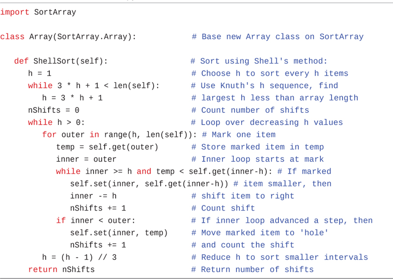
import SortArray

class Array(SortArray.Array):            # Base new Array class on SortArray

   def ShellSort(self):                  # Sort using Shell's method:
      h = 1                              # Choose h to sort every h items
      while 3 * h + 1 < len(self):       # Use Knuth's h sequence, find
         h = 3 * h + 1                   # largest h less than array length
      nShifts = 0                        # Count number of shifts
      while h > 0:                       # Loop over decreasing h values
         for outer in range(h, len(self)): # Mark one item
            temp = self.get(outer)       # Store marked item in temp
            inner = outer                # Inner loop starts at mark
            while inner >= h and temp < self.get(inner-h): # If marked
               self.set(inner, self.get(inner-h)) # item smaller, then
               inner -= h                # shift item to right
               nShifts += 1              # Count shift
            if inner < outer:            # If inner loop advanced a step, then
               self.set(inner, temp)     # Move marked item to 'hole'
               nShifts += 1              # and count the shift
         h = (h - 1) // 3                # Reduce h to sort smaller intervals
      return nShifts                     # Return number of shifts
After completing the first pass, the outer variable is incremented by 1 to move on to the next h-sort group. In terms of the first example, this means going from the [0, 4] subsequence to the [1, 5] subsequence. Incrementing outer by 1 all the way up to the length of the array eventually covers the longer subsequences like [0, 4, 8], [1, 5, 9], and so on. The outermost while loop decreases h following Knuth’s formula to perform the h-sort on smaller increments.
The Shellsort algorithm, although it’s implemented in just a few lines, is not simple to follow. Here’s a sample output from running it with some print statements:
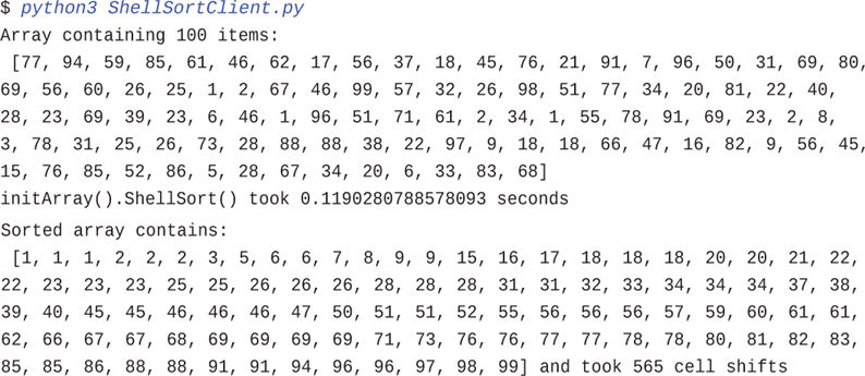
$ python3 ShellSortClient.py
Array containing 100 items:
 [77, 94, 59, 85, 61, 46, 62, 17, 56, 37, 18, 45, 76, 21, 91, 7, 96, 50, 31, 69, 80,
69, 56, 60, 26, 25, 1, 2, 67, 46, 99, 57, 32, 26, 98, 51, 77, 34, 20, 81, 22, 40,
28, 23, 69, 39, 23, 6, 46, 1, 96, 51, 71, 61, 2, 34, 1, 55, 78, 91, 69, 23, 2, 8,
3, 78, 31, 25, 26, 73, 28, 88, 88, 38, 22, 97, 9, 18, 18, 66, 47, 16, 82, 9, 56, 45,
15, 76, 85, 52, 86, 5, 28, 67, 34, 20, 6, 33, 83, 68]
initArray().ShellSort() took 0.1190280788578093 seconds
Sorted array contains:
 [1, 1, 1, 2, 2, 2, 3, 5, 6, 6, 7, 8, 9, 9, 15, 16, 17, 18, 18, 18, 20, 20, 21, 22,
22, 23, 23, 23, 25, 25, 26, 26, 26, 28, 28, 28, 31, 31, 32, 33, 34, 34, 34, 37, 38,
39, 40, 45, 45, 46, 46, 46, 47, 50, 51, 51, 52, 55, 56, 56, 56, 57, 59, 60, 61, 61,
62, 66, 67, 67, 68, 69, 69, 69, 69, 71, 73, 76, 76, 77, 77, 78, 78, 80, 81, 82, 83,
85, 85, 86, 88, 88, 91, 91, 94, 96, 96, 97, 98, 99] and took 565 cell shifts
Now that you’ve looked at the code, go back to the AdvancedSorting Visualization tool and follow the details of its operation, stepping through the process of Shellsorting a 10-item array. The visualization makes it easier to see the insertion sort happening on the subarrays.
Other Interval Sequences
Picking an interval sequence is a bit of a black art. Our discussion so far has used the formula hi+1 = hi×3 + 1 to generate the interval sequence, but other interval sequences have been used with varying degrees of success. The only absolute requirement is that the diminishing sequence ends with 1, so the last pass is a normal insertion sort.
Shell originally suggested an initial gap of N/2, which was simply divided in half for each pass. Thus, the descending sequence for N=100 is 50, 25, 12, 6, 3, 1. This approach has the advantage of simplicity, where both the initial gap and subsequent gaps can be found by dividing by 2. This sequence turns out not to be the best one. Although it’s still better than the insertion sort for most data, it sometimes degenerates to O(N2) running time, which is no better than the insertion sort.
A variation of this approach is to divide each interval by 2.2 instead of 2 and truncate the result. For n=100, this leads to 45, 20, 9, 4, 1. This approach is considerably better than dividing by 2 because it avoids some worst-case circumstances that lead to O(N2) behavior. Some extra code is needed to ensure that the last value in the sequence is 1, no matter what N is. This variation gives results comparable to Knuth’s sequence shown in the code.
Another possibility for a descending sequence suggested by Bryan Flamig is
if h < 5:
   h = 1
else:
   h = (5*h-1) // 11
It’s generally considered important that the numbers in the interval sequence are relatively prime; that is, they have no common divisors except 1. This constraint makes it more likely that each pass will intermingle all the items sorted on the previous pass. The inefficiency of Shell’s original N/2 sequence is due to its failure to adhere to this rule.
You may be able to invent a gap sequence of your own that does just as well (or possibly even better) than those shown. Whatever it is, it should be quick to calculate so as not to slow down the algorithm.
Efficiency of the Shellsort
No one so far has been able to analyze the Shellsort’s average efficiency theoretically, except in special cases. Based on experiments, there are various estimates, which range from O(N3/2) down to O(N7/6). For Knuth’s gap sequence, the worst-case performance is O(N3/2).
Table 7-2 shows some of these estimated O() values for the Shellsort in the shaded rows, compared with the slower insertion sort and the faster quicksort. The theoretical times corresponding to various values of N are shown. Note that Nx/y means the yth root of N raised to the x power. Thus, if N is 100, N3/2 is the square root of 1003, which is 1,000. We used log10 instead of log2 because it’s a little easier to show how it applies to values like 1,000 and 10,000. Also, (log N)2 means the log of N, squared. This is often written log2N, but that’s easy to confuse with log2N, the logarithm to the base 2 of N.
Table 7-2 Estimates of Shellsort Running Time
O() Value | Type of Sort | 10 Items | 100 Items | 1,000 Items | 10,000 Items |
|---|---|---|---|---|---|
N2 | Insertion, etc. | 100 | 10,000 | 1,000,000 | 100,000,000 |
N3/2 | Shellsort | 32 | 1,000 | 31,623 | 1,000,000 |
N×(log N)2 | Shellsort | 10 | 400 | 9,000 | 160,000 |
N5/4 | Shellsort | 18 | 316 | 5,623 | 100,000 |
N7/6 | Shellsort | 14 | 215 | 3,162 | 46,416 |
N×log N | Quicksort, Timsort, etc. | 10 | 200 | 3,000 | 40,000 |
For most applications, planning for the worst-case of N3/2 is the best approach.
You might also wonder about the efficiency of the loop that finds the initial gap value, h. If that loop took a long time, it would affect the overall complexity of Shellsort. Note that the loop goes faster than O(N) because it has to try fewer than N values to find the initial h. Because O(N) is lower in complexity than O(N×(log N)2), O(N3/2), and O(N7/6), it doesn’t affect the overall complexity. Because the trial h values grow approximately as 3S, where S is the step in the initial loop, the total number of steps is approximately log3 S. The initial value can also be computed from the formula hS = (3S – 1) / 2 and solving it where hS <= N/3.
Partitioning
Partitioning is the underlying mechanism of quicksort, which we explore next, but it’s also a useful operation on its own, so we cover it here in its own section.
To partition data is to divide it into groups. In the case of sorting, the result is two groups, so that all the items with a key value higher than a specified amount are in one group, and all the items with a lower key value are in another.
You can easily imagine situations in which you would want to partition data. Maybe you want to divide your team members into two groups: those who are taller than 1.75 meters and those who are shorter. A medical test might need to divide cell colonies into two groups by their size from data like that shown in Figure 7-5. The relative number of colonies could indicate the presence or absence of a disorder or disease.

FIGURE 7-5 Partitioning cell colonies by size
The Partition Process
The AdvancedSorting Visualization tool has a Partition button that rearranges the array items into two groups. You provide the value that distinguishes the groups.
Figure 7-6 shows an example of partitioning a 10-element array. The top row shows the initial array contents. After 50 is entered in the text entry box and Partition is selected, the tool animates the process of partitioning the items. The key that was entered, 50, is called the pivot value. The tool illustrates that value by showing a dashed line across the rectangles in the array, as in the second row of the figure. The pivot line is also labeled with [0, 9] to indicate that it is partitioning all the cells from cell 0 through cell 9.
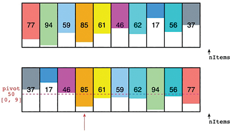
FIGURE 7-6 Partitioning a 10-element array in the AdvancedSorting Visualization tool
The animation starts with a couple of index pointers at the two ends of the range. These indices are moved toward the center, searching for array items that are not in partition order—that is, with a value below the pivot to the left and a value above the pivot to the right. When it finds such a pair, it swaps them. When the two indices eventually meet, the process is done.
In Figure 7-6, items 77 and 37 at the ends were swapped first because they are both on the wrong side of the pivot. Then the lo index advanced to item 94 and the hi index moved left, skipping 56 because it’s above the pivot, and stopped at 17. Items 94 and 17 swap positions, leaving 56 in its original location. The indices move one closer to the middle and continue looking for a pair of items in the wrong partitions. The lo index stops at item 59, and the hi index stops at 46. This pair is swapped and the hunt resumes.
The 59-46 pair turns out to be the last needed to partition them all. Now the first three items of the array are all below the pivot (50), and the last seven items are above it. The tool draws an arrow pointing to item 85 (index 3) to show where the higher partition begins.
It’s not easy to see where the partition will land when you look at the initial array. It depends, of course, on what pivot was chosen and only becomes obvious by going through the swap process. For example, if 90 were the pivot, only item 94 would need to be in the high partition, and the process would be done after 37 and 94 were swapped. Indeed, if you happened to choose certain pivot values, there might not be any items that need to be swapped at all. Even when that happens, however, you still need to find the lowest index of the higher partition. That is an output of this process.
If the pivot were some extreme value, like –10 or 212, then the entire array would be in the same partition. If it were too low, then the result index would be at 0; if it were too high, it would end up at nItems. Let’s look at how to choose the pivot value because it drastically affects the outcome.
After being partitioned, the data is by no means sorted; it has simply been divided into two groups. It’s more sorted, however, than it was before. You can use that improvement to completely sort it with different partitionings, in a manner similar to the way Shellsort used h-sorting. Try running a couple more partitionings using different pivots in the AdvancedSorting Visualization tool. Eventually, the entire array will be sorted. When the data is sorted, partitioning can still be run, but it doesn’t swap any items (except under some rare circumstances we discuss shortly).
Notice that partitioning is not stable. That is, each group is not in the same order it was originally. In fact, partitioning tends to reverse the order of some of the data with equal valued keys in each group. Try inserting some items with duplicate keys into the array and shuffling their positions. Can you find a pivot value that changes their ordering after a partitioning?
The General Partitioning Algorithm
How is the partitioning process carried out? We discuss it in general because it’s useful outside of quicksort. The example shown in the AdvancedSorting Visualization tool is just one kind. The example, however, helps illustrate some important characteristics.
First, note that the partitioning was done within an array by rearranging the items. This means you don’t need to allocate memory for another copy of all the data, which is very useful for large collections.
There must be some test that can be carried out on an item that determines the partition to which it belongs. In the general case, it could be any test such as whether the item’s name contains the letter e. For sorting, you use a pivot value and put everything with a key value less than the pivot in one partition and everything else in the other partition. The pivot doesn’t have to be numeric; it could be any value as long as two values can be compared to see if one is less than the other. The general case of using a partition test function that returns 0 for one partition and 1 for the other is sometimes useful.
As with the insertion sort, which became O(N) when applied to an array that’s already sorted, it’s advantageous to design the algorithm to be fast if the array is already partitioned. For that, we can have a pointer into the array where all the cells to the left are known to be in the lower partition. It would start at index 0 to indicate that none are initially known to be in that partition. Similarly, we set up a second pointer where all the cells to the right are in the higher partition. We initialize it to the last element of the array because none are known to be in that partition either. The idea is to shrink the range between the left and right pointers while moving items into their proper partition.
The core of the algorithm is as follows:
 Increment the left pointer until either we find a cell belonging to the upper partition, or it meets the right index.
- Decrement the right pointer until either we find a cell belonging to the lower partition, or it meets the left index.
- If the left index is at or above the right, the array is already partitioned, so we can return the left index as the end of the lower partition.
- Otherwise, swap items at the left and right indices and partition the range between left and right.
As discussed in Chapter 6, this algorithm can be set up as a recursive algorithm that works on smaller and smaller subranges of the array. Listing 7-2 shows the implementation as a recursive method of the Array class. Like the other sorting algorithms that work on records, you can use a key function to extract the key from the items in the array and partition based on that value’s relationship to the pivot value. Unlike some other algorithms, it allows items whose key exactly matches the pivot to be in either partition. We explain the advantages of that choice after the listing.
LISTING 7-2 The Recursive Partitioning Method of the Quicksort.py Module

def identity(x): return x            # Identity function
import SortArray

class Array(SortArray.Array):        # Base new Array class on SortArray

   def partition_rec(                # Recursively partition array moving
         self,                       # items whose keys are below or equal
         pivot,                      # a pivot value to the left/low side
         lo=0,                       # the rest to the right/high side
         hi=None,                    # within the [lo, hi] range (inclusive)
         key=identity):              # Use key function to extract keys
      if hi is None:                 # Default hi value is last index
         hi = len(self) - 1          # Everything above hi is in upper part
      while (lo <= hi and            # Increment lo until it goes past hi
             key(self.get(lo)) < pivot): # or we find a key that's not
         lo += 1                     # in the lower partition
      while (lo < hi and             # Decrement hi until it matches lo
             pivot < key(self.get(hi))): # or we find the pivot or
         hi -= 1                     # a key not in the upper partition
      if lo >= hi:                   # If lo is at or above hi, then the
         return lo                   # lower partition ends at lo
      self.swap(lo, hi)              # Otherwise, swap the items at lo & hi
      return self.partition_rec(     # and recursively partition remaining
         pivot, lo + 1, hi - 1, key) # items in the array
The partition_rec() method starts by filling in the default value for hi, the index into the array that’s just before the upper partition. At the start, that’s the last index into the array. The lower index, lo, starts at 0, indicating that no cells of the array have been found to have keys below the pivot. The cells between lo and hi need to be partitioned and form the range to be shrunk.
The first while loop implements the first step of the core algorithm. It increments lo until either lo > hi or the cell at lo has a key that is greater than or equal to the pivot, which means it belongs in the upper partition. The second while loop implements the second step of decrementing hi until it either goes past lo or the cell at hi has a key indicating it should be in the lower partition.
Note that the comparisons are slightly different in the two while loops. The first loop must use lo <= hi rather than lo < hi to ensure that the value at lo is checked against the pivot, and lo is incremented if there is only one cell in the range, that is, lo == hi. It’s important to increment lo to point past hi if the entire array belongs in the lower partition. Using lo < hi in the first loop condition would mean the loop body is not entered, and lo could end up pointing to a cell with a key below the pivot. The second loop, however, uses lo < hi in its loop condition because when lo == hi, you know that the cell at that index must belong in the upper partition.
After lo and hi have been moved to narrow the range of unchecked cells, the if statement checks whether the range is one or fewer cells in length. If so, there’s nothing to swap, and it can return lo as the index that is just above the lower partition. This is the base case for this recursive algorithm. If the range is bigger than one, then the values at lo and hi are swapped (using the swap() method defined in the SortArray class of Chapter 3). The recursive call partitions the range between the two swapped values.
Converting the recursive version of the partitioning algorithm to a loop version is easier than the general case. The reasons that it’s simpler are
- The program doesn’t do anything with the returned value of the recursive call other than return it to its caller, and
- The values of the parameters—
pivot,lo, andhi—don’t need to be saved and restored between calls.
With these two conditions, you don’t need a stack of problem descriptions; you only need to update the lo and hi variables as the range of cells to check is reduced. Listing 7-3 shows the loop version of the method, partition().
LISTING 7-3 The Loop-Based Partitioning Method of the Quicksort.py Module
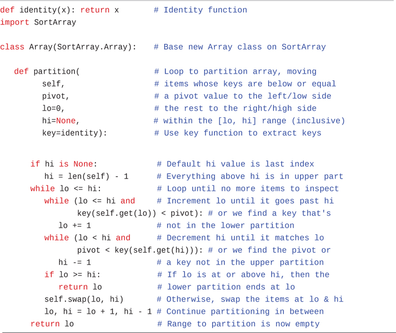
def identity(x): return x        # Identity function
import SortArray

class Array(SortArray.Array):    # Base new Array class on SortArray

   def partition(                # Loop to partition array, moving
         self,                   # items whose keys are below or equal
         pivot,                  # a pivot value to the left/low side
         lo=0,                   # the rest to the right/high side
         hi=None,                # within the [lo, hi] range (inclusive)
         key=identity):          # Use key function to extract keys
      if hi is None:             # Default hi value is last index
         hi = len(self) - 1      # Everything above hi is in upper part
      while lo <= hi:            # Loop until no more items to inspect
         while (lo <= hi and     # Increment lo until it goes past hi
                key(self.get(lo)) < pivot): # or we find a key that's
            lo += 1              # not in the lower partition
         while (lo < hi and      # Decrement hi until it matches lo
                pivot < key(self.get(hi))): # or we find the pivot or
            hi -= 1              # a key not in the upper partition
         if lo >= hi:            # If lo is at or above hi, then the
            return lo            # lower partition ends at lo
         self.swap(lo, hi)       # Otherwise, swap the items at lo & hi
         lo, hi = lo + 1, hi - 1 # Continue partitioning in between
      return lo                  # Range to partition is now empty
In the loop-based method, the lo and hi parameters become local variables that are initialized at the beginning. Instead of recursive calls, a new outer while loop is added that iterates until the [lo, hi] range becomes empty. Inside that loop, the logic is nearly identical to the recursive version. The lo and hi indices move up and down like before. The next three lines of code—checking on the size of the remaining range, returning lo if the range is too small, and swapping the values at lo and hi—are identical to the recursive version. The difference comes at the end where lo and hi are updated (the way they would have been changed in the recursive call), and there is a return lo statement if the outer loop completes with an empty range.
Testing the partitioning method on a 10-element array with two different pivots shows:

Initialized array contains [77, 94, 59, 85, 61, 46, 62, 17, 56, 37]
Partitioning an array of size 10 around 61 returns 5
                                                V
Partitioned array contains [37, 56, 59, 17, 46, 61, 62, 85, 94, 77]

Initialized array contains [37, 56, 59, 17, 46, 61, 62, 85, 94, 77]
Partitioning an array of size 10 around 46 returns 2
                                    V
Partitioned array contains [37, 17, 59, 56, 46, 61, 62, 85, 94, 77]
The V in the output is pointing to the index of the first cell in the upper partition, that is, the index returned by the partition() method. You can see that the partitions are successful: the numbers to the left of the returned index are all smaller than the pivot values of 61 and 46, respectively. Note that the sizes of the partitions depend on the choice of pivot. Only those array cells that had to be swapped were affected, for example, only the values of 17 and 56 in the second example that pivoted around 46. The first partition had already swapped 77 and 37, 94 and 56, 85 and 17, and 61 and 46.
Equal Keys
Somewhat surprisingly, it doesn’t matter if items whose key matches the pivot go in the lower or higher partition. The pivot value is the dividing line between the two partitions. Items that have a key equal to the pivot could be considered to belong to either one.
In the partition() method in Listing 7-3, both loops that increment the lo and decrement the hi indices stop when they find an item with the pivot as its key (in addition to finding an item belonging in the opposite partition). If the indices differ after going through both loops, then the items they index are swapped. If both items have a key equal to the pivot, there is no need to swap them. So, shouldn’t the algorithm skip the swap if it finds equal keys? The answer is not so straightforward.
To add such a test would put another comparison in the loop that would be run once for every iteration of the outer loop. It would save the expense of a swap, but only if the data has keys of equal value, and both are equal to the pivot. That’s not likely to happen, in general. Furthermore, it would save significant time only if the cost of swapping two items in the array were much more than comparing the keys.
There’s another, more subtle reason to swap the items even when one or both has a key equal to the pivot. If the algorithm always puts items whose keys match the pivot in one partition, say the higher one, then it can decrement the hi index past those items as it looks for items to swap. Doing so moves the eventual partition index to the lowest possible value and minimizes swaps. As discussed later in the section on quicksort, it’s good for the partition indices to end up in the middle of the array and very bad for them to end up at the ends. The idea is somewhat similar to binary search: dividing the range in half is most efficient because it limits the maximum size of the remaining ranges to search.
Efficiency of the Partition Algorithm
The partition algorithm runs in O(N) time. It’s easy to see why this is so when running the Partition operation in the Visualization tool: the two pointers start at opposite ends of the array and move toward each other, stopping and swapping as they go. When they meet, the partition is complete. Each cell of the array is visited at most one time, either by the lo or the hi pointer. If there were twice as many items to partition, the pointers would move at the same rate, but they would have twice as many items to compare and swap, so the process would take twice as long. Thus, the running time is proportional to N.
More specifically, partitioning an N-cell array makes exactly N comparisons between keys and the pivot value. You can see that by looking at the code where the key() function is called and its value compared with the pivot. There’s one test with the item at the lo pointer and one with the hi pointer. Because lo and hi are checked prior to those comparisons, you know that either lo < hi or that the comparison with the pivot and the key at hi doesn’t happen. The lo and hi values range over all N cells.
The lo and hi pointers are compared with each other N + 2 times because that comparison must succeed for each of the pivot comparisons to happen, and they must each fail when they find either a pair to swap or find each other. The number of comparisons is independent of how the data is arranged (except for the uncertainty between one or two extra comparisons at the end of the process).
The number of swaps, however, does depend on how the input data is arranged. If it’s inversely ordered, and the pivot value divides the items in half, then every pair of values must be swapped, which is N/2 swaps.
For random data, there are fewer than N/2 swaps in a partition, even if the pivot value is such that half the items are shorter and half are taller. The reason is that some items are already in the right place (short bars on the left, tall bars on the right in the visualization). If the pivot value is higher (or lower) than most of the items, there will be even fewer swaps because only those few items that are higher (or lower) than the pivot will need to be swapped. On average, for random data with random pivots, about half the maximum number of swaps take place.
Although there are fewer swaps than comparisons, they are both proportional to N. Thus, the whole partitioning process runs in O(N) time.
Quicksort
Quicksort is a popular sorting algorithm, and for good reason: in the majority of situations, it’s the fastest, operating in O(N×log N) time, and only needs O(log N) extra memory. C. A. R. (Tony) Hoare discovered quicksort in 1962.
To understand quicksort, you should be familiar with the partitioning algorithm described in the preceding section. Basically, the quicksort algorithm operates by partitioning an array into two subarrays and then calling itself recursively to quicksort each of these subarrays. There are some embellishments, however, to be made to this basic scheme. They have to do with the selection of the pivot and the sorting of small partitions. We examine these refinements after we look at a simple version of the main algorithm.
It’s difficult to understand what quicksort is doing before you understand how it does it, so we reverse our usual presentation and show the Python code for quicksort before presenting the visualization tool.
The Basic Quicksort Algorithm
The code for a basic recursive quicksort method is fairly simple. Listing 7-4 shows a sketch of the algorithm.
LISTING 7-4 A Sketch of the Quicksort Algorithm in Python

   def quicksort_sketch(        # Sort items in an array between lo
         self, lo=0, hi=None,   # and hi indices using Hoare's
         key=identity):         # quicksort algorithm on the keys
      if hi is None:            # Fill in hi value if not specified
         hi = len(self) - 1
      if lo >= hi:              # If range has 1 or fewer cells,
         return                 # then no sorting is needed

      pivot = self.choosePivot(lo, hi) # Choose a pivot

      hipart = self.partition(  # Partition array around the key
         key(pivot),            # of the item at the pivot index and
         lo, hi, key)           # record where high part starts

      self.quicksort_sketch(lo, hipart - 1, key) # Sort lower part
      self.quicksort_sketch(hipart, hi, key) # Sort higher part
As you can see, there are five basic steps:
Check the base case and return if the [sub]array is small enough.
Choose a pivot.
Partition the subarray into lower and higher parts around the pivot.
Make a recursive call to sort the lower part.
Make another recursive call to sort the higher part.
The first lines should look familiar from other recursive routines. Like the partition_rec() method in Listing 7-2, the lo and hi indices are the leftmost and rightmost cells of the array to be sorted. If not provided by the caller, they are set to be the first and last cells of the full array. Testing for the base case involves seeing whether there are two or more cells to be sorted. If there are one or zero, then no sorting is needed, and the method returns immediately.
The sketch shows a call to choosePivot() to select a pivot item in the subarray. We return to that choice in a moment, but for now, assume that it randomly chooses one of the items between the lo and hi cells. After the partition, all the items in the left subarray, below hipart, are smaller than or equal to all those on the right. If you then sort the left subarray and the right subarray, the entire array will be sorted. How do you sort these subarrays? By calling this very method recursively.
When quicksort_sketch() is called on something other than the base case, the algorithm chooses a pivot value and calls the partition() method, described in the preceding section, to partition it. This method returns the index number of the first cell in the higher partition. That index gets stored in the hipart variable and is used to determine the subarrays to be recursively sorted. The situation is shown in Figure 7-7 with a “randomly” chosen pivot of 38.
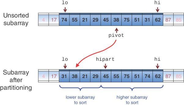
FIGURE 7-7 Partitioning in one call to quicksort_sketch()
Note that the pivot doesn’t necessarily end up being moved to the beginning or end of its partition. Nor does it always stay where it started. After the subarray is partitioned, quicksort_sketch() calls itself recursively, once for the lower part of its array, from lo to hipart - 1, and once for the higher part, from hipart to hi. These calls move the pivot item (and all other items) into their sorted positions.
Choosing a Pivot Value
What pivot value should the quicksort algorithm use? Here are some relevant ideas:
- The pivot value should be the key value of an actual data item; this item is also called the pivot. At a minimum, avoiding an extreme value outside the range of keys prevents making empty partitions, but it also allows for some other optimizations.
- You can pick a data item to be the pivot somewhat arbitrarily. For simplicity, you could always pick the item on the right end of the subarray being partitioned.
- After the partition, if the pivot is inserted at the boundary between the lower and upper subarrays, it will be in its final sorted position.
This last point may sound unlikely, but remember that, because the pivot’s key value is used to partition the array, following the call to partition() the lower subarray holds items with keys equal to or smaller than the pivot, and the right subarray holds items with keys equal to or larger. If the pivot could somehow be placed between these two subarrays, it would be in the correct place—that is, in its final sorted position. Figure 7-8 shows how this looks with the pivot example value of 38.
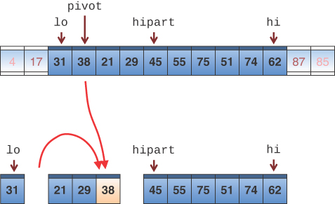
FIGURE 7-8 Moving the pivot between the subarrays
This figure is somewhat fanciful because you can’t actually slice up the array as shown, at least not without copying a lot of cells. So how do you move the pivot to its proper place?
You could shift all the items in the left subarray to the left one cell to make room for the pivot. This approach is inefficient, however, and unnecessary. You can select the pivot to be any item from the array. If you select the rightmost one and partition everything to the left of it, then you can simply swap the pivot with the item indexed by hipart—the leftmost of the higher part as shown in Figure 7-9. In fact, doing so brings the array one step closer to being fully sorted. This swap places the pivot in its proper position between the left and right groups. The 75 is switched to where the pivot was, and because it remains in the right (higher) group, the partitioning is undisturbed. Note that in choosing the rightmost cell of the subarray—the one at the hi index—it must be excluded from the range that the partition() method reorganizes because it shouldn’t be swapped for any other item.

FIGURE 7-9 Swapping the pivot from the right
Similarly, the pivot could be chosen as the leftmost cell and then swapped into position just to the left of hipart. In either case, the swap might not be needed if the partitioning left no cells in the higher or lower partition, respectively. Because the pivot can be placed in either partition, these methods can be used to guarantee that there will be at least one cell in the higher or lower partition, respectively.
Swapping the pivot with the value at the start of the higher partition ensures the pivot ends up in its final resting place. All subsequent activity will take place on one side of it or on the other, but the pivot itself won’t be moved again. In fact, you can exclude it from the subrange in the recursive call to sort the higher range—for example:
      self.quicksort_sketch(lo, hipart - 1, key) # Sort lower part
      self.quicksort_sketch(hipart + 1, hi, key) # Sort higher part
By removing that one cell from subsequent processing, the algorithm guarantees that the subranges are always diminishing. To see that, think about the range for hipart. It could have any value from lo to hi (but not hi + 1 because you chose the pivot to be equal to the key at hi). At those extreme values, one of the recursive subranges will be empty while the other will have one fewer cell than the original lo to hi range—either [lo, hi – 1] or [lo + 1, hi].
We can make an optimization to the partitioning algorithm by taking advantage of the constraint that there will always be at least one item that belongs in the high partition. That constraint means the test for the end of the first loop—the one that advances lo to find a higher partition item—can be simplified. It no longer needs to check that lo <= hi because the second part of the test checking the key at lo versus the pivot must fail when lo == hi. Although this comparison test might seem trivial, it occurs in the innermost loop of what could be a very long calculation, so saving a few operations here can have a large impact. There are a few more improvements in the full implementation in the following sections.
A First Quicksort Implementation
To flesh out the embellishments to the sketch shown earlier, we provide a working version, called the qsort() method, in Listing 7-5. This method captures the algorithm just described, along with its revised partitioning method.
LISTING 7-5 The qsort() Method with Improved Partitioning
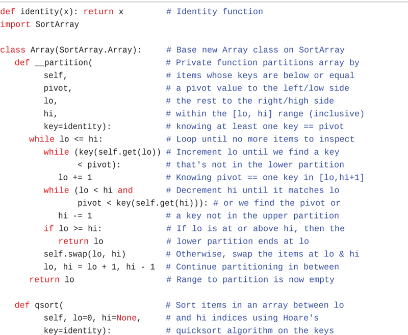
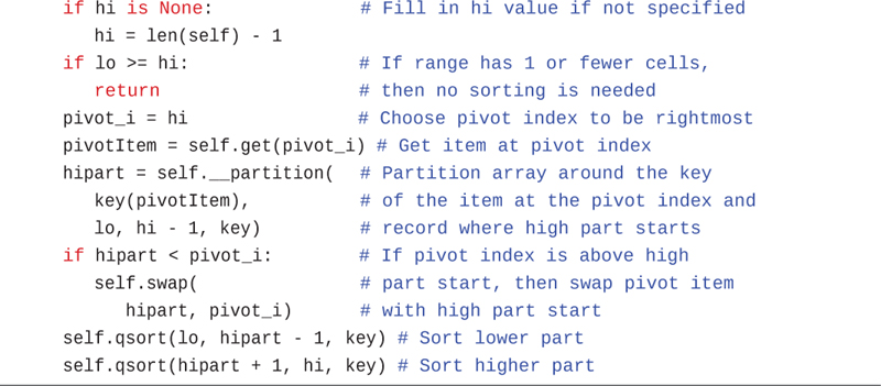
def identity(x): return x         # Identity function
import SortArray

class Array(SortArray.Array):     # Base new Array class on SortArray
   def __partition(               # Private function partitions array by
         self,                    # items whose keys are below or equal
         pivot,                   # a pivot value to the left/low side
         lo,                      # the rest to the right/high side
         hi,                      # within the [lo, hi] range (inclusive)
         key=identity):           # knowing at least one key == pivot
      while lo <= hi:             # Loop until no more items to inspect
         while (key(self.get(lo)) # Increment lo until we find a key
                < pivot):         # that's not in the lower partition
            lo += 1               # Knowing pivot == one key in [lo,hi+1]
         while (lo < hi and       # Decrement hi until it matches lo
                pivot < key(self.get(hi))): # or we find the pivot or
            hi -= 1               # a key not in the upper partition
         if lo >= hi:             # If lo is at or above hi, then the
            return lo             # lower partition ends at lo
         self.swap(lo, hi)        # Otherwise, swap the items at lo & hi
         lo, hi = lo + 1, hi - 1  # Continue partitioning in between
      return lo                   # Range to partition is now empty

   def qsort(                     # Sort items in an array between lo
         self, lo=0, hi=None,     # and hi indices using Hoare's
         key=identity):           # quicksort algorithm on the keys
      if hi is None:              # Fill in hi value if not specified
         hi = len(self) - 1
      if lo >= hi:                # If range has 1 or fewer cells,
         return                   # then no sorting is needed
      pivot_i = hi                # Choose pivot index to be rightmost
      pivotItem = self.get(pivot_i) # Get item at pivot index
      hipart = self.__partition(  # Partition array around the key
         key(pivotItem),          # of the item at the pivot index and
         lo, hi - 1, key)         # record where high part starts
      if hipart < pivot_i:        # If pivot index is above high
         self.swap(               # part start, then swap pivot item
            hipart, pivot_i)      # with high part start
      self.qsort(lo, hipart - 1, key) # Sort lower part
      self.qsort(hipart + 1, hi, key) # Sort higher part
Because the partitioning method now relies on the pivot value always being a key of one of the cells between lo and hi, we have made it a private method, __partition(), so that it cannot be called by the users of this Array class using some other pivot value. The enhancement comes in the second while loop of __partition(), by getting rid of the test for lo <= hi. It still needs the test for lo < hi in the third while loop because there is no guarantee that it will find an item in the lower partition before running in to lo. If the pivot value was the lowest key in the whole array and distinct, all the items would satisfy the pivot < key(self.get(hi)) test. Because this is a private method that is only called by qsort(), we can also remove the default values for the lo and hi parameters since the qsort() method always provides them.
The qsort() method remains recursive (although it could be converted to a loop-based algorithm as you’ve seen). It tracks both the index to the pivot item and the item itself in different variables, pivot_i and pivotItem. It replaces the call to choosePivot() with a simple assignment to improve efficiency slightly. Because the pivot is the rightmost item, it calls the private __partition() method with the range [lo, hi – 1] to prevent the pivot from being swapped. After partitioning, it swaps the pivot item and the item at the start of the higher partition. That swap needs to be done only if the pivot index is higher than the first index of that part, hipart. The method ends with the recursive calls on the lower and higher parts, excluding the pivot item that was moved to the cell at hipart.
You can add a print statement to the qsort() method right after the partitioning to see what’s happening. By adding the line
print('Partitioning', lo, 'to', hi, 'leaves', self)
you can see the ranges being partitioned and the changes in the values of the array. Placing this print statement after the partitioning and swapping of the pivot are done (just before the recursive calls to sort the lower and higher parts), along with an initial printing of the array contents, produces the output in Listing 7-6.
LISTING 7-6 Output of qsort() with a print Statement
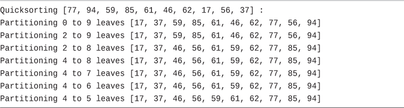
Quicksorting [77, 94, 59, 85, 61, 46, 62, 17, 56, 37] :
Partitioning 0 to 9 leaves [17, 37, 59, 85, 61, 46, 62, 77, 56, 94]
Partitioning 2 to 9 leaves [17, 37, 59, 85, 61, 46, 62, 77, 56, 94]
Partitioning 2 to 8 leaves [17, 37, 46, 56, 61, 59, 62, 77, 85, 94]
Partitioning 4 to 8 leaves [17, 37, 46, 56, 61, 59, 62, 77, 85, 94]
Partitioning 4 to 7 leaves [17, 37, 46, 56, 61, 59, 62, 77, 85, 94]
Partitioning 4 to 6 leaves [17, 37, 46, 56, 61, 59, 62, 77, 85, 94]
Partitioning 4 to 5 leaves [17, 37, 46, 56, 59, 61, 62, 77, 85, 94]
The first call to the qsort() method operates on the full array, the range [0, 9]. The pivot is the rightmost item, whose value is 37. The only item lower than that is item 17 at index 7. The partitioning swaps the 77 from the leftmost cell with the 17 and then swaps the pivot value 37 with the item at index 1 (the value of hipart after partitioning), which is item 94. Now the array has items equal to and below 37 in the range [0, 0] and the items equal to and higher in the range [1, 9] (the hipart starts at index 1 and includes the pivot).
The recursive call to sort the lower range ends up being a base case requiring no action. The call to sort the higher range [2, 9] is the next output line. Note that the pivot from the first call, 37, has been removed from the range because it’s known to be in the correct position, index 1. In the range [2, 9], the pivot is 94. Because that is the maximum value of the range, the partitioning makes no changes. The pivot remains at the right end, and the lower partition is sorted next.
The third Partitioning output line shows sorting the range below the pivot, 94, which spans [2, 8]. This time the pivot is 56. There is one item less than the pivot, and that is 46 at index 5. That value gets swapped with the leftmost value, 59, at index 2. Then the pivot is swapped with the leftmost item of the higher partition, 85. That leaves the lower partition as [2, 2] and the higher partition as [3, 8].
The fourth Partitioning output line in Listing 7-6 shows sorting the higher range [4, 8], ignoring the pivot of the previous call. The pivot at index 8 is 85; the value that was swapped with the pivot of the previous call. Because 85 is the maximum value of that range, no swaps are made, and only the lower partition is a non-base case.
The fifth Partitioning output line sorts the lower partition range, [4, 7]. The pivot is 77 for that range, which again is a maximum, so no swaps are made. The sixth output line sorts the next lower partition range [4, 6]. Here the pivot is 62, and again it’s the maximum of that range, so it’s on to sort the lower partition.
The seventh call works on the lower partition of the sixth call, the range [4, 5]. The pivot for that range is 59, which is less than the only other item, 61. That pivot gets swapped with the 61 because that is where hipart starts. Because the range has only two cells, the recursive calls are base cases that make no more changes.
Was that approach efficient? The particular array processed in Listing 7-6 generated seven calls to the __partition() method. That’s quite a few when compared to the 10 elements in the array. This is close to the worst-case behavior, which we analyze a little later. In general, however, the pivots are likely to split long ranges in approximately equal subranges, making the algorithm very fast.
Running Quicksort in the AdvancedSorting Visualization Tool
At this point you know enough about the quicksort algorithm to run some examples in the Visualization tool. The code in the Visualization tool runs a version of the algorithm with some optimizations that we haven’t discussed yet. The first thing to do is to ensure the check box labeled “Use median of 3” below the Quicksort button is unchecked. We get to that optimization a little later, along with some others.
With the Median of 3 option turned off, run the quicksort on an array. Figure 7-10 shows the final result after the quicksort finishes. As the quicksort process runs, you see the partition lines appear as it processes the subarrays. The first call to quicksort runs on the full range of the array, cells 0 through 9 in the 10-element array of Figure 7-10. If you look carefully, you can see that it chooses the rightmost item in each subarray as the pivot. The pivot line for each partition shows during the partitioning but then disappears.
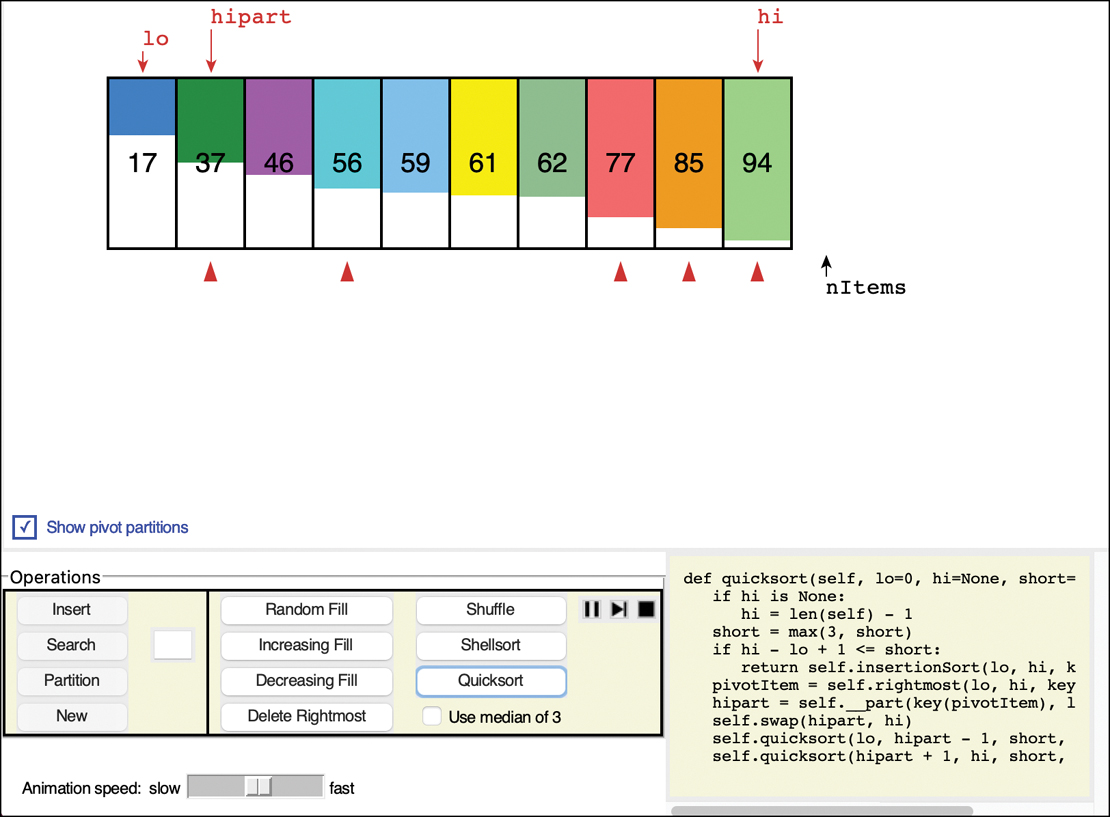
FIGURE 7-10 The result of quicksort in the AdvancedSorting Visualization tool
At the end of each partitioning, a triangle is placed below the first cell of the higher partition, similar to the arrow that the Partition button left. These triangles remain after the sort is complete to show where each partition landed.
In Figure 7-10, the last item of the initial array, 37, was the first pivot value, and led to placing the triangle below cell 1. Only item 17 is lower, and the other nine items were placed in the higher partition. The quicksort runs the partitioning four more times, placing the other triangles to show where it split the subarrays. You can hide or show the triangles by selecting the check box labeled “Show pivot partitions.”
As you watch the animation of the quicksort process, you can easily see how the ranges are split at the hipart index, followed by processing of the left and right partitions. When the size of partitions grows small, it does some special processing that we describe a little later.
One of the key things to watch is how many partitions are made. The number of triangles showing at the end provides the count. You want to make as few partitions as possible to make the sorting process efficient. Try making a larger array, filled with random values, and quicksorting it (with the Median of 3 option still turned off). Figure 7-11 shows an example with a 77-element array that led to 29 partitions.
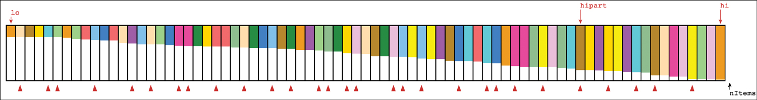
FIGURE 7-11 Running quicksort on a 77-element array choosing the rightmost as pivot
While you watch the sorting animation, compare it to what you saw with the Shellsort. Does it appear to be generally “more sorted” with each partitioning?
The Details
Figure 7-12 shows all the steps involved in sorting a 12-element array using qsort(). The horizontal brackets under the arrays show which subarray is being partitioned at each recursive call, along with a call number. Some calls are on single element or empty ranges; these are the base cases that return immediately and have no arrow indicating a pivot was chosen. The pivots are highlighted as they are placed in their final positions.

FIGURE 7-12 The qsort process
Sometimes, as in calls 6, 9, and 12, the pivot ends up in its original position on the right side of the subarray being sorted. In this situation, after sorting the subarray to the left of the pivot, the subarray to the right doesn’t need to be sorted because it is empty. There still is a call to the qsort() method, as indicated by the call numbers in the figure that have no bracketed range—calls 8, 14, and 15.
The different calls in Figure 7-12 occur at different levels (or depths) of recursion, as shown in the table on the right. The first call to qsort() is at the first level. It makes two recursive calls to sort the subarrays to the left and the right of its pivot, 56. Those calls are at level 2, and they make calls for the lower and higher partitions that they create. The level 1 call to sort its lower partition is call 2 and covers indices 0 through 5. The call to sort its higher partition ends up being call 9 on indices 7 through 11. The intervening calls are all the deeper recursive calls to finish sorting the lower partition.
The order in which the partitions are created, corresponding to the call numbers, does not correspond with depth. It’s not the case that all the first-level partitions are done first, then all the second-level ones, and so on. Instead, the left group at every level is handled before any of the right groups.
The number of levels in the table shows that with 12 data items, the machine stack needs enough space for five sets of arguments and return values—one for each recursion level. This is, as you see later, somewhat greater than the logarithm to the base 2 of the number of items: log2N. The size limit of the machine stack varies between systems. Sorting very large numbers of data items using recursive procedures may cause this stack to overflow.
Degenerates to O(N2) Performance
Try the following example using the AdvancedSorting Visualization tool. Make an empty array of 10 to 20 cells and use the Increasing Fill button to fill them with a sequence of increasing keys. Then run the quicksort with the Median of 3 option turned off. You’ll see that it seems to create more triangles for the partitions. A 10-item array creates 7 triangles, and a 20-item array creates 17. What’s happening here?
The problem is in the selection of the pivot. Ideally, the pivot should be the median of the items being sorted. That is, half the items should be larger than the pivot, and half smaller. That choice would result in the array being partitioned into two subarrays of equal size. Having two equal subarrays is the optimum situation for the quicksort algorithm. If it sorts one large and one small array, the quicksort is less efficient because the larger subarray must be subdivided more times. That also requires more recursive levels.
The worst situation results when a subarray with N cells is divided into one subarray with 1 cell and the other with N–1 cells. This division into 1 cell and N–1 cells can be seen in calls 6, 9, and 12 of Figure 7-12. In the visualization tool, it happens in every partition (except that three cells don’t get partitioned, which we explain in a moment).
If this 1 and N–1 division happens with every partition, then every cell requires a separate partition step. This is, in fact, what takes place when the input data is already sorted (or inversely sorted). In all the subarrays, the pivot is the largest (or smallest) item. If it’s the largest item, the partitions are of size N–1 and 1, the pivot (assuming no duplicate keys). If the pivot is the smallest item, all the cells go in the larger partition, and the recursive calls are made on an empty subarray and one of size N–1, and the pivot must be swapped into final position (leading to the largest remaining item being the pivot on the next call).
As you can see in the Visualization tool, the triangles for the pivot points are next to one another, which means one partition ended up being a single cell. In this situation, the advantage gained by the partitioning process is lost, and the performance of the algorithm degenerates to O(N2).
Besides being slow, there’s another potential problem when quicksort operates in O(N2) time. When the number of partitions increases, the number of recursive method calls also increases. In the ideal case, the number of method calls is O(log2 N), but in this worst situation, it becomes O(N). Every function or method call takes up room on the machine stack. If there are too many calls, the machine stack may overflow and paralyze the system. Even if you convert the recursive procedure to an explicit stack approach, O(N) memory will be consumed to hold the information needed to correctly process the subranges.
To summarize: the qsort() method chooses the rightmost item’s key as the pivot. If the data is truly random, this choice isn’t too bad because usually the pivot isn’t too close to either extreme value of the keys. When the input data is (inversely) sorted, however, choosing the pivot from one end or the other is a bad idea. How can we improve on this approach to selecting the pivot?
Median-of-Three Partitioning
Many schemes have been devised for picking a better pivot. The method of choosing an item at random is simple, but—as you’ve seen—doesn’t always result in a good selection. Choosing items with keys at or near the extreme ends of the range of keys leads to unbalanced partitions. Alternatively, you could examine all the items and actually calculate which of their keys was the median. This pivot choice would be ideal, but doing so isn’t practical because it could take more time than the sort itself.
A compromise solution is to examine the first, last, and middle items of the subarray, and use the median of their keys for the pivot. Picking the median of the first, last, and middle elements is called the median-of-three approach and is shown in Figure 7-13.
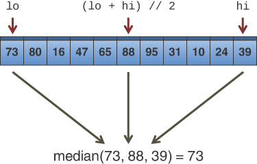
FIGURE 7-13 The median of three
Finding the median of three items is obviously much faster than finding the median of all the items, and yet it successfully avoids picking the largest or smallest item in cases where the input data is already sorted or inversely sorted. There are probably some pathological arrangements of data where the median-of-three scheme works poorly, but normally it’s a fast and effective technique for finding the pivot.
Besides picking the pivot more effectively, the median-of-three approach has an additional benefit: you can dispense with the lo < hi test in the second inner while loop, leading to a small increase in the algorithm’s speed. How is this possible?
You can eliminate this test because you can use the median-of-three approach to not only select the pivot but also to sort the three elements used in the selection process. Figure 7-14 shows this operation.
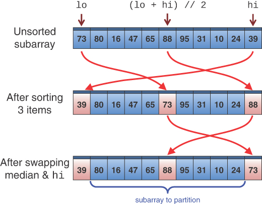
FIGURE 7-14 Sorting the left, center, and right elements
When these three elements are sorted, and the median item is selected as the pivot, you are guaranteed that the element at the left end of the subarray is less than (or equal to) the pivot, and the element at the right end is greater than (or equal to) the pivot. This means that the lo and hi indices can’t step beyond the right or left ends of the array, respectively, even if you remove the lo < hi test (and the lo <= hi test that was previously removed from the first inner loop).
Removing that test may not seem like a wise idea, especially with the swaps that happen during the partitioning algorithm. On closer inspection, however, those swaps only move lower items to the left and higher items to the right, so there will always be a key that causes the two loops to stop. These items are called sentinels because they guard against going out of bounds. The hi index will stop decrementing, thinking it needs to swap the item, only to find that it may have already crossed the lo index and the partition is complete.
Another small benefit to median-of-three partitioning is that after the left, middle, and right elements are sorted, and the median is swapped with the rightmost item, the partition process doesn’t need to examine the lowest and median elements again. The partition can begin at lo+1 and hi-1 as shown in the last row of Figure 7-14 because lo and hi have, in effect, already been partitioned. You know that lo is in the correct partition because it’s on the left and it’s less than or equal to the pivot, and hi is in the correct place because it’s on the right and it is the pivot. Neither one may be in its final, sorted position, but all that matters is that they are partitioned correctly at this point.
Thus, median-of-three partitioning not only avoids O(N2) performance for already-sorted data but also allows you to speed up the inner loops of the partitioning algorithm and slightly reduces the number of items that must be partitioned.
Handling Small Partitions
Using the median-of-three pivot selection method, it follows that the quicksort algorithm won’t work for partitions with fewer than three items. With exactly three items, the median-of-three would fully sort the items and then perform two unnecessary swaps of the median and high items. Performing these extra swaps seems wasteful, so finding another method for processing three or fewer items seems appropriate. The number 3 in this case is called a cutoff point. What is the best way to process these small subarrays? Would it be wise to apply the nonmedian choice of pivot as we did before in qsort()? Are there other sorting methods that might do better with small subarrays?
Using an Insertion Sort for Small Partitions
One option for dealing with small partitions is to use the insertion sort. That approach works for any size subarray and has the added benefit of being O(N) for already-sorted subarrays. In fact, you aren’t restricted to a cutoff of 3. You could set the cutoff to 10, 20, or any other number 3 or higher, expecting to find some optimum value. It’s interesting to experiment with different values of the cutoff to see where the best performance lies. Knuth (see Appendix B) recommended a cutoff of 9. The optimum number is usually more than 3 and depends on a variety of factors: the kinds of input data distributions that happen frequently, the computer, the operating system, the compiler (or interpreter), and so on.
The Full Quicksort Implementation
Combining all these improvements into the implementation results in the full quicksort() method shown in Listing 7-7. It has its own private partitioning method, __part(), that includes the optimizations in the loop conditions based on the sentinel values from the median-of-three algorithm.
LISTING 7-7 The full quicksort() Method for Sorting Arrays
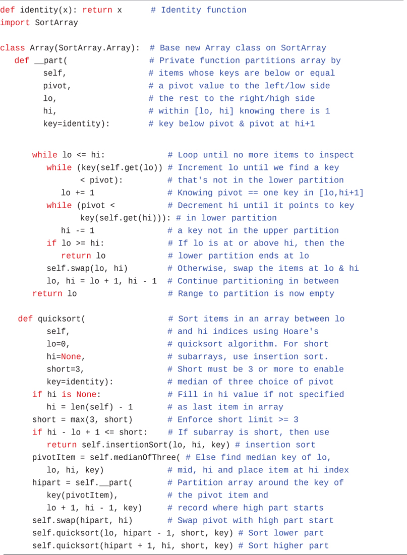
def identity(x): return x      # Identity function
import SortArray

class Array(SortArray.Array):  # Base new Array class on SortArray
   def __part(                 # Private function partitions array by
         self,                 # items whose keys are below or equal
         pivot,                # a pivot value to the left/low side
         lo,                   # the rest to the right/high side
         hi,                   # within [lo, hi] knowing there is 1
         key=identity):        # key below pivot & pivot at hi+1
      while lo <= hi:             # Loop until no more items to inspect
         while (key(self.get(lo)) # Increment lo until we find a key
                < pivot):         # that's not in the lower partition
            lo += 1               # Knowing pivot == one key in [lo,hi+1]
         while (pivot <           # Decrement hi until it points to key
                key(self.get(hi))): # in lower partition
            hi -= 1               # a key not in the upper partition
         if lo >= hi:             # If lo is at or above hi, then the
            return lo             # lower partition ends at lo
         self.swap(lo, hi)        # Otherwise, swap the items at lo & hi
         lo, hi = lo + 1, hi - 1  # Continue partitioning in between
      return lo                   # Range to partition is now empty

   def quicksort(                 # Sort items in an array between lo
         self,                    # and hi indices using Hoare's
         lo=0,                    # quicksort algorithm. For short
         hi=None,                 # subarrays, use insertion sort.
         short=3,                 # Short must be 3 or more to enable
         key=identity):           # median of three choice of pivot
      if hi is None:              # Fill in hi value if not specified
         hi = len(self) - 1       # as last item in array
      short = max(3, short)       # Enforce short limit >= 3
      if hi - lo + 1 <= short:    # If subarray is short, then use
         return self.insertionSort(lo, hi, key) # insertion sort
      pivotItem = self.medianOfThree( # Else find median key of lo,
         lo, hi, key)             # mid, hi and place item at hi index
      hipart = self.__part(       # Partition array around the key of
         key(pivotItem),          # the pivot item and
         lo + 1, hi - 1, key)     # record where high part starts
      self.swap(hipart, hi)       # Swap pivot with high part start
      self.quicksort(lo, hipart - 1, short, key) # Sort lower part
      self.quicksort(hipart + 1, hi, short, key) # Sort higher part
The quicksort() method has a new, optional parameter, short, which determines the cutoff for using insertion sort on short subarrays. It defaults to 3 but can be set higher. (The AdvancedSorting Visualization tool uses the default value of 3.) The base case test is modified to look for subarrays that have short or fewer cells in them. They are processed by the insertionSort() method shown in Listing 7-8.
If you compare these two methods to their counterparts in the earlier implementation shown in Listing 7-5, they are similar. The small changes do not reduce (or significantly increase) the complexity of the program. They do, however, result in a big impact on the performance.
Listing 7-8 shows the helper methods used by quicksort(). The medianOfThree() method performs a three-element sort at the low, middle, and high indices of the subarray. Because the number of items to sort is known and small, it’s better to write a few if statements to swap values than to make a loop-based sorting routine. After computing the index of the middle item, mid, the first two if statements swap items to place the item with the lowest key at the lo position. Normally for a sort, the next step would be to compare the other two items and ensure the item with the highest key is placed at hi. Because this method is preparing the data for partitioning, however, the item with the middle key is placed at hi. It returns that item because it is the median of the three keys.
LISTING 7-8 The Helper Methods for quicksort()
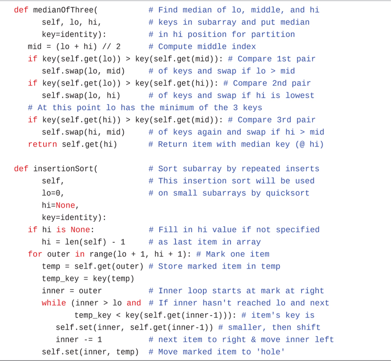
   def medianOfThree(           # Find median of lo, middle, and hi
         self, lo, hi,          # keys in subarray and put median
         key=identity):         # in hi position for partition
      mid = (lo + hi) // 2      # Compute middle index
      if key(self.get(lo)) > key(self.get(mid)): # Compare 1st pair
         self.swap(lo, mid)     # of keys and swap if lo > mid
      if key(self.get(lo)) > key(self.get(hi)): # Compare 2nd pair
         self.swap(lo, hi)      # of keys and swap if hi is lowest
      # At this point lo has the minimum of the 3 keys
      if key(self.get(hi)) > key(self.get(mid)): # Compare 3rd pair
         self.swap(hi, mid)     # of keys again and swap if hi > mid
      return self.get(hi)       # Return item with median key (@ hi)

   def insertionSort(           # Sort subarray by repeated inserts
         self,                  # This insertion sort will be used
         lo=0,                  # on small subarrays by quicksort
         hi=None,
         key=identity):
      if hi is None:            # Fill in hi value if not specified
         hi = len(self) - 1     # as last item in array
      for outer in range(lo + 1, hi + 1): # Mark one item
         temp = self.get(outer) # Store marked item in temp
         temp_key = key(temp)
         inner = outer          # Inner loop starts at mark at right
         while (inner > lo and  # If inner hasn't reached lo and next
                temp_key < key(self.get(inner-1))): # item's key is
            self.set(inner, self.get(inner-1)) # smaller, then shift
            inner -= 1          # next item to right & move inner left
         self.set(inner, temp)  # Move marked item to 'hole'
For subarrays longer than short, the median-of-three algorithm is used to select the pivot item. As before, the pivot value (with the median key) is placed in the array at the hi index so that the subarray below it can be partitioned. The call to __part() inside quicksort() (refer to Listing 7-7) runs on the subarray from lo + 1 to hi – 1 because the item with the lowest key from the median-of-three algorithm is stored at lo and, hence, does not need to be swapped with any other items during partitioning.
After partitioning, the pivot is swapped into its final position at the lowest index of the higher partition. The recursive calls sort the lower and higher partitions. These include the cells at both ends, lo and hi, because they now contain items that are in the correct partition but may not be in their final sorted position.
The other helper method is insertionSort(). This is the same as the method presented in Chapter 3 but has been adapted to work on subarrays. The now-familiar lo and hi indices become new parameters and default to the beginning and ending cells of the array. There is a small change in handling the hi limit because it indexes the last cell of the subarray instead of one past the last cell.
Quicksort in the AdvancedSorting Visualization Tool
The AdvancedSorting Visualization tool demonstrates the quicksort algorithm using median-of-three pivot selection when the check box is selected. Before, you ran quicksort without checking that box, and it selected the rightmost key as the pivot value. For three or fewer cells, the tool simply sorts the subarray using the insertion sort, regardless of whether pivots are chosen by the median-of-three.
Repeat the experiment of sorting a new 10- to 20-element array filled with increasing keys, but this time check the “Use median of 3” box. Using the rightmost cell’s key caused quicksort to make 17 calls to __part() for the 20-element array, but when you use the median-of-three, that drops to 7. No longer is every subarray partitioned into 1 cell and N–1 cells; instead, the subarrays are partitioned roughly in half until they reach three or fewer cells.
Other than this improvement for ordered data, the difference in choosing the pivot produces similar results. It is no faster when sorting random data; its advantages become evident only when sorting ordered data.
Removing Recursion
Another embellishment recommended by many writers is removing recursion from the quicksort algorithm. This task involves rewriting the algorithm to store deferred subarray bounds (lo and hi) on a stack and using a loop instead of recursion to oversee the partitioning of smaller and smaller subarrays. The idea in doing this is to speed up the program by removing method calls. This idea, however, arose with older compilers and computer architectures, which imposed a large time penalty for each method call. It’s not clear that removing recursion is much of an improvement for modern systems, which handle method calls more efficiently. The depth of recursion could be an issue on systems that limit the size of the call stack. Those systems might allow a larger data stack than the call stack, so the loop-based approach managing the subarray bounds could be able to handle larger arrays without running out of space.
Efficiency of Quicksort
We’ve said that quicksort operates in O(N×log N) time. As you saw in the discussion of mergesort in Chapter 6, this is generally true of the divide-and-conquer algorithms, in which a recursive method divides a range of items into two groups and then calls itself to handle each group. In this situation, the logarithm has a base of 2: the running time is proportional to N×log2N.
To see why this running time is a good model, let’s look at the sequence of subarrays (or partitions) processed by quicksort() as visualized in Figure 7-15. The first call is shown as the thickest middle line of the figure and spans all N items in the array. That middle line is numbered 1 at the left to show it is the first call. After partitioning, that subarray is split into two partitions. The index of the partition’s pivot is represented by the dotted vertical line. That line connects to two thinner horizontal lines in a different color representing the work done on the lower and higher partitions. The lower one is processed first in call #2 (lower in terms of array indices and key values; higher in the figure). The higher partition is processed after all the recursive calls needed to handle the lower partition are completed; that is call #9. The process repeats for each recursive level (or depth), splitting the subarray into two smaller subarrays. The partitions at a particular depth all have the same color, while the different depths have different colors in the figure.

FIGURE 7-15 Lines corresponding to partitions in quicksort
The first call to quicksort() can be considered depth 1 of the recursive calls. It operates on the full N-item array. The two calls at depth 2 also process a total of N items; dealing with them in two separate subarrays. Technically, they only process N – 1 items because the pivot of call #1 is not included in either of the depth 2 call’s subarrays. Determining the pivot, however, requires three comparisons and zero to three swaps, which is close to the amount of work done if the pivot item were included (one more comparison and perhaps a swap). For determining the total amount of work performed at a particular depth, it’s a simplification to say it processes N items.
At depth 3 there are four calls: two from each of the two subarrays at depth 2. Again, the combined items from all four calls total N (technically N – 3 items due to the removed pivots). Similarly, depth 4 has eight subarrays that cover all N items (technically N – 7). The pattern is that at depth D, 2D-1 calls cover N items (technically N – (2D-1 – 1)).
How deep is the recursion? If the choice of pivot were perfect every time, it would split each subarray into equal-sized partitions. That would mean there would be log2 N depths (rounded up to the next integer). As we’ve pointed out, the median-of-three algorithm is only a guess at the true median key value. In the worst case, the median-of-three could end up putting N – 2 items in one partition and 1 item in the other, excluding the pivot item. If all the pivot choices were that bad, the recursive depth would go up to N/2 calls, because only 2 items would be excluded at each depth. It’s the recursive depth that drives how much memory quicksort uses. It needs to record the subarray ranges for each recursive call on the stack. That means it will need O(log N) space in the best case and O(N) in the worst.
At each recursive depth, N items are processed, and you saw in the discussion of the partitioning algorithm that it performs O(N) comparisons and a smaller number of swaps (at most N/2). Multiplying the work done at each depth with total number of depths shows that the quicksort is O(N×log N) in the best case and O(N×N) = O(N2) in the worst case.
To keep the quicksort fast, near the optimal O(N×log N) complexity, the choice of pivot and the other optimizations are essential. Going back to the partitioning algorithm, this includes the choice of how to handle items with keys equal to the pivot. By choosing to stop advancing lo and hi when they reach an item with a key equal to the pivot and then swapping those items, you increase the chance of some unnecessary swaps but improve the chance of balancing the sizes of the two partitions. In the special case (also called degenerate case) of an array of items all having equal keys, this algorithm divides the subarray in half. Keeping the partition sizes close to the optimum of half the subarray lowers the chance of getting the worst-case O(N2) performance.
Radix Sort
We close this chapter by briefly mentioning a few other approaches to sorting. The sorts we’ve looked at so far treat the key as a simple value that is compared with other values to sort the data. The comparison works with multiple data types for the keys such as numbers and strings. The radix sort decomposes the key into digits or characters and arranges the data items according to the value of the digits. Amazingly, no comparisons are necessary. All that’s needed is a finite set of possible values for each digit or character. Note that the radix sort is different than the similar but somewhat more complex radix-exchange sort.
Algorithm for the Radix Sort
We introduce the radix sort in terms of normal base-10 arithmetic on numeric keys, which is easy to visualize. Efficient implementations of the radix sort using integer keys, however, would use base-2 arithmetic to take advantage of the computer’s speed in bit manipulation.
The word radix means the base of a system of numbers. Ten is the radix of the decimal system, and two is the radix of the binary system. The radix sort involves examining each digit of the key separately, starting with the 1s (least significant) digit.
All the data items are divided into 10 groups, according to the value of the 1s digit of their key.
These 10 groups are then reassembled into a single group: All the items with keys ending with 0 go first, followed by all the items with keys ending in 1, and so on, up to 9. These reassembled groups are called a sub-sort.
In the second sub-sort, all data is divided into 10 groups again, but this time according to the value of the 10s digit of their keys. This must be done without changing the order of the previous sort. That is, within each of the 10 groups, the ordering of the items remains the same as it was after step 2. In other words, the sub-sorts must be stable.
Again the 10 groups are recombined, those with a key whose 10s digit is 0 first, then those with a 10s digit of 1, and so on up to 9.
This process is repeated for the remaining digits of the keys. If some keys have fewer digits than others, their higher-order digits are considered to be 0.
Here’s an example, using seven data items, each with three digits. Leading zeros are shown for clarity.

421 240 035 532 305 430 124                 // unsorted array
(240 430) (421) (532) (124) (035 305)       // sorted on 1s digit
(305) (421 124) (430 532 035) (240)         // sorted on 10s digit
(035) (124) (240) (305) (421 430) (532)     // sorted on 100s digit
035 124 240 305 421 430 532                 // sorted array
The parentheses delineate the groups. Within each group, the digits in the appropriate position are the same. To convince yourself that this approach really works, try it on a piece of paper with some numbers you make up.
Designing a Radix Sort Program
In practice, the original data probably starts out in an ordinary array. Where should the 10 groups go? There’s a problem with using another array or an array of 10 arrays. It’s not likely there will be exactly the same number of items that have 0 for the first digit as the items having 1 for the first digit, 2 for the first digit, and so on. That makes it hard to know how big to make the arrays for each radix value. The brute-force approach would be to allocate 10 arrays of size N so that all the items would fit in one of them. That could be a very large amount of memory, so another way to solve the problem is to use 10 linked lists instead of 10 arrays. Linked lists expand and contract as needed.
Regardless of what structure is used to hold the 10 groups, the groups can be reused for each sub-sort. The data copied into them will be copied back to the original array after each digit of the keys is processed. There’s no need to allocate more memory for each pass.
An outer loop looks at each digit of the keys in turn. There are two inner loops: the first takes the data from the array and puts it on the lists; the second copies it from the lists back to the array. Choosing the right kind of linked list will make this efficient. To keep the sub-sorts stable, you need the data to come out of each list in the same order it went in. Which kind of linked list makes this easy? We leave the coding details as an exercise.
Efficiency of the Radix Sort
At first glance, the efficiency of the radix sort seems too good to be true. All you do is copy the original data from the array to the lists and back again. That’s two copies per item. If there are 10 data items, this is 20 copies for the first digit. You repeat this procedure once for each digit in the keys. If you assume, say, 5-digit keys, then you’ll have 20×5 equals 100 copies. If you have 100 data items, there are 200×5 equals 1,000 copies. The number of copies is proportional to the number of data items, which is O(N), the most efficient sorting algorithm we’ve seen in this book.
Unfortunately, it’s generally true that the more data items needing to be sorted, the longer the keys need to be to distinguish them. If you have 10 times as much data, you may need to add another digit to the key. The number of copies is proportional to the number of data items times the number of digits in the key. The number of digits is proportional to the log of the range of key values, so in most situations you’re back to O(N×log N) efficiency, the same as quicksort.
There are no comparisons, although it takes time to extract each digit from the number. This must be done once for every two copies. It may be, however, that a given computer can do the digit-extraction in binary more quickly than it can do a comparison. Of course, like mergesort, the radix sort uses O(N) memory to hold all the items in the different linked lists. Compare this to quicksort, which performs all of its swapping in the input array, and needs O(log N) memory for the stack of calls (and O(N) in the degenerate cases).
Generalizing the Radix Sort
If the keys are strings or sequences of values (for example tuples in Python), the radix sort can still be applied under some conditions:
- Each element in the key sequence has a known, limited number of possible values.
- There is a fast way to convert each possible value in the sequence to an integer.
For the decimal radix sort, the sequence is of digits and the number of possible values is 10. Call the radix R for short. For characters in a string key, the radix depends on the character set being used. For Latin alphabets, this can be limited to 256 possible characters or even 128 ignoring accented characters (for example, limiting the possibilities to just the ASCII characters). For Unicode character sets, R can grow quite large. If only a subset of the full character set can appear in a key, then R is the size of that subset, but the second condition becomes important. There must be a fast way to convert each character to an integer in the range 0 to R–1. That’s required to be able to find the right linked list in which to place the items based on a character in their key.
As you might guess, the efficiency of a generalized radix sort depends heavily on the size of R and the length of the keys. Having lots of possible values for each element of a key means maintaining lots of storage structures to hold the items during each pass through the N array elements. There are some techniques to minimize the number of storage structures to just those that appear in the input keys, and we describe some in later chapters. Having long keys adds a lot of passes through N array elements. Suffice it to say that the radix sort is only really appropriate in a narrow set of circumstances.
Using a Counting Sort
One variation on implementing the radix sort avoids the use of linked list structures. The counting sort uses an array of integer values to count how many item keys match a particular digit of the radix. The counting array starts with all its R elements set to 0. A loop through the N input items increments the appropriate cell in the counting array for a particular digit/element of the sort key. The first two rows of Figure 7-16 show this process for the 10s digit of a 15-element array that has already been sorted on the 1s digit.
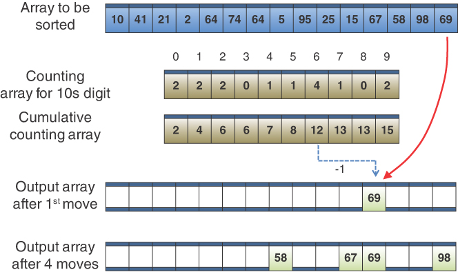
FIGURE 7-16 Applying the counting sort on the 10s digit
At the end of the loop, the counting array holds the number of matching keys for the different values of that particular digit. Some elements of the counting array may be zero, meaning that value of the digit did not appear in any key. A second loop through all but the first element of the counting array adds the count to the count on its left. That makes the rth element of the counting array contain the count of all keys that match r or less. In other words, it has the cumulative count of matching keys. The third row of Figure 7-16 shows the result of adding the counts. Note the final value in the array is always the total count of all the keys in the input.
The next step in the counting sort makes use of the cumulative counting array to move items from the input array to an output array. The process starts from the right (highest index) cell. In the data of Figure 7-16, the rightmost key is 69 and its 10s digit is a 6. The algorithm looks at the cumulative counting array at index 6, which is 12. That means there were 12 keys whose 10s digit was 6 or less. All those items must go in the first 12 cells of the output array. It decrements the count of the cumulative array at index 6 by 1. That is 11, and it moves the item from the input array, 69, into the output array at index 11.
The process repeats for each remaining item in the input array. The next one in Figure 7-16 is an item with a key of 98. It looks up 9 in the cumulative counting array, finds 15 stored there, decrements it to 14, and places the item at index 14 in the output, which is the final position. The third item to move is one with a key of 58, whose 10s digit is 5, so it is moved to index 7. When it gets to the fourth item to move, the key is 67. The 10s digit is 6, so it looks at index 6 in the cumulative counting array. This time it finds 11 there because it was decremented once before, so it decrements it again and places item 67 at index 10 of the output array. The last row of Figure 7-16 shows the state of the output array after moving the four items.
The counting sort “knows” where to put the items in the output array based on cumulative counting array values. These items are updated with each move so that every item goes to a unique position. After processing the 10s digit, the entire process would need to be repeated on the 100s digit of all the keys. That process would use the output array from the 10s digit process and put its results back in the input array. Of course, in this particular example, none of the keys has a nonzero hundreds digit, so it requrires only sorting by the 1s followed by the 10s digits. When all of the digits of all of the keys have been processed, the output array holds the sorted items. If there were an odd number of digits in the keys, one more copy operation would be needed to copy the result back to the input array.
The counting sort has the same complexity as the radix sort. Both run in O(N×log N) time and take O(N) memory. More precisely, both algorithms require O(N + R) memory and run in O(N × L), where R is the radix and L is the length of the keys, and L must generally be log N or greater. The difference is in what kind of structure is used for the intermediate results.
Timsort
In Chapter 3, you saw that the simple sorting algorithms could get O(N2) performance using O(1) memory. In Chapter 6, you saw that mergesort could get O(N×log N) performance using O(N) memory. Quicksort can get O(N×log N) performance using O(log N) memory in most cases but can degrade to O(N2) in some cases. Timsort is a balance between some of these extremes.
Tim Peters implemented Timsort for the Python sort() method in 2002 based on the mergesort, insertion sort, and some clever ideas to control the memory usage and guarantee O(N×log N) performance. Timsort uses half the memory that mergesort needs and has the side benefit of running in O(N) time on sorted input data, like the insertion sort. It is widely used outside of Python as well because of these characteristics.
Timsort is based around finding runs of items in the original array where the keys are either nondecreasing or strictly decreasing. The idea is to iterate over the items in the array until it finds a key that is lower than the key of its predecessor. That marks the end of a nondecreasing run and the beginning of a new decreasing run. Then it can look for the next key that is equal to or higher than its predecessor to find the end of the decreasing run. If it finds a decreasing run of two or more items, it swaps pairs of items from the ends like the quicksort partitioning algorithm to make it a nondecreasing run.
Figure 7-17 illustrates the runs that Timsort identifies. The height of each rectangle represents the key for that item. The array starts with an increasing sequence of four items. This group forms run 1, which is a nondecreasing run. The next four items form run 2, where the keys strictly decrease. After that, the next two items form run 3, which is nondecreasing. Adjacent keys with equal values are treated as nondecreasing, which leads to the next three runs being only two items each. Run 11 is one example where adjacent equal-valued keys are grouped together in the same run.

FIGURE 7-17 Runs in Timsort
The bottom panel of Figure 7-17 shows how Timsort reverses all the decreasing runs into nondecreasing ones. Now every run has nondecreasing key values.
It’s straightforward to create a generator that yields these runs as it walks along the sequence, converting any decreasing runs into nondecreasing runs, all in O(N) time. A loop in Timsort uses the generator to push the runs on a stack as they are produced. After adding a new run, it checks the conditions of the top three or four runs on the stack. Under certain conditions, it starts to combine the runs using mergesort. These collapse the small runs into bigger ones. Because the runs have keys that are nondecreasing, they are already sorted. Because it runs mergesort only on adjacent runs, the sorting can be done in place in the input array, leaving a larger sorted run where the two smaller runs were.
By mergesorting the top two runs on the stack repeatedly, the entire stack of runs could be sorted into a single run. Timsort uses several techniques to reduce the amount of extra space needed for those mergesorts. First, it can reduce subarray lengths by finding where in the first run the second run begins and only mergesorting the remainder of the first run. Likewise, items with keys higher than the last key of the first run can be excluded from the second run. When you use binary search, finding where these keys land in the sorted runs is quick, O(log N).
To keep memory down and maximize the efficiency, Timsort needs to balance the sizes of the runs that it merges. The merge algorithm needs temporary space for a copy of the smaller run, but not for the larger run. Figure 7-18 illustrates a case where runs K and K+1 within the larger input array have been selected for merging. First, Timsort identifies the left index, which is the first key higher than the lowest key in run K+1 (20). Similarly, the right index is the last key lower than the highest key in run K (59). Only the subarray between left and right needs to be merged because the other items in the full runs are already in their sorted positions.

FIGURE 7-18 Merging adjacent runs in Timsort
Knowing left, right, and the boundary index of the two runs, Timsort finds the length of the sub-runs that need to be merged. In the case shown in the figure, the higher sub-run is shorter, with only four cells. Those items must be copied to a temporary array, as shown in the lower part of the figure. That “empties” the cells in the input array to allow for a merge taking the highest key from the highlighted sub-runs and moving that item to the rightmost empty cell. If the lower sub-run were shorter, then the merge process would move the lowest keyed item into the empty cells at the left (lower) side. The merge process ends when all the items in the copied sub-run have been copied back to the input array.
Efficiency of Timsort
The Timsort algorithm is quite a bit more complex and intricate (perhaps even more beautiful) than quicksort and mergesort. We’ve left out some details, such as using the insertion sort to combine and sort short, adjacent runs and “galloping mode.” The benefit of all these techniques is that, overall, it has been shown to operate in O(N×log N) time, even in the worst case. In the best case of a forward- or reverse-sorted array, it runs in O(N) time. That extra speed comes at the cost of needing temporary storage for at most N/2 cells plus O(log N) storage for the stack of runs. In certain conditions, such as when the input data is already sorted, no merging of runs is needed, so the memory usage is O(1) in the best case. It ends up needing about half the memory of mergesort to cap the worst-case runtime, delivering the benefit of O(N) time for sorted data.
Summary
- The Shellsort applies the insertion sort to widely spaced elements of an array, then less widely spaced elements, and so on.
- The expression n-sorting means sorting every nth array element.
- A sequence of numbers, called the interval sequence, or gap sequence, is used to determine the sorting intervals in the Shellsort.
- A widely used interval sequence is generated by the recursive expression hi = 3 × hi–1 + 1, where the initial value, h0, is 1.
- If an array holding 1,000 items were first to be 364-sorted, then 121-sorted, then 40-sorted, then 13-sorted, then 4-sorted, and finally 1-sorted, it would be sorted more efficiently than by simply 1-sorting it.
- The Shellsort is hard to analyze, but runs in approximately O(N×(log N)2) time. This is much faster than the O(N2) algorithms like the insertion sort, but slower than the O(N×log N) algorithms like the quicksort and Timsort.
- To partition an array is to divide it into two subarrays, based on a key value of each item.
- The pivot value is the value that divides the other items during partitioning. Items with keys smaller than the pivot value go in the lower group; larger keyed items in the higher group.
- Items with keys equal to the pivot may go in either partition.
- Items in the lower partition have lower indices than those of the higher partition.
- In the partitioning algorithm, two array indices, each in its own
whileloop, start at opposite ends of the array and step toward each other, looking for items that need to be swapped. - When an array index points to an item that needs to be swapped, its
whileloop exits. - When both
whileloops exit and the indices have met or passed each other, the partition is complete. - When both
whileloops exit and the indices have not yet met, the items are swapped. - Partitioning operates in linear O(N) time, making N plus 1 or 2 comparisons and at most N/2 swaps.
- The partitioning algorithm may require extra tests in its inner
whileloops to prevent the indices running off the ends of the array. - Quicksort partitions an array and then calls itself twice recursively to sort the two resulting partitions (stored in subarrays).
- Subarrays of one or fewer elements are already sorted; this is the base case for quicksort.
- Quicksort uses the key value of a specific item in the subarray, called the pivot, to partition the subarry.
- In a simple version of quicksort, the pivot can be the item at the right end of the subarray.
- During the partitioning, the pivot is placed out of the way on the right and is not moved while the rest of the subarray is partitioned.
- Later the pivot is swapped into the space between the two partitions. This is its final sorted position.
- In the simple version of quicksort, performance is O(N2) for already sorted (or inversely sorted) data.
- An enhanced version of quicksort selects the pivot as the median of the first, middle, and last items in the subarray. This is called median-of-three partitioning.
- Median-of-three partitioning effectively eliminates the problem of O(N2) performance for already sorted data.
- In median-of-three partitioning, the first, middle, and last items are sorted at the same time the median is determined.
- This three-element sort eliminates the need for the end-of-array tests in the inner
whileloops of the partitioning algorithm. - Quicksort operates in O(N×log N) time (except in degenerate cases such as when the simpler version is applied to already-sorted data).
- Subarrays smaller than a certain size (the cutoff) can be sorted by a method other than quicksort.
- The insertion sort is commonly used to sort subarrays smaller than the cutoff.
- The radix sort is about as fast as quicksort but uses at least O(N) memory to store copies of the data.
- Generalized radix sort can be used to sort items whose keys are sequences of values, such as strings or tuples.
- The efficiency of a radix sort depends on how many values each sequence element can take, which is the radix value, and the maximum length of the key sequences.
- Timsort is a hybrid sorting technique that finds and merges runs in the input data.
- The runs in Timsort are adjacent items in the input array with either nondecreasing or decreasing key values.
- Timsort merges adjacent runs using an enhanced version of mergesort.
- Timsort runs in O(N×log N) time in the worst case and O(N) time for forward- or reverse-sorted input data.
- Timsort uses O(N) memory in the worst case.
Questions
These questions are intended as a self-test for readers. Answers may be found in Appendix C.
1. The Shellsort works by
a. partitioning the array into two parts.
b. swapping adjacent elements.
c. dealing with widely separated elements.
d. forming increasingly larger shells of elements that are already sorted.
2. If an array has 100 elements, then Knuth’s interval sequence algorithm would start with an interval of ________.
3. To transform the insertion sort into the Shellsort, which of the following do you not do?
a. Substitute h for 1.
b. Insert an algorithm for creating gaps of decreasing width.
c. Enclose the normal insertion sort in a loop.
d. Change the direction of the indices in the inner loop.
4. What could happen when using the Shellsort with an interval sequence created by repeatedly dividing the array size in half?
5. Fill in the Big O values: The speed of the Shellsort is more than _______ but less than ________.
6. Partitioning is
a. putting all elements larger than a certain value on one end of the array.
b. dividing an array into (almost) equal sized halves.
c. partially sorting parts of an array.
d. sorting each half of an array separately.
7. During partitioning, each array element is compared to the _______.
8. In partitioning, if an array element is equal to the answer to question 7,
a. it is passed over.
b. it is passed over or not, depending on the other array element.
c. it is placed next to the array element at the right end.
d. it is swapped.
9. True or False: In quicksort, the pivot can be an arbitrary element of the array.
10. Assuming larger keys on the right, the value returned by the __partition() method is
a. the element between the left and right subarrays.
b. the key value of the element between the left and right subarrays.
c. the index of the leftmost element in the right subarray.
d. the key value of the leftmost element in the right subarray.
11. Quicksort involves partitioning the original input array and then _________.
12. In the simple version of quicksort, after partitioning, the pivot may be
a. used to find the median of the array.
b. exchanged with an element of the right subarray.
c. used as the starting point of the next partition.
d. discarded.
13. Median-of-three partitioning is a way of choosing the _______.
14. In quicksort, for an array of N elements, the __partition() method will examine each element approximately ______ times.
15. What unfortunate outcome could happen when using quicksort and always choosing the rightmost element of subarrays as the input to the __partition() method?
16. True or False: You may speed up quicksort if you stop partitioning when the partition size is 5 or less and finish by using a different sort.
17. Radix sort
a. uses linked lists to hold elements whose keys have certain digits.
b. divides each element by 10 recursively to find its final sorted position.
c. first partitions the array in 10 parts, then rearranges elements in each partition by digits in their keys.
d. runs faster than quicksort because it doesn’t have to compare entire keys.
18. The memory needed for decimal radix sort of an array of N elements is O(_______).
19. The Timsort algorithm starts by
a. h-sorting the original array.
b. finding the median key of the input array.
c. merging the first and second halves of the array until keys start descending.
d. finding runs of elements with nondecreasing and decreasing keys.
20. What other sorting methods are used as part of Timsort?
a. Shellsort
b. mergesort
c. quicksort
d. h-sort
Experiments
Carrying out these experiments will help to provide insights into the topics covered in the chapter. No programming is involved.
7-A In the ShellSort() implementation of Listing 7-1, the number of shifts is counted and returned. Would adding a count of the number of key comparisons be helpful in measuring performance? If so, what would it show? If not, why not?
7-B Moving the pivot in quicksort by slicing the array and reinserting it between the subarrays as shown in Figure 7-8 would require a lot of copying of cells. Is there another data structure to use in place of the array that would allow slicing and splicing in constant—O(1)—time? If so, which one and why?
7-C The partitioning algorithm can put items with keys equal to that of the pivot in either partition. That means that using partitioning in a sort algorithm like quicksort cannot be stable. Try experimenting with partitioning arrays that have many duplicate keys. Using the AdvancedSorting Visualization tool, make a new array of 10 cells and fill it with random values. Delete the rightmost item five times to clear space. Then choose a value somewhere between the minimum and maximum, insert it five times, and shuffle the array. Before running the partitioning using the repeated key value, predict which partition each copy will end up in. Now run the partitioning to check your prediction. Reshuffle the array and try again. Can you generate a situation that demonstrates that the sort will not be stable? Can you generate an initial situation where the repeated key values are stable after the sort?
7-D Judicious choice of the pivot value speeds up the quicksort. Using the AdvancedSorting Visualization tool, make a new array of 10 cells and fill it with random values. Try to sort it using only a sequence of Partition operations where you choose the pivot. A very poor choice of the pivot might require 10 partitions to sort 10 items. How few partitions does it take you? Can you beat the quicksort? Of course, the initial ordering affects the number of partitions that will be needed. If the initial order happens to be increasing order, you don’t need any partitioning. You can always get the same order of 10 items by restarting the Visualization tool.
7-E Consider using the quicksort algorithm to rank order teams in a tournament. One team is chosen at random as the “pivot” team. It plays each of the other N–1 teams. The teams that beat the pivot team go into bracket A and those that lose go into bracket B. Teams that tie the pivot team would go into alternating brackets (first A, then B, then A, then B). The pivot team is then placed into the bracket with the fewest teams. Then each bracket conducts its own rank ordering using the same algorithm except that the choice of the pivot team for a bracket must be a team with the fewest number of previous selections as pivot within that bracket. The brackets would get smaller with each iteration until they reach size 1, and the sequence of bracket placements would determine the overall ranking of a team with A-A-A-A being highest, B-B-B-B being lowest, A-B-B-B being in the middle, and so on.
How many games would take place for a whole tournament of 16 teams? How many games would each team play? How does that compare with other tournament competition ladders that you’re familiar with? If the exact numbers of games is variable or hard to determine, find the best and worst case numbers.
Programming Projects
Writing programs to solve the Programming Projects helps to solidify your understanding of the material and demonstrates how the chapter’s concepts are applied. (As noted in the Introduction, qualified instructors may obtain completed solutions to the Programming Projects on the publisher’s website.)
7.1 Extend the ShellSort.py module of Listing 7-1 to include the two other interval sequences described in the text, namely dividing the interval by 2.2 and truncating, and Flamig’s formula. For both methods the first interval, h, should be calculated as if the preceding value of h was the number of array elements. Set up a program that creates an input array and passes copies of that array to the three Shellsort methods (Knuth’s sequence, divide by 2.2, and Flamig’s sequence). Compare the number of shifts performed on (a) an array that is already sorted, (b) an array that is inversely sorted, and (c) a random ordering. Use a loop to perform the test with arrays of length 95 to 100 elements. Is there a method that clearly performs fewer shifts?
7.2 Modify the quicksort() and helper methods in Listings 7-7 and 7-8 to count the number of item copies and key comparisons they make during a sort and return the counts to the caller (using Python’s ability to return multiple values). For the copies, a swap counts as 3 copies. For the comparisons, only count comparisons of key values (not array indices). Use the modified method to show how many copies and comparisons are made when sorting (a) a forward-sorted array of 50 items, (b) a reverse-sorted array of 50 items, (c) a constant value for all 50 items, and (d) an array of 50 random items. For each of those array styles, show the counts when short is 3, 7, and 11 to see the effect of using insertion sort for the shorter subarrays. Use the same random array for all variations of the short parameter to make a fair comparison.
7.3 In Exercise 3.2 in Chapter 3, we suggested finding the median of a set of data by sorting the data and picking the middle element. You might think using quicksort and picking the middle element would be the fastest way to find the median, but there’s an even faster way. The quickselect algorithm uses partitioning to find the median without completely sorting the data.
To see how this works, imagine that you partition the data choosing the rightmost item as the pivot, and, by chance, the pivot happens to end up at the middle element. You’re done! All the items to the right of the pivot are larger (or equal), and all the items to the left are smaller (or equal), so if the pivot falls in the exact center of the array, then it’s the median. The pivot won’t end up in the center very often, but you can end up getting the median by solving a smaller problem: repartitioning the partition that contains the middle element.
Suppose your array has seven elements numbered from 0 to 6. The middle is the element at index 3. If you partition this array and the pivot ends up at 4, then you need to partition again from 0 to 4 (the partition that contains index 3), not 5 to 6. If the next pivot ends up at 2, you need to partition from 2 to 6, not 0 to 1. You continue partitioning the appropriate parts recursively, always checking if the pivot falls on the original middle element at index 3. Eventually, it will, and you’re done. Because you need fewer partitions than in quicksort, this algorithm is faster.
The quickselect algorithm generalizes the goal a little more by letting the caller ask for any index in the subarray. So, for example, if you wanted the 90th item among an array of 100 numbers, you would call quickselect() with a goal index of 90 (or maybe 89, depending on what exactly is needed). If you choose 90, quickselect() would return whatever item would get sorted into the cell at that index by quicksort(), while only partially sorting the array. To get the median, the goal index would be 50 for the 100-element array. Extend your solution to Programming Project 7.2 to implement the quickselect() method and make another method, median(), to get the middle element of an array. Your implementation should make recursive calls somewhat like those in quicksort, but they will only partition each subarray, not completely sort it. Use the rightmost element of the subarray as the pivot, as was done in qsort(). The process stops when the goal index is found, not when the array is sorted. As an extension of Programming Project 7.2, your method should also return the number of copies and comparisons made. Use your method to show the median found, the number of copies, and the number of comparisons for the same kinds of inputs as the previous project, namely, (a) a forward-sorted array of 50 items, (b) a reverse-sorted array of 50 items, (c) a constant value for all 50 items, and (d) an array of 50 random items.
7.4 Implement a decimal radix sort for arrays as described in the “Designing a Radix Sort Program” section. It should handle variable amounts of data and variable numbers of digits in the key. You could make the radix a parameter as well (so it can be something other than 10), but it will be hard to see what’s happening unless you develop a routine to print values in different bases. Count the number of item copies made by the program. Show the results for arrays of 50 items whose maximum key is 99 and 999 to see the differences key length makes. Your program will need to determine how many digits are in the keys by examining the inputs and the radix (typically as the first pass through all the items is completed).
7.5 Implement a simplified version of the Timsort algorithm described in the “Timsort” section. Specifically, make a generator that looks for runs in an input array that are either nondecreasing or decreasing. The generator should reverse decreasing runs into increasing runs before it yields the lo, hi index pair that represents the run. Write a mergerun() method that takes two adjacent runs in the input array, uses a binary search to find the positions within the runs that need to be merged, copies the shorter section to a temporary array or other structure, and then merges the items back into the input array. The Timsort() method should use the generator to identify runs, one at a time, merging the second run into the first until the entire array is sorted. Show the program working on (a) a forward-sorted array of 50 items, (b) a reverse-sorted array of 50 items, (c) a constant value for all 50 items, and (d) an array of 50 random items.