
Chapter 12
Spatial Data Structures
In This Chapter
So far, all our data structures have stored records containing a key to identify them. That’s perfect when you want to find a record that exactly matches a key. What about when you want to identify items by position—for example, finding all the grocery stores within a certain distance of a particular location? For that task, you need a structure that uses two separate numeric keys to identify the location of records that correspond to points in space.
Although this pair of numbers may seem to be a simple extension from one numeric key, the data structures must be dramatically changed to make the kinds of desired operations happen efficiently. The nature of points in space and their distances drives much of the design. We look first at the ways to represent points in space and then at three ways of storing records associated with those points. We wrap up with a discussion of the performance that you can expect from these structures and some extensions needed for other domains.
Spatial Data
Data that has position attributes is called spatial data. Spatial data includes Cartesian coordinates and geographic coordinates.
Cartesian Coordinates
The simplest form of spatial data corresponds to points on a flat surface. Each point is represented by a pair of numbers that specify its X and Y coordinates on the surface, usually written as (x, y). These (x, y) coordinates on a flat surface are known as Cartesian coordinates, invented by French mathematician René Descartes. For example, if you were programming a simulation of a football game, you could use Cartesian coordinates to represent the location of each player on the field. Because a football field is a very small piece of the surface of the Earth, you can conveniently pretend that the surface of the field is perfectly flat, so it is appropriate to use Cartesian coordinates.
Cartesian coordinates could be represented using any convenient unit of distance—for example, pixels on a screen, or feet or meters on a playing field. The exact units chosen are important to the application but do not affect the data structures and algorithms if the units are the same for both dimensions.
Geographic Coordinates
Spatial data points on the surface of the Earth are usually represented by a pair of numbers that specify the latitude (the angle north or south from the equator) and the longitude (the angle east or west from the prime meridian at Greenwich, England). Some applications also require a third value corresponding to the elevation on or above the surface of the Earth. In this chapter, we consider just points that are on the surface of the Earth, that is, at sea level.
Figure 12-1 shows how the globe is divided into hemispheres by the equator in blue and the prime meridian in red. For example, the location of Ottawa, Canada, is approximately (45.30096°, –75.81689°) as shown by the small green dot. The negative longitude indicates that the point is to the west of the prime meridian. The location of Johannesburg, South Africa, is about (–26.17643°, 28.04551°) marked by another dot. The negative latitude indicates that Johannesburg is south of the equator. Latitude, longitude coordinates are known as geographic coordinates.
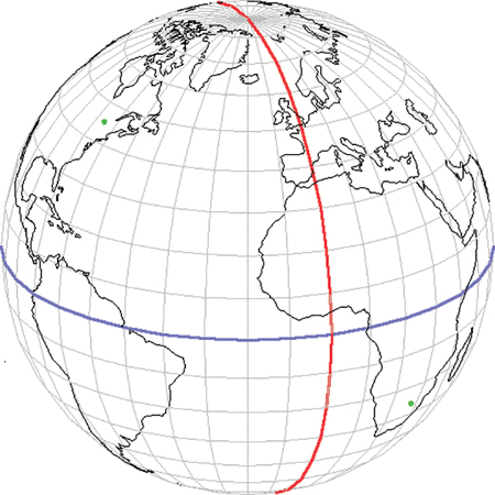
FIGURE 12-1 Geographic coordinates use longitude and latitude
Computing Distances Between Points
Later in this chapter, we look at data structures that support searching for records at or near specified Cartesian or geographic coordinates. To do these calculations, you need to be able to compute the distance between two spatial data points. This calculation is easy to implement for Cartesian coordinates and a little more complicated for geographic coordinates.
Distance Between Cartesian Coordinates
To compute the distance between two points specified by Cartesian coordinates, you make use of the familiar Pythagorean theorem that the length of the hypotenuse squared is the sum of the squares of the sides of a right triangle. Because the points are defined by their coordinates in the X and Y axes, you can align a right triangle with the axes to determine what is sometimes called the Euclidean distance. If the two points are at (x1, y1) and (x2, y2), then the Euclidean distance d between the two points is
Implementing this distance measure is simple in Python, as shown in Listing 12-1. The result of this formula is in the same units of measurement as the input Cartesian coordinates.
LISTING 12-1 Euclidean Distance Between Cartesian Coordinates
# return the Euclidean distance between points (x1,y1) and (x2,y2)
def euclideanDistance(x1, y1, x2, y2):
    dx = x2 – x1
    dy = y2 – y1
    return (dx*dx + dy*dy) ** 0.5
Distance Between Geographic Coordinates
Calculating the distance between geographic coordinates is more complex. First, geographic coordinates are specified as angles of latitude and longitude on the Earth—which do not directly correspond to distances expressed in units of length. Second, the surface of the Earth is neither flat nor perfectly spherical, which further complicates the computation. There are many ways that distance between geographic coordinates can be calculated. The accuracy of the calculations depends on the simplifying assumptions and approximations used.
The shortest path between two points on a sphere lies along the curve of a great circle. To get the great circle, take the plane that contains the two points and the center of the sphere and intersect it with the sphere itself. Computing the distance between Ottawa and Johannesburg using the Euclidean distance would be useful only if you could travel in a straight line through the Earth. Even a straight line drawn on Figure 12-1 that seems to go directly between the two points is not necessarily the shortest path. To be sure that the path is the shortest, it must lie on the great circle path that connects them. That is why a flight from New York to Spain flies in a path that curves toward the North Pole, rather than flying due east, as a typical map might imply.
The haversine formula computes the great circle distance between two geographic coordinates on a sphere. Although Earth is not a perfect sphere, the haversine formula will give correct answers to within 0.5 percent. That should be adequate for finding the nearest airport or coffee shop, but possibly not accurate enough for other applications. The haversine formula for the distance between two geographic coordinates is
where
 R is the radius of the Earth
-
-
-
Although this formula looks rather daunting, the Python implementation is straightforward, as shown in Listing 12-2.
LISTING 12-2 Python Implementation of the Haversine Distance
from math import *
RADIUS_OF_EARTH = 6371      # radius in kilometers

# return the haversine distance between (lon1, lat1) and (lon2, lat2)
def haversineDistance(lon1, lat1, lon2, lat2):
    lat1 = radians(lat1)    # trig functions need radians
    lon1 = radians(lon1)
    lat2 = radians(lat2)
    lon2 = radians(lon2)

    dLon = lon2 - lon1      # difference of longitudes
    dLat = lat2 - lat1      # difference of latitudes
                            # Haversine formula:
    a = sin(dLat/2)**2
    if dLon != 0:           # save some trig for dLon == 0
        a += cos(lat1) * cos(lat2) * sin(dLon/2)**2

    # Numerical issues at antipodal points requires min, max:
    return 2 * RADIUS_OF_EARTH * asin(min(1, max(a, 0)**0.5))
It is worth noting that as commonly spoken in English, geographic coordinates are referred to as “latitude, longitude” pairs. When you’re writing code to uniformly support either Cartesian or geographic coordinates, however, it makes more sense to refer to geographic coordinates as “longitude, latitude” pairs. Simply put, longitude angles correspond to values along the equator, analogous to points along the Cartesian X axis. Likewise, latitude angles correspond to values along the north-south meridians, analogous to the Cartesian Y axis. The methods in the class definitions we present for spatial data structures accept “a, b” pairs to specify spatial location, which are then interpreted appropriately to mean either x, y or longitude, latitude coordinates. Although the Euclidean distance will work with any units, this definition of the haversine distance always returns the distance in kilometers because the Earth’s radius is specified that way.
Circles and Bounding Boxes
When working with spatial data, you frequently need to determine whether points lie within a particular area. For example, you might want to know whether a particular geographic coordinate lies within a particular country or within a property boundary. Many kinds of regions might be checked. The two simplest and most common ones are circular and box-shaped areas. You will need to use the distance calculations in many cases to determine whether a point is inside or outside one of these regions.
Clarifying Distances and Circles
When you begin the search for a data point nearest to a query point, and no data point has been considered yet, it is convenient to think of the initial distance from the query point to the nearest point as being at infinity—in other words, a number that is arbitrarily large. The Python math module conveniently provides a predefined constant math.inf, which is larger than any other int or float number. (In versions of Python before 3.5, the constant for infinity was produced by the expression float('inf'), which can still be used.) As the search proceeds, and subsequent points are encountered, that distance becomes a finite number, which gets successively smaller as points closer to the query point are identified.
In Cartesian coordinates, at any step of the search, you can think of the query point together with the distance to the nearest point so far as defining a circle around the query point, whose radius is equal to the distance to the current nearest point.
In geographic coordinates, a curve of constant distance is not a perfect circle when drawn on a grid whose latitude lines and longitude lines are spaced at uniform degrees of separation (known as the Mercator projection). Indeed, this is what causes the apparent distortion of landmasses when viewed on some maps. For example, near the poles, the meridians are much closer together than they are near the equator.
These changes in distance are illustrated in Figure 12-2 where three 1,000 km paths have been drawn in blue. The same paths are drawn on the globe as it appears from space and on a map using the Mercator projection with 10 degrees separating each of the longitude and latitude grid lines. The path around Iceland looks much larger than the path centered on the coast of Brazil in the Mercator projection, even though both are equal diameter. The path surrounding the tip of Tierra del Fuego, the southern tip of South America (only partially visible on the globe projection), is also the same diameter.

FIGURE 12-2 Comparing 1000 km circles at different points on the globe
In the following pages when we discuss a query circle, keep in mind that sometimes the circle is not truly circular. The term query circle is used to refer to a curve of constant distance from a query point, which may not always look perfectly circular depending on the map viewpoint. Our computations account for this apparent distortion.
Bounding Boxes
As we just mentioned, when using geographic coordinates, a query circle with a radius of constant distance does not look like a circle when projected on a map grid with uniform latitude and longitude spacing. For geographic coordinate query circles far from the equator, the circle begins to look more like an ellipsoid. In addition, the widest part of the query circle is not directly due-east or due-west of the center of the query circle as it is at the equator or in Cartesian coordinates. For example, as a search circle gets farther north from the equator, the circle gets increasingly flattened, and the widest part of the search circle progresses farther north of the center of the circle.
In the coming pages we examine data structures that partition space into rectangular pieces. To search for a particular point, the algorithms repeatedly check whether a query circle intersects a particular rectangular piece of space containing data points. It can be computationally complex to determine whether a circle and rectangle intersect, and, even more so, whether a distorted ellipsoid and a rectangle intersect.
One way to simplify these repeated query circle-rectangle intersection calculations is to approximate the query circle by a rectangular bounding box that snugly encloses the query circle in either Cartesian or geographic coordinates. As you will see, determining whether two rectangles intersect is a fast and simple computation. If the bounding box of the query circle doesn’t intersect a rectangle of space, then you can be certain that there’s no chance that the query circle itself intersects the rectangle of space. Only when the bounding box does intersect a rectangle of space do you need to do more detailed calculations to attempt to find a point within that rectangle that matches or is nearby the query point.
The Bounding Box of a Query Circle in Cartesian Coordinates
In Cartesian coordinates, you can easily identify the left, right, top, and bottom coordinates of the bounds of a query circle of radius r, with a center at a, b, as shown in Figure 12-3. The left boundary lies at a – r. The right boundary lies at a + r. The vertical boundaries are similar.
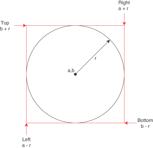
FIGURE 12-3 The bounding box of a circle in Cartesian coordinates
The Bounding Box of a Query Circle in Geographic Coordinates
How do you determine the bounding box of a query circle of radius r in geographic coordinates? It’s clear that you need to calculate the bounds for longitude and latitude, but how? The formulas that solve this problem (shown here) employ methods in spherical geometry that are outside the scope of this text.
You do not need to understand the detailed math to create the methods that compute and use the bounding box of a search circle in geographic coordinates. The preceding equations and the diagram in Figure 12-4 show how to compute the width in longitude and height in latitude from the center of the query circle to the edges of its bounding box, where
- r is the radius of the query circle.
- R is the radius of the Earth.
- B is the latitude b of the a, b center of the query circle, expressed in radians instead of degrees.
- (Δlong) is the longitude width in radians from the center to the widest point of the query circle.
- (Δlat) is the latitude height in radians from the center to the top or bottom of the query circle.

FIGURE 12-4 The bounding box of a query circle in geographic coordinates
Note that the widest point of the query circle may not be due east of the center. The example shown in the figure illustrates this distortion resulting in the widest part of the circle being slightly vertically offset from the latitude, b.
Implementing Bounding Boxes in Python
We represent bounding boxes of all types in Python using the Bounds class and its CircleBounds subclass, as shown in Listing 12-3.
LISTING 12-3 Creating and Adjusting Bounds Objects
class Bounds(object):
    def __init__(self, left = -inf, right  = inf,
                       top  =  inf, bottom = -inf):
        Bounds.adjust(self, left, right, top, bottom)

    # mutator to initialize/change bounds in existing object
    def adjust(self, left, right, top, bottom):
        self.__l = left
        self.__r = right
        self.__t = top
        self.__b = bottom

    # return a new Bounds, where some of the
    # current boundaries have been adjusted
    def adjusted(self, left = None, right = None,
                       top = None,  bottom = None):

        if left   == None: left   = self.__l
        if right  == None: right  = self.__r
        if top    == None: top    = self.__t
        if bottom == None: bottom = self.__b

        return Bounds(left, right, top, bottom)
Instances of the Bounds class shown in Listing 12-3 store the coordinates of the left, right, top, and bottom boundaries of a rectangular section of Cartesian or geographic space. You can create a new Bounds object by invoking the constructor as shown in this snippet:
b = Bounds(-125.6, -60.8, 49.72, 23.77)
The returned object represents the rough rectangular boundaries of the continental United States, with its left boundary at –125.6 degrees longitude, its right boundary at –60.8 degrees longitude, its top boundary at 49.72 degrees latitude, and its bottom boundary at 23.77 degrees latitude.
Invoking Bounds() with no arguments results in a rectangle with infinite extent. The mutator method, adjust(), enables the client code and the constructor to update the private attributes.
A separate method called adjusted() creates and returns a new Bounds object derived from the current object, and with some or all the boundaries replaced with new values.
The CircleBounds Subclass
The CircleBounds subclass of Bounds, shown in Listing 12-4, creates a box enclosing a circle.
LISTING 12-4 Initializing and Adjusting CircleBounds objects
# A bounding box that surrounds a search circle. Properly handles
# distorted circles resulting from geographic coordinates.
class CircleBounds(Bounds):
    # create the bounding box that surrounds the search
    # circle at a,b,r using the specified distance function
    def __init__(self, a, b, r, func):
        # remember the circle's parameters for later
        self.__a, self.__b, self.__r = a, b, r
        self.__func = func

        # get the width/height of the bounding box
        deltaA, deltaB = self.__deltas(a, b, r, func)

        # initialize the superclass's rectangular bounds
        super().__init__(a - deltaA,         # left
                         a + deltaA,         # right
                         b + deltaB,         # top
                         b - deltaB)         # bottom

    # if the circle's radius changed, mutate its bounds
    def adjust(self, r):
        if r != self.__r:
            self.__r = r

            # new dimensions of bounding box
            deltaA, deltaB = self.__deltas(
                self.__a, self.__b, r, self.__func)

            # update the box
            super().adjust(self.__a - deltaA,  # left
                           self.__a + deltaA,  # right
                           self.__b + deltaB,  # top
                           self.__b - deltaB)  # bottom
The user creates a new CircleBounds object by invoking the constructor with the a, b coordinates of a circle center, the circle’s radius, and a reference to a distance function, as shown in this snippet:
c = CircleBounds(38.736, -9.142, 3.14, haversineDistance)
This snippet creates a CircleBounds object that represents the rectangular bounds surrounding a circle centered in Lisbon, Portugal, with a radius of 3.14 km.
As shown in Listing 12-4, the constructor saves the parameters in private attributes—to potentially be used later by the adjust() mutator method that adjusts the radius of the circle. Given the a, b coordinates and radius r of the circle, the constructor obtains the distances from the center of the circle to the widest and tallest points on the circle, called deltaA and deltaB. Finally, the constructor uses those two distances to invoke the superclass’s constructor with the rectangular bounds of the circle.
The adjust() mutator can be invoked by the client with a new value for the circle’s radius. If adjust() determines that the radius has changed, then deltaA and deltaB are recomputed, and then the superclass’s adjust() method replaces the rectangular bounds with the newly computed boundaries.
All that remains to discuss is how the deltaA and deltaB distances are computed, as shown in the __deltas() method in Listing 12-5. The method implements the calculations for width and height of the two types of circles shown in Figure 12-3 and Figure 12-4. For infinite radius circles or Cartesian coordinates, deltaA and deltaB are simply the radius of the search circle. For geographic coordinates, deltaA and deltaB are computed using the preceding complex formulas and substituted for Δlong and Δlat in Figure 12-4, respectively.
LISTING 12-5 Computing the Width and Height of a Bounding Box Around a Circle
class CircleBounds(Bounds):
…

    def __deltas(self, a, b, r, func):
                # When r is infinity, bounds are always infinite
                # For cartesian coordinates, the edges of the bounding
                # box are r away from the center of the search circle.
        if r == inf or func == euclideanDistance:
            deltaA = deltaB = r

        else:   # geographic coordinates
                # The width of the bounding box is determined by
                # the width of the distorted circle at its widest point.
            alpha = r / RADIUS_OF_EARTH
            gamma = radians(90 - abs(b)) # b is latitude

                # if the circle itself crosses the pole then
                # alpha >= gamma, so we set deltaA as inf,
                # effectively treating the width as if it were inf
            if alpha >= gamma:
                deltaA = inf

            else:
                # the circle doesn't cross a pole, so get
                # longitude angle from center of circle at
                # the circle's widest width calculated using
                # a spherical right triangle identity.
                deltaA = degrees(asin(sin(alpha) / sin(gamma)))

                # latitude angle directly above/below the
                # center of the circle. This works since above
                # or below is directly on a meridian.
            deltaB = degrees(alpha)

        return deltaA, deltaB
Recall that for geographic coordinates, a query circle gets progressively flattened as it approaches either pole. If the center of the circle gets within the query radius of a pole, the circle extends beyond the pole (in other words, the pole lies within the query circle). This condition is detected in the code when the alpha variable exceeds the gamma variable, which could result in an undefined value of the inverse sine function used to compute deltaA. In that case, instead of computing the inverse sine, it sets deltaA to be infinite because the search circle wraps all the way around the pole.
Determining Whether Two Bounds Objects Intersect
Later in this chapter in the discussion of the Grid and QuadTree classes, some methods need to determine whether two rectangles defined by their Bounds objects intersect. You can determine whether two rectangles intersect by making the simple observation that they do not intersect if one rectangle is fully to the left of the other or fully above the other.
As illustrated in Figure 12-5, rectangles 2, 3, and 4 do not intersect with rectangle 1 because they are each either directly above or to the side of rectangle 1. Rectangle 5, however, does intersect with rectangle 1.
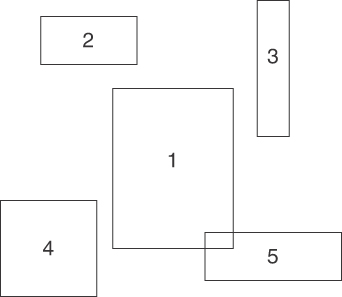
FIGURE 12-5 Intersecting and nonintersecting rectangles
For any two rectangles A and B, you can say that they don't intersect if the following pseudocode expression is true:
(A is to the left of B) or (B is to the left of A) or
(A is above B) or (B is above A)
So, to determine whether rectangles A and B do intersect, you simply negate that entire expression and simplify, resulting in
(A is NOT to the left of B) and (B is NOT to the left of A) and
(A is NOT above B) and (B is NOT above A)
Examining rectangles 1 and 5, you can see that this latter expression evaluates to True, and therefore that rectangles 1 and 5 do intersect.
The code in Listing 12-6 shows the simple implementation of the intersects() method. It uses the negation of the definition of not intersecting.
LISTING 12-6 Determining if Bounds Objects Intersect
class Bounds(object):
…
            # return True if bounds of the rectangles intersect.
            # Two rectangles don't intersect if one is totally to
            # the left of or above the other. So we negate to
            # determine if they do intersect.
    def intersects(self, other):
        return not (
            # check if self's box is to left or right of other
            self.__r < other.__l  or  self.__l > other.__r or

            # check if self's box is above or below other
            self.__b > other.__t  or  self.__t < other.__b)
Determining Whether One Bounds Object Lies Entirely Within Another
As you will soon see, some methods also need to determine whether the bounds of a circle fit entirely within the bounds of a square subset of cells on a grid.
Figure 12-6 illustrates a sample scenario, where you want to determine whether the circle drawn in black, with its bounding box drawn in red, lies entirely within the blue-shaded square of grid cells. If you have a Bounds object initialized with the boundaries of the blue shaded area, and another CircleBounds object initialized with the bounding box surrounding the circle, it is simple to determine whether the circle fits within the blue box, as shown in the within() method in Listing 12-7.

FIGURE 12-6 A CircleBounds within another Bounds object
LISTING 12-7 Determining Whether a Bounds Object Lies Within Another Bounds Object
class Bounds(object):
…
    # return True if the bounds of self fall within other
    def within(self, other):
        return (self.__r < other.__r and
                self.__l > other.__l and
                self.__t < other.__t and
                self.__b > other.__b)
Note that the same definition of within() is used for both Bounds and CircleBounds objects. This is good enough for the purpose of searching the data structures but would not correctly determine whether the circle of one CircleBounds object was truly within (or even overlapping) the circle of another CircleBounds object.
Searching Spatial Data
Now that we’ve handled these geometry basics, we can focus on the interesting challenge of searching a collection of spatial data points to find an exact match to a query point or to find the closest match to a query point. To find the closest match, we need to specify what it means to be close; in other words, which distance function should be used to compare a query point to a candidate data point? If the spatial data consists of Cartesian coordinates, the euclideanDistance() function will be appropriate. If the spatial data consists of geographic coordinates, the haversineDistance() function will be appropriate.
In the following sections, we look at several classes that implement data structures and algorithms to support exact match and closest match spatial search. The classes vary in code complexity and Big O performance, so their applicability depends on the amount and distribution of data you are attempting to process. The important issues are how to deal with using coordinates as keys and how to deal with distance when searching. First, we start with a simple approach. Then we add more complex structures to improve performance. Finally, we look at the trade-offs between the different approaches.
Lists of Points
If you want to support spatial data search of a small number of points, it can be appropriate to just store the spatial data points in one of the structures you’ve already seen, such as an array or a list. Then the spatial data is queried by traversing over the items to find either an exact match or the closest match to the query point. This brute-force approach is the simplest possible solution, though because of that simplicity, the Big O performance is O(N) to search for an exact or nearest match. In other words, to do a spatial search using brute force, the code must compare the query point to every point stored in the structure.
Creating an Instance of the PointList Class
We’ll use a simple Python list (array) to hold a collection of items in a PointList class. Client code creates an instance of the PointList class by invoking the constructor to create an object that contains Cartesian points:
b = PointList('cartesian')or that contains geographic points:
b = PointList('geographic')If the constructor is passed any string other than 'cartesian' or 'geographic', an exception will be raised.
LISTING 12-8 The PointList Constructor
class PointList(object):
    def __init__(self, kind):     # must specify type of coordinate
        if kind == 'cartesian':
            self.__distance = euclideanDistance
        elif kind == 'geographic':
            self.__distance = haversineDistance
        else:
            raise Exception("Invalid kind of coordinate")

        self.__points = [ ]       # keep track of inserted points
Listing 12-8 shows the code for the PointList constructor. There are just two private attributes: a reference to the distance function appropriate to either Cartesian or geographic coordinates, and a reference to an initially empty list that will be used to store the points in the object.
Inserting Points
Points are inserted into the PointList object using the insert() method. For Cartesian points, the user passes to the insert() method an x coordinate, a y coordinate, and a reference to whatever data will be associated with the Cartesian x, y point:
b.insert(34, 56, "Player 1") # insert a point at x == 34, y == 56Likewise, for geographic points, the user passes to insert a longitude, a latitude, and a reference to the data associated with this geographic longitude, latitude point:
b.insert(-73.987853, 40.748440, "Empire State Building")
Most likely, the client code will use a loop to repeatedly invoke insert() so that the PointList object contains all the points to be searched.
The implementation of the PointList.insert() method is quite simple (see Listing 12-9). Each inserted point is stored as a tuple containing three elements appended to the end of the private __points list. Each tuple contains
- The x, or longitude, coordinate
- The y, or latitude, coordinate
- A reference to the data to be associated with the specified point
LISTING 12-9 Inserting a Point into a PointList
class PointList(object):
…
    def insert(self, a, b, data):
        # Loop through the points looking for an exact match
        for i in range(len(self.__points)):
            p = self.__points[i]
            if p[0] == a and p[1] == b:         # Replace data
                self.__points[i] = (a, b, data) # for a duplicate
                return

        self.__points.append((a, b, data))      # not there, so append
For all the data structures in this chapter, the insert() method ensures that there are no points stored with duplicate a, b coordinates. Thus, for PointList, insert() loops through all the points in the list, and if it finds an already-existing point with the same a, b coordinates, the data currently stored for that point is replaced with the newly inserted data. If no duplicate is found, then the insertion is accomplished by appending a point to the end of the __points list. When the client later attempts to find an exact or nearest match, the findExact() or findNearest() methods will return the single point that is found to match the query point, and the returned data will be the data that had been most recently inserted for those coordinates. Because insert() loops over all the points in the list to avoid inserting a point with duplicate coordinates, it takes O(N) time for each insertion.
Finding an Exact Match
You call the findExact() method to search for the point contained in the PointList object that exactly matches the specified x, y or longitude, latitude coordinates. If an exact match is found, the method returns a reference to the data that was stored for the matching point:
>>> ans = b.findExact(-73.987853, 40.748440)
>>> print("Answer was:", ans) # Answer was: Empire State Building
Not surprisingly, the implementation of findExact() shown in Listing 12-10 is simple. The method loops through potentially every point stored in the __points list. If an exact match to the specified a, b coordinates is found, then the data for that point is returned to the client.
LISTING 12-10 Finding an Exact Match in a PointList
class PointList(object):
…
    def findExact(self, a, b):          # Return data for exact point
        for p in self.__points:         # Loop through all points
            if p[0] == a and p[1] == b: # found exact match
                return p[2]             # so return its data
        return None                     # Couldn't find a match!
Because findExact must potentially loop through every point of the __points list in the worst case, the complexity of the method must be O(N).
Deleting a Point
It is straightforward to implement a method to delete from the PointList a point specified by a pair of coordinates. As shown in Listing 12-11, the approach is very similar to that used by findExact(), except that after the matching point is identified, it is removed from the list using Python’s del operator. If a matching point is found, then delete() returns the data associated with the deleted point. Otherwise, delete() returns None.
LISTING 12-11 Deleting a Point from a PointList
class PointList(object):
…
    # delete the point at a,b
    # Return the deleted point's data if found, or None
    def delete(self, a, b):
        # Loop through the points looking for an exact match
        for i in range(len(self.__points)):
            p = self.__points[i]
            if p[0] == a and p[1] == b: # found a match
                del self.__points[i]    # delete the point
                return p[2]             # return its data

        return None                     # point wasn't there
Just like findExact(), the Big O time for delete() is O(N).
Traversing the Points
Because PointList is implemented as a simple list of tuples, traversing the points is trivial. As with the other data structures you’ve seen, traverse() is implemented as a generator as shown in Listing 12-12.
LISTING 12-12 The traverse() method of PointList
class PointList(object):
…
    def traverse(self):
        for p in self.__points:         # yield each of the tuples
            yield p
The implementation loops through each of the elements of the list, yielding the tuples containing the a, b coordinates and the associated data. Because every point in the list is visited once, the complexity of traverse is O(N). The caller can use tuple-assignment in its for loop to assign the values to three variables, or just assign the returned tuple to a single loop variable.
Finding the Nearest Match
You call the findNearest() method to find the point stored in the __points list that lies closest to the query point. Depending on whether the PointList object stores Cartesian or geographic coordinates, findNearest() automatically uses the appropriate function to compute the distance from the query point to each of the object’s points, as shown in Listing 12-13.
LISTING 12-13 Finding the Nearest Point in a PointList
class PointList(object):
…
    def findNearest(self, a, b):     # find closest point to (a,b)
        if len(self.__points) == 0:  # No points yet?
            return None

        distance = inf               # Assume no nearest point
        for p in self.__points:      # For each point
            newDist = self.__distance(a, b, p[0], p[1])
            if newDist == 0:         # Nothing could be closer!
                return p[0], p[1], p[2], 0
            if newDist < distance:   # If it is closest so far,
                distance = newDist   # remember the distance,
                answer   = p         # and the point

        return answer[0], answer[1], answer[2], distance
The method returns to the client a four-element tuple containing the x/longitude, y/latitude, the associated data, as well as the distance to the point that is closest to the query point. The distance function that was set when the object was constructed determines the units of the measurement.
For example, assuming that a geographic point for the location of the Eiffel Tower has already been inserted in the PointList object, this snippet shows what would be returned by an invocation of findNearest():
>>> ans = b.findNearest(2.2, 48.8)
>>> print(ans)  # (2.294694, 48.858093, 'Eiffel Tower', 9.47495437535)
The implementation of findNearest() shown in Listing 12-13 starts by checking the base case of an empty list. If the PointList is empty, there is no nearest point, so None is returned. If there are some points, it initializes the distance variable to infinity and then loops through all the points. If the distance from a, b to one of the new points is less than the current best distance, it updates the answer and then records the new best distance.
This approach is not efficient because it is necessary to compute the distance between the query coordinates and every point stored in the PointList object’s __points list. The only shortcut happens when the query point has the exact same coordinates as one of the points in the __points list, in which case there would be no reason to keep looping through the remaining points and it returns the current point as the answer. The complexity of findNearest() is also O(N) for each invocation.
Grids
The PointList class is appropriate to store and query only a relatively small number of spatial data points. If you have many points and they are mostly uniformly spread out in space, then you can superimpose a grid on top of the points to speed up the insert(), findExact(), and findNearest() methods. To see why this is so, consider Figure 12-7, which shows a collection of 2,000 spatial data points, with a query point shown as a red diamond.

FIGURE 12-7 Two thousand data points and a query point
.To find a point that exactly matches or is closest to the red query point, every one of the 2,000 points must be compared to the red query point. If you superimpose a grid on top of the points, you can break them up into 10 rows and 10 columns of cells, as in Figure 12-8.

FIGURE 12-8 Breaking up space into a 10 × 10 grid
To find whether there’s an exact match to the red query point, you only need to check the points that fall within the same cell as the query point. Finding the nearest point to the red query point is more complicated because you might end up checking the points in some neighboring cells. Even in this case, it is only necessary to check a small fraction of the total number of points.
Implementing a Grid in Python
Transforming Cartesian or geographic coordinates to the row and column numbers of a grid only requires that the coordinates are divided by the cell size (which is specified in units appropriate to the type of coordinates). The grid cells can be represented as an array to quickly access the list of points associated with each cell.
A two-dimensional array seems like the natural choice to hold the separate point lists. The two coordinates can be computed separately and used to index a specific cell in the array. Some issues arise, however, in dealing with negative values and the range of possible coordinates. Most programming languages do not allow negative indices in arrays, so if you converted –23.75 to, say, –24, you couldn’t use that to index a row or column.
To work around that limitation, you need to know the full range of possible coordinates that might be used. Knowing the bounds of the coordinates, you could subtract the minimum value of each coordinate from any given coordinate being processed to get a zero or positive value. The positive value can then be converted to an index in the array.
Knowing the coordinate bounds solves one problem but presents another. The bounds can be much larger than what’s needed for a particular set of points. In geographic coordinates, the bounds are well known. Longitude ranges from –180 to +180, and latitude from –90 to +90. Let’s assume that you want to track the position of every known ship on Earth in a data structure. If you organize them in a two-dimensional array, they will only be placed in some of the cells. Every cell that contains only land will be empty (except for maybe a ship being transported over land on a trailer). Even among the cells representing oceans and seas, there could be many cells without a single ship. That means a two-dimensional array could have a significant fraction of unused cells.
As you saw in Chapter 11, hash tables can deal with both issues. The key provided to a hash table can include negative numbers or even a sequence of numbers like the a, b coordinates of a point. The hashing function transforms the coordinate pair into a large number and then maps the number to one of the cells in its table. As more items are stored in the hash table, the memory used to store it can grow while limiting the unused cells to a certain percentage of the total cells. Because the bounds on the coordinates are unimportant, a hash table can represent an infinite grid with positive and negative row and column numbers. This capability makes it well suited to managing the points in the grid data structure.
The next data structure for storing point data, Grid, uses a Python dictionary (hash table) whose key is a tuple containing the grid row number and column number (not the coordinates directly). The data stored in each grid cell is a list of points, just like the list used in PointList. When a dictionary is used to implement the storage of the grid, unused cells are eliminated, negative grid coordinates are handled well, and there is no need to determine the extreme bounds of the coordinates.
Creating an Instance of the Grid Class
You can create an instance of the Grid class by invoking the appropriate constructor to create an object that contains either Cartesian points or geographic points. The invocation must include an extra parameter, which is the width and height of each cell. For example, the following snippet creates a Grid instance that will contain points with Cartesian coordinates and with grid cells that are 10 units wide and high:
g = Grid('cartesian', 10)Likewise, the following code creates a Grid instance that will contain points with geographic coordinates, where each grid cell is 1.2 degrees longitude wide and 1.2 degrees latitude high:
g = Grid('geographic', 1.2)Note that the grid cell size is measured in degrees while the distances between points are measured in kilometers. The rationale for this difference may not be easy to see. Geographic point coordinates are provided in degrees. To find the appropriate grid cell for a single one of these points, the Grid instance will need to determine the cell from the two degree values. It is easier to define the grid size in those units. The distance measure remains the haversineDistance() function and Grid methods that calculate distances will return values in kilometers.
Like the PointList, if the Grid constructor is passed any string other than 'cartesian' or 'geographic', an exception will be raised, as shown in Listing 12-14.
LISTING 12-14 The Grid Constructor
class Grid(object):
    def __init__(self, kind, cellSize):
        if cellSize <= 0:
            raise Exception("Cell size must be positive")
        self.__cellSize = cellSize

        if kind == 'cartesian':
            self.__distance = euclideanDistance

        elif kind == 'geographic':
            self.__distance = haversineDistance

        else:
            raise Exception("Invalid kind of coordinate")

        # dict key: (row, col) tuple
        # dict data: list of (a, b, data) tuples
        self.__cells = dict()
There are three private attributes: the size of each grid cell (__cellSize), a reference to the distance function appropriate to either Cartesian or geographic coordinates, and a reference to an initially empty hash table (dictionary) that will contain the cells of the grid (__cells). The constructor initializes all these attributes based on the arguments provided.
Inserting Points
Points are inserted into the Grid object using the insert() method. From the client’s perspective, points are inserted in a fashion identical to the PointList insert. The insert() method is passed the x, y coordinates (or longitude, latitude coordinates) and an associated data item, as shown in Listing 12-15.
The private method __getCell() determines the row and column of the cell to contain the inserted point by dividing each of the coordinates by the cell size and then taking the floor (that is, the next lowest int) of the result. (The floor() function is provided by Python’s math module.) The cell’s row, column coordinates are stored as a tuple in the cell variable. Because this could be the first point in the cell, the insert() method first checks to see whether a list of points is already associated with the cell using the expression cell in self.__cells. That expression tests whether the __cells hash table has an entry for the key, cell. If nothing is stored yet at that cell, the else: clause just creates a new grid cell in the __cells dictionary and assigns to it a new list containing only the (a, b, data) tuple.
If the cell already exists, it is necessary to determine whether a point with the same a, b coordinates has already been inserted in the cell, by looping through all the (a, b, data) tuples stored in the cell’s list. Like insertions in PointList, if a duplicate is found, then the data already stored for that point in the list is replaced. But, if a duplicate is not found, then the new (a, b, data) point is appended to the cell’s list.
Insertion is accomplished by possibly creating a new entry in the dictionary to contain a new list that is an O(1) operation or by checking an existing cell’s list for a duplicate and possibly appending a point to the end of the list which is an O(N) operation. The grid cell contains only a portion of the N items stored in the full structure, but that number is proportional to the total number of items. The resulting complexity for insert() is therefore O(N). We discuss this further in the “Big O and Practical Considerations” and the “Theoretical Performance and Optimizations” section.
LISTING 12-15 The Grid Insert Method
class Grid(object):
…
    # inputs: x,y  or  long,lat
    # returns row,col tuple specifying grid cell
    def __getCell(self, a, b):
        col = floor(a / self.__cellSize)
        row = floor(b / self.__cellSize)
        return row, col

    # Insert either an x,y,data or longitude,latitude,data point
    def insert(self, a, b, data):
        cell = self.__getCell(a, b)           # which cell contains point?
        if cell in self.__cells:              # existing cell?
            c = self.__cells[cell]
            for i in range(len(c)):
                p = c[i]                      # For each point in cell
                if p[0] == a and p[1] == b:   # replace data for
                    c[i] = (a, b, data)       # a duplicate
                    return

            c.append((a,b,data))              # append new point to cell
        else:
            self.__cells[cell] = [(a,b,data)] # create new cell
Finding an Exact Match
The client uses the findExact() method to search for the point contained in the Grid object that exactly matches the specified x, y or longitude, latitude coordinates. If an exact match is found, the method returns a reference to the data that was stored for the matching point. The client uses findExact() in the same fashion as with the PointList class.
Two steps are needed to find an exact match in the grid. First, the a, b coordinates are transformed into the row, column of the corresponding cell by calling __getCell(), as shown in Listing 12-16. If a point with a, b coordinates exists in the Grid, it must be found in that cell. The Python expression __cells.get(cell, None) looks to see whether the __cells dictionary has a value stored for the cell key and returns it, if so. It returns the second argument, None, when the key is not in the dictionary. The result is put in the points variable.
Next, if the cell contains any points, the findExact() method loops through each of them. If the exact match is found, then the method returns the associated data. If no match is found, then the loop ends and the method just returns None.
LISTING 12-16 Finding an Exact Match in a Grid Object
class Grid(object):
…
    # Find the data associated with exact match of coordinates
    def findExact(self, a, b):
        cell = self.__getCell(a, b) # which cell contains a,b
        points = self.__cells.get(cell, None) # get list of points
        if points:                  # there are points for the cell
            for p in points:        # check each point and seek a match
                if p[0] == a and p[1] == b:
                    return p[2]     # return the data for exact match
        return None
Big O and Practical Considerations
How efficient is findExact()? There is a theoretical answer and then a more practical answer that suggests that one must also consider a pragmatic, engineering perspective.
From a theoretical perspective, both findExact() and insert() are O(N). Let’s review why. The first step in both methods transforms the a, b coordinates into a row, column pair that specifies the cell at which the a, b point might be stored. This can be done in O(1) time. Now that you know which cell might contain the search point, the code loops through all the points stored in the cell’s list looking for an exact match. The Big O of this step depends on how the length of each list grows as the overall number of points N grows. Suppose that the grid had five rows and five columns, and suppose that the points are uniformly spread across the 25 grid cells. Then you can expect that there would be about N/25 points stored in each cell. Because you throw away the constant factor in analyzing complexity, looping through N/25 points to find a match takes O(N) time.
This scenario seems somewhat extreme. For example, if you have 1 million points, a five-by-five grid isn’t appropriate. By taking a pragmatic approach, if the grid instead had 500 by 500 cells, then the million points would be spread out to about 4 points per each of the 250,000 cells, which surely seems like an O(1) operation to do an exact find! But from a theoretical perspective, the algorithm remains O(N) because Big O describes how the computation time increases as N grows larger. If you were to keep the grid fixed at 500 × 500 cells, and then allow N to grow from 1 million points to 10 million, you would expect the computation time to likewise increase linearly by a factor of 10.
From a practical perspective, if you know that you have a fixed, or even very slowly growing, number of points, then it can be appropriate, if you have enough memory, to engineer your grid to contain enough cells so that each cell contains a tiny number of points, resulting in effectively constant time to process the cell’s points. This approach offers the possibility of a classic engineering trade-off between time efficiency and space or memory efficiency for a specific scenario of known size. In the example of a 500 × 500 grid storing a fixed amount of 1 million points, you have effectively used O(N) memory for cells and lists to obtain an approximation of O(1) time performance in both findExact() and insert(). Even with that engineered solution, however, it is important to remember that the exact find operation is still O(N) for a fixed grid size as the number of points N grows.
In the next section, we consider quadtrees, which have a much more attractive O(log N) time complexity to find an exact match. Does that mean you will always want to use quadtrees? Not necessarily.
When coding actual applications, you often know the practical range of amounts of data points you may have to process. Toward the end of this chapter, we take a practical look at how to choose among spatial data structure solutions by timing them on different sized test data. As you will see, the most theoretically attractive solution doesn’t always result in the shortest run time.
Deleting and Traversing
We leave it as a Programming Project for you to implement a method to delete from the Grid a point specified by a pair of coordinates. The approach should be similar to that used by findExact(), except that after the matching point is identified, it is removed from the cell’s list. Just like findExact(), the Big O for Grid’s delete is also O(N).
Traversing the grid is straightforward as long as deletion correctly removes points from the cells and empty cells are skipped. Because the Grid is implemented as grid cells containing simple lists of tuples, you can implement the traverse() method as a generator using two nested loops. Listing 12-17 shows the implementation.
LISTING 12-17 The traverse() Method of Grid
class Grid(object):
…
    def traverse(self):
        for cell in self.__cells:        # for each cell in the grid
            for p in self.__cells[cell]: # for each point in the cell
                yield p                  # yield the point
The traverse() generator loops through each of the nonempty cells, getting the cell key from the _cells hash table. That key is the row, column tuple of the cell. The inner loop steps through all the points stored in that cell, yielding each point. The points are tuples that contain the a, b coordinates and the associated data. The caller can use tuple assignment in the for loop to assign the values to three variables or just assign the returned tuple to a single loop variable. This method has O(N) complexity (assuming the hash table holding the grid cells is also O(N) for traversal).
Finding the Nearest Match
Sometimes it is fast and easy to find the nearest match to a query point. The method can start just like findExact(), the coordinates of the query point are converted into a grid cell’s row, column coordinates, and then all the points stored in that grid cell are checked to identify the point that is closest to the query point. Figure 12-9 shows a portion of the grid, the query point in red, and a circle drawn around the query point to show the distance to the nearest point in that grid cell. It is clear from the figure that there is no need to search any further because no point outside that grid cell could possibly be any closer than the current closest point.

FIGURE 12-9 Finding the nearest match in a grid
Sometimes, though, you aren’t so lucky. After checking the query point’s grid cell, the closest point in that grid cell to the query point might be so far away that it is possible that a closer point could be in an adjacent grid cell. Figure 12-10 illustrates this scenario. In this case, it is necessary to check the points in adjacent grid cells (shown shaded in light blue) to be sure that the closest point has been found.
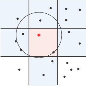
FIGURE 12-10 Other grid cells to be checked to find the nearest point
It is also entirely possible that there are no points at all in the query point’s grid cell. In this case, it is necessary to check grid cells at distances farther and farther away from the query point until a point near (but possibly not nearest) the query point is found. This checking is done a layer of cells at a time, where each layer is one grid cell farther away from the query point’s cell.
The search process can stop after the distance from the query point to the nearest point found so far is smaller than the distances from the query point to the edges of the entire layer whose points have all been compared to the query point.
Does the Query Circle Fall Within a Layer?
How can the algorithm be certain that findNearest() has found the point that is closest to the query point? After all the points within a layer have been checked, and if the query circle is enclosed by that layer, then it is certain that there are no points in farther layers that could possibly be closer to the query point. In the case of Figure 12-9, you know that there is no need to consider additional layers of cells. In the cases of Figure 12-10 and Figure 12-11, however, the query circle extends beyond the bounds of the current layer of cells, so it is necessary to consider the points in the next layer out. In Figure 12-11, the cell containing the query point is empty, forcing the search to at least include the first layer. Stopping the search at the first layer, however, would miss potentially closer points in the second layer.

FIGURE 12-11 Checking additional layers to find the nearest point
The row and column number of a cell can be turned back into the coordinates of its lower-left corner by multiplying by the private __cellSize attribute. So, given the row and column of the cell containing the query point, the __cellSize, and the number of the layer that you’re searching (assuming that the center cell containing the query point is at layer zero), it is easy to compute the left, right, top, and bottom bounds of the entire layer in either Cartesian or geographic coordinates.
For example, see Figure 12-12, where the row, col of the center query cell is at 1, 2; the current layer is 2; and the cell size is 50 units in Cartesian coordinates. Because you’re at layer 2, the entire square layer encompasses five rows and five columns of cells, each of which is 50 × 50 in Cartesian coordinates. Then the row of the bottom of the layer is 1 – 2 or –1, the row of the top layer is 1 + 2 or 3, and in terms of Cartesian coordinates

FIGURE 12-12 Determining the boundary coordinates of a layer
bottom edge: y = (–1 * 50) = –50 top edge: y = ((3 + 1) * 50) = 200
Likewise, the left and right coordinates of the current layer can be calculated from the column number of the query cell.
The __getLayerBounds() method in Listing 12-18 takes a row, column tuple specifying the cell, and a layer number as parameters, and does this computation, returning a Bounds object containing the Cartesian or geographic coordinates of the left, right, top, and bottom edges of the current layer of cells.
LISTING 12-18 Computing the Bounds of a Layer
class Grid(object):
…
    # return Bounds of the layer with cell at its center
    def __getLayerBounds(self, cell, layer):
        left = (cell[1]-layer) * self.__cellSize
        right = left + (self.__cellSize * (layer * 2 + 1))

        bottom = (cell[0]-layer) * self.__cellSize
        top = bottom + (self.__cellSize * (layer * 2 + 1))

        return Bounds(left, right, top, bottom)
It’s now a simple matter to compute whether a query circle is entirely contained within the bounds of the rectangle centered at the query point and that extends out the specified number of layers, as shown in Listing 12-19. First, you compute the location of the layer’s outer boundaries, and then you use the Bounds.within() method (refer to Listing 12-7) to determine whether the query circle’s bounding box falls within the bounds of the current layer.
LISTING 12-19 Determining Whether a Query Circle Lies Within a Layer
class Grid(object):
…
    # Returns true if the query circle falls within the specified
    # layer surrounding the search coordinates.
    # a,b are the coordinates of the query circle center
    # cbounds is the current Bounds of the query circle
    def __withinLayer(self, cBounds, a, b, layer):
        # get the bounds of the layer
        cell = self.__getCell(a, b)     # row,col of cell
        layerBounds = self.__getLayerBounds(cell, layer)

        # check if the circle's bounds are within the layer
        return cBounds.within(layerBounds)
Does the Query Circle Intersect a Grid Cell?
The computation of distances between the query point and each point in a grid cell can be computationally expensive, especially for the computation of the haversine distance, which involves multiple trigonometric function calls. But you need to consider only the points contained in those cells that intersect with the query circle, and you can ignore the cells that don’t intersect with the query circle.
Figure 12-13 illustrates five query circle sample scenarios in which might occur when determining whether any part of a query circle falls within the center grid cell. By creating a bounding box surrounding the query circles, you can then easily determine whether a query circle might intersect with the center grid cell. Of course, approximating query circles with their bounding boxes has limitations. The approximation may sometimes falsely decide that a query circle intersects a grid cell, when in reality it is the corner of the bounding box that intersects with the grid cell, but not the circle itself. We have chosen to use bounding boxes of the query circle, even at the expense of occasional additional visits to a cell, to simplify the intersection computations for highly distorted query circles that are far from the equator.
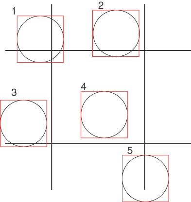
FIGURE 12-13 Determining the intersection between a query circle and a cell
If the circle’s bounding box and cell don’t intersect, as is the case for query circles 3 and 5 in Figure 12-13, then you can move on to the next cell. The intersects() method of the Bounds class in Listing 12-6 performs this intersection test (with the bounding box approximation to the query circle).
Generating the Sequence of Neighboring Cells to Visit
The search for the point closest to the query point starts at the cell containing the query point and then works outward, considering the points in cells at successive layers of distance from the query point’s cell. Figure 12-14 shows the query point in red and then the neighboring cells labeled with the row and column offset from the query cell. The layer number can be easily derived from the row, column offset by taking the maximum of the absolute values of the two offsets.

FIGURE 12-14 Offsets from the query center to each layer
The Grid class contains a static method called offsets(), written as a generator, and shown in Listing 12-20. The method yields tuples, one at a time, where each tuple is the row, column offset of the next grid cell to be visited. For each layer, offsets() first yields tuples for the cells along the sides of the layer, followed by the tuples for the corners of the layer. The corners are yielded last for each layer because the corner cells contain points that are potentially the farthest from the query point.
LISTING 12-20 A Generator to Produce Grid Offsets in Layer Order
class Grid(object):
    # Generator to yield grid offsets in concentric
    # layers, starting at the center 0,0
    @staticmethod
    def offsets():
        yield 0,0

        layer = 1
        while True:
            for num in range(-layer+1, layer):
                yield    num,  layer # yield offsets for the
                yield    num, -layer # cells along each side
                yield -layer, num
                yield  layer, num

            yield -layer,  layer # yield offsets for the
            yield  layer,  layer # corners of the layer
            yield  layer, -layer
            yield -layer, -layer

            layer += 1  # move on to the next layer
This method could hypothetically run forever, yielding an infinite sequence of successively farther layers of grid cell offsets. As you soon see, however, findNearest()stops consuming offsets from the generator after the query circle fits within a layer. As a practical matter, if there are sufficient points per grid cell, it is rare that more than one layer of neighboring cells needs to be visited.
Pulling It All Together: Implementing Grid's findNearest()
With these preliminaries out of the way, you can finally implement findNearest(). This method is a bit longer than usual, so the code comments in Listing 12-21 are annotated with lettered labels, which we expand on in the coming paragraphs.
A: If nothing has been inserted yet into the grid, there’s no need to proceed further, so just return None. This is the only scenario in which None is returned. Note that the Grid object does not keep track of the number of items it stores. The length of the Python dictionary (__cells) is the number of keys with values, so when there are no keys, no lists of points have been inserted.
B: The algorithm keeps track of the closest point seen so far, and the distance to that point. Initially, the closest point answer is None, and the distance to the closest point is math.inf. Because inf is the largest possible number, any subsequent point’s distance will necessarily be closer.
C & D: The __getCell() method converts the query point’s coordinates into the row, column of the query point’s cell. That cell is considered to be layer zero.
E: Loop over each of the grid cell offsets returned by the offsets generator. The first offset is (0,0) so that causes the search process to start at the cell containing the query point.
F: At some point, the next offset in the sequence will be one layer farther out. To determine when the layer number changes, we calculate the layer of this next offset. As seen in Figure 12-14, the layer number is the larger of the absolute values of the row and column offset values.
G: If the next offset lies in a new layer of cells, this is the opportunity to check whether it is necessary at all to loop over the cells in the new layer. So, if an answer point has been found, and if the query circle fits entirely within the previous layer (curLayer), then there is no point in proceeding with the next layer. The method breaks out of the offset loop to return the best answer point so far. Otherwise, it records the next offset’s layer as the current layer.
H: Having arrived at a new offset cell to search, findNearest() retrieves the list of points stored there. The cell’s row and column are obtained by adding the offsets to the query point cell’s row, column.
I: Now we’re ready to decide whether to do the work to compare all the points in the new cell to the query point. Comparisons are only needed if there are some points in the cell, and if the query circle intersects the cell. Initially, when an answer hasn’t yet been found, perhaps because all the grid cells so far have been empty, the distance is still infinity, so the query circle will intersect every cell. But if the query circle doesn’t intersect the cell, then none of the points could possibly be closer to the closest point encountered so far.
J: Looping through each of the points in the current cell, compute the distance from the point to the query point. If the distance is exactly zero, this means that search has found an exact match to the query point and can return the point and its data. Otherwise, if the distance to the query point is less than the smallest distance found so far, remember the new candidate point and its distance. Because the distance to the nearest point has now decreased, the method invokes CircleBounds.adjust() to recompute the bounding box for the smaller query circle.
K: There’s only one way to make it to this line of code. Namely, that the break statement was executed during step G because an answer was found and because the query circle was entirely contained within the previous layer of searched cells. The findNearest() method returns the coordinates of the point, the data stored with that point, and the distance from the query point to the answer (that is, nearest) point.
This process may seem complex. Yet, as we show at the end of the chapter, in certain situations this Grid.findNearest() can perform significantly better than the theoretically superior QuadTree code.
LISTING 12-21 The findNearest() Method for Grid
class Grid(object):
…
    def findNearest(self, a, b): # find the closest point to (a,b)
        if len(self.__cells) == 0:  # A: Nothing in grid yet
            return None

        answer = None  # B: remember the closest point so far

        # The current search circle and its bounds so far
        distance = inf
        cBounds = CircleBounds(a, b, distance, self.__distance)

        cell = self.__getCell(a, b) # C: cell containing a,b
        curLayer = 0                # D: the layer we're up to

        # E: for each offset
        for off in Grid.offsets():
            #F: what layer is this new offset?
            layer = max(abs(off[0]), abs(off[1]))

            # G: if we're about to consider a new layer,
            # but the search circle falls entirely within
            # the prior layer, then there's no need to continue.
            if layer != curLayer and answer and
               self.__withinLayer(cBounds, a, b, curLayer):
                break
            curLayer = layer # remember what layer we're up to

            # H: get the points stored in the cell at that offset
            offsetCell = cell[0]+off[0], cell[1]+off[1]
            points = self.__cells.get(offsetCell, None)

            # I: if there are points in the cell, and
            # the search circle intersects the cell...
            if points and
               cBounds.intersects(self.__getCellBounds(offsetCell)):

                for p in points: # J: for each point in the grid cell
                    # compute distance to that point from query point
                    newDist = self.__distance(a, b, p[0], p[1])

                    if newDist == 0: # exact match?
                        return p[0], p[1], p[2], 0

                    if newDist < distance:  # new point closer?
                        distance = newDist  # remember the distance
                        answer = p          # and the point, and
                        cBounds.adjust(distance) # adjust bounds

        # K: returns a, b, data, distance to query point
        return answer[0], answer[1], answer[2], distance
Quadtrees
In the previous sections, you saw that a grid is an excellent data structure for searching points when the data is somewhat uniformly spread out because each grid cell contains a relatively equal number of points for searching. But what happens if the data is not so uniformly spread out? Figure 12-15 shows about 30,000 points. Each of the clusters has about one-third of the points. This kind of clustered data is typical in the real world. For example, locations of restaurants, coffee shops, and other businesses tend to be clustered near each other.

FIGURE 12-15 Thirty thousand highly clustered points
Overlaying a grid on top of this data, as shown in Figure 12-16, makes it clear that for clustered data a grid doesn’t offer much benefit. Searching for a point inside the red-outlined grid cell near the bottom would involve processing nearly all the points in that cluster.
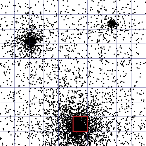
FIGURE 12-16 Uniform grid dividing the 30,000 points
Many of the grid cells are empty or contain just a few points, while most of the points are concentrated in a small number of the grid cells. As one solution, you could decrease the size of every one of the grid cells. So instead of a grid of 10 × 10 cells overall, you’d use a grid of 100 × 100 cells for a total of 10,000 grid cells to store the 30,000 points. Figure 12-17 zooms in to look at just one of the 10 × 10 cells, the red-outlined one, which contains several thousand points.
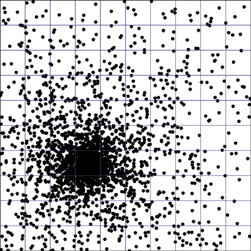
FIGURE 12-17 A finer grid on just one of the point clusters
At this scale, because you are now using a 100 × 100 grid, what used to be a single grid cell is now itself composed of 10 × 10 of the smaller cells. And again, most of the points are heavily concentrated within a small fraction of the cells, while most of the cells contain a relatively small number of points.
This is the dilemma with using fixed grids where the cell size is uniform across all the data. Real-life data tends to be very unevenly distributed. At whatever scale of magnification that you use to examine the data, clusters tend to be apparent. The implication is that no matter how fine the grid is made, some areas of space would benefit from a finer grid.
Quadtrees, also written as quad trees, were invented in the early 1970’s by Raphael Finkel and Jon Bentley, and provide an elegant solution to this problem. A quadtree is a tree data structure that recursively divides up space into four quadrants. Parts of the quadtree that contain more points are further divided into finer-sized quadrants. Parts of the quadtree that contain fewer points divide space into larger quadrants. Adaptively subdividing space based on the density of spatial data makes it possible to insert or search for points in O(log4 N) time, or as you saw in Chapter 2, “Arrays,” more simply just O(log N) time.
This tree-like structure probably looks familiar. The different kinds of trees you studied in Chapters 8, 9, and 10 were all organized by dividing the items by their keys. Quadtrees do something similar but with two numeric values. A binary search tree with a single numeric key inserts items with lower-valued keys in the left subtree and higher-valued keys in the right subtree. With spatial data, you can do something similar, but this time with quadrants.
In the following pages, we look in more detail at a quadtree implementation using the same methods that were implemented for the PointList and Grid classes: a constructor, insert(), findExact(), findNearest(), delete(), and traverse().
Creating an Instance of the QuadTree Class
Client code creates an instance of the QuadTree class by invoking the constructor to create an object that contains Cartesian points:
q = QuadTree('cartesian')or that contains geographic points:
q = QuadTree('geographic')If the constructor is passed any string other than 'cartesian' or 'geographic', an exception is raised.
Listing 12-22 shows the code for the QuadTree constructor. It has just two private attributes: a reference to the distance function appropriate to either Cartesian or geographic coordinates, and an initially empty reference to the root node of the tree.
LISTING 12-22 The QuadTree Constructor
class QuadTree(object):

    def __init__(self, kind): # must specify type of coordinate
        if kind == 'cartesian':
            self.__distance = euclideanDistance
        elif kind == 'geographic':
            self.__distance = haversineDistance
        else:
            raise Exception("Invalid kind of coordinate")

        self.__root = None
Inserting Points: A Conceptual Overview
Let’s look at the first few inserts of points into an initially empty quadtree, with each new point finding its place in the quadtree through a recursive descent. Each node in a quadtree potentially has four children, corresponding to the northeast, southeast, southwest, and northwest quadrants of space that surround that point. The first point to be inserted into the quadtree becomes the root of the tree (labeled point A in Figure 12-18), and the four children of that node all refer to None.

FIGURE 12-18 Inserting the root point in a QuadTree
Next, as shown in Figure 12-19, another point, labeled B, is inserted. Starting at the root, the coordinates of the new point are compared against the coordinates of the root node A. Point B lies to the southwest of point A, so you recursively descend to the corresponding child of point A. Because the southwest child currently refers to None, a new node is created to contain B, and upon return from the recursion, the southwest child of A is made to refer to B.

FIGURE 12-19 Inserting point B
The next point, labeled C, is inserted, as shown in Figure 12-20. Again, starting from the root node, C is compared to the coordinates of point A. Point C lies to the southeast of A, so the recursion proceeds to the southeast child, and because it is found to be None, a new node is created containing the coordinates of point C, which is then returned from the recursion and assigned to the southeast child of A.

FIGURE 12-20 Inserting point C
Finally, as shown in Figure 12-21, a point, labeled D, is recursively inserted into the tree, starting at the root point A. Because D lies in the southwest quadrant of A, the recursion then proceeds to point B, which is the southwest child of point A. The coordinates of point D are northwest of the coordinates of point B, so the recursion then proceeds to the northwest child of B. Having reached None, a new node is created to hold point D, which is then returned from the recursion. Upon returning to point B, the northwest child of B is set to refer to the just-returned reference to the newly created point D.

FIGURE 12-21 Inserting point D
Avoiding Ambiguity
When recursively descending a quadtree either for insertion or searching, it is important to make a consistent decision at each node regarding which child to descend into. If a point is properly within a quadrant, then there is no ambiguity. But which quadrant should be chosen if an inserted or searched point lies directly above or below, or directly to the right or left of a node? For example, in Figure 12-22, to which quadrant of A does point B belong?
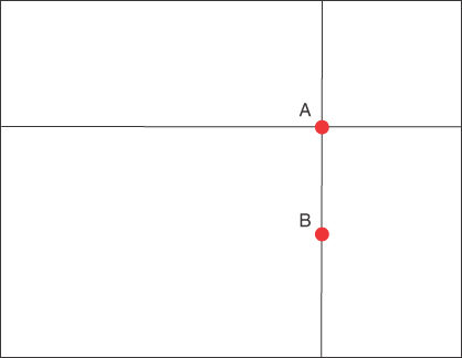
FIGURE 12-22 Quadrant ambiguity
Whatever solution we choose, we must make certain to apply it consistently. Our solution to this problem is to have the points on each of the four axis boundary lines belong to the quadrant that is clockwise of the axis line. So, in Figure 12-22, B would belong to the southwest quadrant of A.
More generally, as shown in Figure 12-23, the points that are exactly above the node’s point all belong to the node’s northeast quadrant. The points that are exactly to the right of the quadtree node belong to the node’s southeast quadrant, and so on.

FIGURE 12-23 Assignment of axis boundary lines to quadrants
The QuadTree Visualization Tool
To see how quadtrees operate, you can run the QuadTree Visualization tool. The tool can be used to manage Cartesian point data in a rectangular region, as shown in Figure 12-24. The points are shown as dots with a label above them that represents the “data” associated with a point.
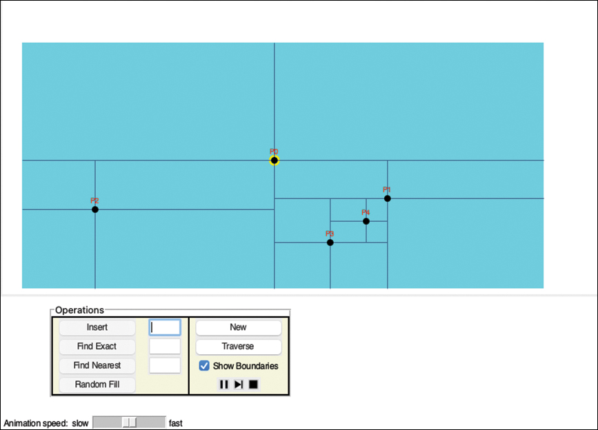
FIGURE 12-24 The QuadTree Visualization tool
You can insert new points in two ways: by double-clicking with a pointer (mouse) button in the light blue region, or by entering an X coordinate, Y coordinate, and data label in the three text boxes and selecting the Insert button.
The first point inserted becomes the root of the quadtree and is highlighted in yellow. When you insert points by double-clicking, the tool automatically chooses the data label in the form P0, P1, P2, and so on, based on the current number of points in the quadtree. When you type the coordinates, they are relative to the origin, point (0, 0), at the lower left of the region. You can provide any short string for the data (as long as the points have unique names).
The quadrants around each point are visible when the boundaries between them are displayed. If you uncheck the Show Boundaries checkbox, you will see only the points, making their tree relationship invisible. Finding the parent of a node is somewhat tricky. You must look at the boundaries, follow them to their endpoint, and then follow the crossing boundary to see whether it intersects a labeled node. For example, in Figure 12-24, P3’s parent is P1, and two of P3’s boundary lines end on the boundary lines of P1. The parent of P4 is harder to see because both P1 and P3 look equally likely based on the closest boundary lines. You must look at the extent of the boundaries of the two potential parents to resolve the ambiguity. P0, the root, has boundary lines that extend all the way to the blue region boundaries, and those have no boundary lines leading to another node.
Try inserting a few points by typing the coordinates for the points. By giving exact coordinates, you can insert new points on a quadrant boundary. Based on the rule in Figure 12-23, you should be able to predict the quadrant of the new point. The (single) boundary line drawn for it spans that quadrant. The other boundary line overlaps the boundary line where the point lies, so it is not visible. You can also click an existing point to copy its coordinates and label to the text input boxes. From there, you can edit the values to insert a new point that lands exactly on one of its quadrant boundaries. Clicking the blue region where there are no points simply enters the two coordinates into the text boxes.
Implementing Quadtrees: The Node Class
Just as with other types of trees, you can define a class to correspond to the nodes within a quadtree, as shown in Listing 12-23. The Node class and its attributes don’t have to be made private because the QuadTree class will never directly return an object of the Node type, and therefore, encapsulation will not be violated.
LISTING 12-23 The Node Class
class Node(object):
    # a,b corresponds to either x,y or long,lat
    def __init__(self, a, b, data):
        self.a = a  # coordinates of the point
        self.b = b
        self.data = data # data associated with point

        # Four children of the Node
        self.NE = self.SE = self.SW = self.NW = None
Having seen the constructors you may wonder, where in the Node or QuadTree classes are the boundary lines for each quadrant stored? The answer is that the boundary lines are not explicitly stored anywhere! Rather, you can think about the a, b coordinates of each Node as establishing the boundaries that subdivide all of the space surrounding the point into four quadrants. For example, the southeast quadrant of a Node has its top boundary specified by the b coordinate, and its left boundary specified by its a coordinate. But what about the bottom and right boundaries? Those boundaries are not explicitly stored in the Node objects; rather, they are implicit. That is partially the reason why it is difficult to see the parent-child relationships from the boundaries shown in the visualization tool—the boundaries of a child extend to its parent’s boundaries.
As you will see shortly, the implementation of findNearest() search recursively descends the quadtree, progressively refining the boundaries of the space of the quadrant being visited. For example, the boundaries of the root Node at (a, b) are, respectively:
left: -math.inf, right: math.inf, top: math.inf, bottom: -math.inf
In other words, the root node’s space encompasses all points in the plane. Suppose you descend to the southeast corner of the root node, P0, which would be node P1 in Figure 12-24. Then you can refine the boundaries for the southeast quadrant of P0 at (a, b) to be
left: a, right: math.inf, top: b, bottom: -math.inf
In other words, the southeast quadrant of the root is thought of as being unbound to the right and downward. As you descend farther into the tree, the left, right, top, and bottom boundaries get updated to reflect the subset of the plane that is associated with a child Node. In many parts of the implementation, however, these boundaries don’t need to be explicitly stored. For example, they are not needed for insertion. We discuss the explicit boundaries in more detail when we discuss findNearest().
The insert Method
QuadTree clients insert point data using an insert() method with the same signature as those in PointList and Grid. Listing 12-24 shows the Python code for insert() and its companion method, __insert().
The insert() method is a wrapper method whose sole function is to invoke the recursive __insert() method, passing to it the root of the quadtree. Whatever __insert() returns is then assigned back to the __root attribute. This unusual pattern is worthy of some discussion, as you may recall from when it was used in Chapter 10, “AVL and Red-Black Trees,” for AVLTree objects.
Why should insert() need to reassign a value for __root upon every invocation? Consider the case when the quadtree does not yet contain any points, and therefore __root refers to None. When insert() invokes __insert(), a new Node object is created and then returned immediately to insert(), which then assigns it to __root. That makes sense! But what about subsequent invocations of insert()? Would its recursive call to __insert() ever return a reference to a different Node? No, it would not. But that is OK, because the assignment to self.__root just ends up assigning the same Node to it that is already there! As you look more carefully at __insert(), you’ll see that you can ask the same question regarding the returns from all the layers of recursion.
LISTING 12-24 The insert() Method of QuadTree
class QuadTree(object):
…
    def insert(self, a, b, data): # Wrapper. Always succeeds.
        self.__root = self.__insert(self.__root, a, b, data)

    # Recursive private method that does the inserting
    def __insert(self, n, a, b, data):

        # return a new Node if we've reached None
        if not n: return Node(a, b, data)

        # if the point to be inserted is identical to current node,
        # overwrite the data, and don't recurse any further
        if n.a == a and n.b == b:
            n.data = data
            return n

        # recurse down into the appropriate quadrant
        if   a >= n.a and b >  n.b: n.NE=self.__insert(n.NE,a,b,data)
        elif a >  n.a and b <= n.b: n.SE=self.__insert(n.SE,a,b,data)
        elif a <= n.a and b <  n.b: n.SW=self.__insert(n.SW,a,b,data)
        else:                       n.NW=self.__insert(n.NW,a,b,data)
           # a <  n.a and b >= n.b

        return n
Moving on to __insert(), the method takes as parameters a reference to the current Node n in the QuadTree, along with the a, b coordinates and the associated data for the point to be inserted. In the first step, if __insert() reaches an empty child node (None), then it creates a new Node and returns it. The caller might have been the insert() wrapper, in which case the new Node will be assigned to self.__root. The caller could also have been one of the recursive invocations of __insert() later in the method. When those invocations return, the returned newly created Node gets assigned into the quadrant attribute that until now referred to None.
If n refers to anything other than None, then the next check is for the possibility that the newly inserted point a, b and the current node n both refer to the exact same coordinates. We made a design decision that QuadTree objects will not support multiple points with the duplicate coordinates. So, if there is an exact match, then the newly inserted data will overwrite the existing data stored for those coordinates, and then __insert() can return a reference to the current node n. We leave it as an exercise to explore how to insert points with duplicate coordinates.
Finally, the real work of the recursion happens. At this point of the __insert() method, a, b can’t possibly be an exact match to n’s coordinates. The a, b coordinates of the inserted point are compared to the coordinates of the current node n to decide which quadrant should receive the new point. Let’s take a careful look at the first of these four similar recursion decisions:
if a >= n.a and b > n.b: n.NE = self.__insert(n.NE, a, b, data)
Notice that points will end up in the northeast quadrant if the a coordinate is greater than or equal to the current Node’s a coordinate and if the b coordinate is greater than the current Node’s b coordinate. But that is exactly the decision that we illustrated in Figure 12-23: ambiguous points are placed in the quadrant clockwise away from the boundary where they lie. The decisions for recursion into the other three quadrants are likewise consistent with the figure.
Also notice the peculiar form of the recursive invocation. It recursively passes n.NE into __insert(), and then whatever the invocation of __insert returns gets assigned right back into n.NE! This is just a variation of the first invocation of __insert() by the insert() wrapper method. Here, when __insert() is recursively invoked, n.NE might be None, or it might already refer to a child Node. If n.NE is None, then immediately upon the recursive invocation, __insert() will create and return a new Node containing the inserted a, b data point. The caller appropriately assigns the new node to n.NE. If n.NE is not None and already refers to a child Node, then __insert() will necessarily end up returning that very Node, which then gets harmlessly assigned back to n.NE.
Appropriately, the last line of __insert() causes a reference to the current Node n to be returned to the calling method.
In summary, there are three possible returns from the recursion:
A reference to a brand-new
Nodeis returned if the recursion reached an empty node represented asNone.If a duplicate point was inserted, after overwriting the current node’s data with the newly inserted data, a reference to the current
Nodeis returned.A reference to the current
Nodenis returned if the insertion recursively occurred somewhere below the currentNode.
In all three cases, what is returned to the calling method is a reference to the Node that belongs at that point in the QuadTree. Most of the time, the returned value references a Node that has already been created and that is already referred to by one of the child attributes of the parent Node.
Another way to think about this is to imagine the process involved in inserting a point with new coordinates 10 levels down into the QuadTree. You recurse down 10 levels into the appropriate quadrants and reach a child attribute containing None. At that point, you create a new Node, and it is returned to be assigned to the parent’s appropriate child attribute. As the recursion then “unwinds” all the way back to the root, each intermediate Node is just returned to the calling method, which then harmlessly assigns the Node back to the child attribute that already contains that reference.
Try stepping through the insertion of a point using the visualization tool. It shows how each recursive call to __insert() checks the relationship of the new point’s coordinates with those of a node in the tree and then either descends to a child node, creates a new node, or updates the data of an existing one. As the recursion unwinds, the nodes visited along the path to the new or updated node are returned to their parent.
Efficiency of Insertion
If the quadtree is relatively well balanced, then inserts into the quadtree should take O(log N) time, so inserting N points would take O(N × log N) time. Just as with binary search trees, degenerate sequences of inserts can cause the tree to be very unbalanced. For example, if points were inserted in order along a southwest diagonal line, the result would be the worst possible case, with each insertion taking O(N) time, resulting in O(N2) time to insert N points. You see shortly that such an unbalanced quadtree degrades the performance of searching, too.
Dynamic rebalancing of a QuadTree in a manner like an AVL tree is possible but very complex. If an application has all, or even most, of the points in advance that need to be stored in a QuadTree, then a bulk insert method can arrange for the tree to be better balanced. We leave this method for you to complete as an exercise at the end of the chapter.
Finding an Exact Match
The client uses the findExact() method to search for the point contained in the QuadTree object that exactly matches the specified x, y or longitude, latitude coordinates. If an exact match is found, the method returns a reference to the data stored for the matching point. The client uses findExact() in the same fashion as with the PointList and Grid classes.
Finding an exact match is a simple process, as shown in Listing 12-25. If the QuadTree contains an exact match, then a recursive descent that mirrors the descent used by insert() is guaranteed to find the matching point.
Like the insert() method, you can use a wrapper method called findExact() to start the recursion by passing the root node into the recursive __find() method and simply returning its result. The first base case occurs if the recursion has reached a None (empty leaf) value. If this happens, it is certain that there’s no exact match for a, b and None should be returned to indicate that no point was found, and therefore no data returned.
Another base case occurs if the search has reached a node that exactly matches a, b. In this case, the associated data is returned and makes its way back to the wrapper method as the recursion unwinds.
Otherwise, if an exact match to a, b is anywhere in the quadtree, it must be in the quadrant that encloses a, b. So, just as was done for insertion, you recursively descend into the appropriate quadrant, and you return whatever is returned by the recursive call. If the recursion reaches None, then it is certain that there’s no node that matches the specified coordinate.
LISTING 12-25 The findExact() Method of QuadTree
class QuadTree(object):
…
    # Wrapper method - returns the data object associated with a,b
    def findExact(self, a, b): return self.__find(self.__root, a, b)

    def __find(self, n, a, b):
        if not n: return None  # Couldn't find the exact point

        # Did we find the exact point? Return the data
        if n.a == a and n.b == b: return n.data

        # Recurse down into the appropriate quadrant.
        # If a,b is anywhere, it MUST be in that quadrant.
        if   a >= n.a and b >  n.b: return self.__find(n.NE, a, b)
        elif a >  n.a and b <= n.b: return self.__find(n.SE, a, b)
        elif a <= n.a and b <  n.b: return self.__find(n.SW, a, b)
        else:                       return self.__find(n.NW, a, b)
           # a <  n.a and b >= n.b
Try a few exact searches with the visualization tool to watch this process. Create a few points in the quadtree and then click a region with no points. Doing so fills in the coordinates of the clicked point in the arguments area and enables the Find Exact operation. Select the Find Exact button. It draws a cross at the clicked point and makes the recursive calls to __find() as it checks the relationship of a, b to each node. You can also click an existing point to verify that findExact() follows the nodes in the tree to that point.
Efficiency of Exact Search
If the quadtree is relatively well balanced, then finding an exact match for a point in a quadtree should take O(log N) time, though in the worst case with a completely unbalanced tree, findExact() could be as bad as O(N). This degenerate performance makes it no better than the operation in a simple PointList, although it is very unlikely to occur with data that is inserted in a random order with respect to spatial position.
Traversing the Points
Just as we did with PointList and Grid, QuadTree’s traverse() implementation should be done as a generator. The natural way to traverse a QuadTree is to do a pre-order recursion, starting at the root, and then recursively visiting and yielding each of the nodes in the tree, followed by each node’s children. Mixing recursion with generators poses a challenge because it is difficult to write efficient recursive generators in Python.
As we discussed in Chapter 6, “Recursion,” every recursive function can be transformed into a nonrecursive version by using a stack. We showed this transformation in Chapter 8, "Binary Trees.” Listing 12-26 shows a similar nonrecursive implementation of traverse(), where we use a Python list to implement the two required stack operations of push (using list’s append() and pop() methods). Alternately, it would be straightforward to use the Stack class from Chapter 4, “Stacks and Queues,” if you know the number of points in the quadtree, or the LinkStack class from Chapter 5, “Linked Lists,” if you don’t.
LISTING 12-26 The traverse() Method of QuadTree
class QuadTree(object):
…
   def traverse(self):
        s = [ ]   # initialize stack with root
        if self.__root: s.append(self.__root)

        while len(s) > 0: # stack's not empty?

            # process Node at top of stack
            n = s.pop()
            yield n.a, n.b, n.data

            # push each child onto stack
            if n.NE: s.append(n.NE)
            if n.SE: s.append(n.SE)
            if n.SW: s.append(n.SW)
            if n.NW: s.append(n.NW)
The method starts by initializing the stack to contain just the root Node. Then, as long as the stack isn’t empty, you pop the top Node from the stack and yield its coordinates and data. Finally, any children of the Node are pushed onto the stack.
This implementation seems more complex than the corresponding traverse() methods in the PointList and Grid classes. What is its Big O complexity?
With a bit of analysis, we can determine that the quadtree’s traverse is also O(N). We determine this by focusing on the pushes and pops of points to and from the stack. Examining the code, we can see that each Node is pushed just once onto the stack, and that each Node is ultimately popped (and yielded) just once from the stack, corresponding to each pass through the while loop. Thus, for a QuadTree containing N nodes, the traversal can be accomplished with N passes through the while loop, and a total of N pushes and N pops. These roughly 3N operations correspond to O(N) complexity for the traverse() method.
Deleting a Point
To locate a point to delete, you should use the same approach as used in findExact(). If the matching point is identified, it needs to be deleted. If not, an exception should be raised.
Removing a leaf node from a quadtree should be relatively simple. What should the method do, however, if the matching node is an interior node of the quadtree? Because a Node can’t be easily removed from the quadtree without rebuilding the structure of its children, one reasonable approach would be to leave the Node in place, and instead set its data attribute to None. Thus, any Node with a data attribute containing None would not subsequently be treated as a valid data point stored in the quadtree. If the quadtree must support None as a legitimate data value for a point, then a special sentinel value must be inserted that can be distinguished from None. The __Deleted sentinel performs this role for open addressing hash tables (as described in Chapter 11, “Hash Tables”).
Marking the data attribute as deleted means that small changes are needed to the findExact() method (in Listing 12-25) and the findNearest() method (described in the following sections) so that nodes without data are never considered as valid matching points. These data-less nodes take some extra memory but still provide useful information about where space is subdivided into quadrants.
Because delete() must first find the node like findExact(), the Big O must be at least O(log N). The rest of the work (removing a leaf node or inserting a no-data marker in the data attribute of an interior node) takes a few steps but does not depend on the number of items in the quadtree, so it adds nothing to the overall complexity. If many interior nodes are deleted, the tree does not shrink, so the N in O(log N) is the total number of inserted items, not the current number of items in the tree, for deletion, insertion, and search.
We leave it as a Programming Project for you to implement a method to delete a point specified by a pair of coordinates from the quadtree. The visualization tool does not have a delete operation, but you can erase all points with the New button and then insert new points.
Finding the Nearest Match
As usual, finding the nearest match via the findNearest() method is more complicated than findExact(). Just as with the Grid class, merely descending into the appropriate quadtree quadrant does not guarantee that you have found the nearest match to the search coordinates.
For example, in Figure 12-25, if you descend into the QuadTree to find the deepest node whose boundaries surround the red diamond query point (outlined in red), you can use that deepest point as a good candidate for the nearest match. However, if you draw a circle with the query point at its center and its radius matching the distance to the candidate, it becomes clear that any quadrant that is overlapped by the circle might conceivably contain a closer node and must therefore be considered. Those quadrants that you must visit are shaded in light blue. The example shows that there is a point in the query circle that was not visited on the path to the candidate (because the search from the root node—the one whose quadrant boundaries span the entire figure—followed the path to the NW, then NE, and then SW quadrants based on the query point). How do you ensure that those other quadrants shaded in blue are visited during the search?
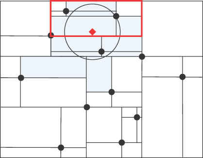
FIGURE 12-25 Additional quadrants to be visited based on query circle
Similar to how the Grid object had to intersect a query circle with the various cells, there’s a way to compare quadtree boundaries with the query circle to minimize the quadrants to explore. Let’s look at the implementation details to complete your understanding of how to find the nearest Node to a query point.
Finding a Candidate Node
Let’s start by following the logic used in findExact() to get a point somewhere in the vicinity of the query point. Listing 12-27 shows the private __nearPoint method. As you soon see, findNearest() invokes this method by passing in __root and the a, b search coordinates.
LISTING 12-27 The __nearPoint() Method
class QuadTree(object):
…
    # find a nearby (but not necessarily the nearest) point
    # to a,b by recursing as deep as possible into the tree.
    def __nearPoint(self, n, a, b):
        # Base cases:
        if not n: return None # reached None so return it

        if a == n.a and b == n.b: return n # found exact point

        # recurse down into the appropriate quadrant
        if   a >= n.a and b >  n.b: ans = self.__nearPoint(n.NE, a, b)
        elif a >  n.a and b <= n.b: ans = self.__nearPoint(n.SE, a, b)
        elif a <= n.a and b <  n.b: ans = self.__nearPoint(n.SW, a, b)
        else:                       ans = self.__nearPoint(n.NW, a, b)
           # a <  n.a and b >= n.b

        # if we found a lower Node near this point return it
        # otherwise return the current node
        return ans if ans else n
The __nearPoint() method returns the deepest Node in the tree along the path from the root toward the query point. It does so by recursively descending into the QuadTree in a fashion almost identical to __find(). Instead of returning the corresponding data if an exact match is found to a, b, __nearPoint() returns a reference to the Node that either matches a, b exactly, or is as deep as possible in the QuadTree.
Not surprisingly, the base cases are similar to __find(). If __nearPoint() reaches None, then None is returned. If it reaches a node whose coordinates exactly match a, b, then that Node (n) is returned.
Otherwise, it recursively descends into the quadrant containing the query point and stores in ans whatever is returned by the recursive invocation. There are only two possibilities after the recursive call. One possibility is that ans is None because __nearPoint() just descended into an empty child. If that happens, then it means that the current node n has no descendants in the query quadrant, and therefore it returns the current node, n. Otherwise, if ans is anything but None, it means that the recursion is returning a reference to the lowest possible Node, which is then returned to its caller.
Finding the Closest Node
After __nearPoint() has discovered a candidate for the Node nearest to a, b, the __nearest() method shown in Listing 12-28 can recursively descend the quadtree again, starting at the root, trying to find successively closer candidates. This method computes the distance from the query point to the coordinates of each Node visited. If the distance is smaller than the distance to the so-far best candidate Node, then the current node, n, becomes the new, closer candidate, cand.
LISTING 12-28 Recursively Refine Nearest Candidate
class QuadTree(object):
…
    # Returns the nearest Node and distance to query point a,b.
    def __nearest(self, n, # current Node being visit
                  a, b,    # query point
                  dist,    # distance to candidate
                  cand,    # best candidate so far
                  bounds): # Bounds of current quadrant

        # Reached a None node, or already found
        # a perfect match? Return our answer.
        if not n or dist == 0: return cand, dist

        # Is the current quad tree point closer than
        # the candidate? If so, update the candidate
        fn = self.__distance
        newDist  = fn(a, b, n.a, n.b)
        if newDist < dist:
            cand = n
            dist = newDist
        # bounding box surrounding the search circle
        cBounds = CircleBounds(a, b, dist, fn)

        # For each child node - update bounds for that quadrant
        # if the search circle's bounds intersects the child
        # quadrant's new bounds, descend to that child node.
        newB = bounds.adjusted(left = n.a, top = n.b)
        if cBounds.intersects(newB):
            cand, dist = self.__nearest(n.SE, a, b, dist, cand, newB)
            cBounds.adjust(dist) # adjust the circle's bounds

        # likewise for the other three quadrants
        newB = bounds.adjusted(left = n.a, bottom = n.b)
        if cBounds.intersects(newB):
            cand, dist = self.__nearest(n.NE, a, b, dist, cand, newB)
            cBounds.adjust(dist)

        newB = bounds.adjusted(right = n.a, top = n.b)
        if cBounds.intersects(newB):
            cand, dist = self.__nearest(n.SW, a, b, dist, cand, newB)
            cBounds.adjust(dist)

        newB = bounds.adjusted(right = n.a, bottom = n.b)
        if cBounds.intersects(newB):
            cand, dist = self.__nearest(n.NW, a, b, dist, cand, newB)
            # no need to update circle's bounds after last quadrant

        return cand, dist # best candidate seen so far
In the Grid class, you saw how the intersects() method determines whether the query circle’s bounds intersect a grid cell and, therefore, whether to consider the points within the cell. QuadTree’s __nearest() method also uses the same intersects() method to determine whether the query circle’s bounds intersect any of the quadrants below the current node and, therefore, whether to continue the recursion into that quadrant. To make that determination, __nearest() must manage Bounds objects for both the query circle and the quadrants associated with node n. The bounds parameter passed from the parent holds node n’s boundaries, and the cBounds variable is set to be the query circle’s bounds using the new nearest distance to n. As the algorithm descends into each node’s quadrants, these bounds will be updated, as described shortly.
Each return from the four possible recursive calls to __nearest()returns either the same candidate and distance that were just passed to the __nearest() recursion or a closer candidate and distance that the recursion discovered. Because it is possible that a recursive call may have decreased the distance to the nearest candidate, __nearest also invokes CircleBound’s adjust() to adjust the bounding box around the current query circle. Having possibly checked all four quadrants, __nearest() then returns the best candidate and distance that was found.
There is some subtlety in how __nearest() uses Bounds.intersects(). As previously discussed, Node objects do not explicitly store the specific boundaries of the rectangle of space that they cover. Rather, each node stores just two of the boundaries, defined as appropriate, by the a coordinate (for either the left or right boundary) and by the b coordinate for either the top or bottom boundary.
How do you determine all four boundaries that define the rectangle surrounding each node? Consider Figure 12-26, which shows a QuadTree containing just three nodes: a root, G, drawn in green; its northeast child, P, drawn in purple; and P’s southeast child C, drawn in (cobalt) blue. The nodes form a grandparent (G), parent (P), and child (C) relationship. The figure also shows the Cartesian coordinates for each of the three points.
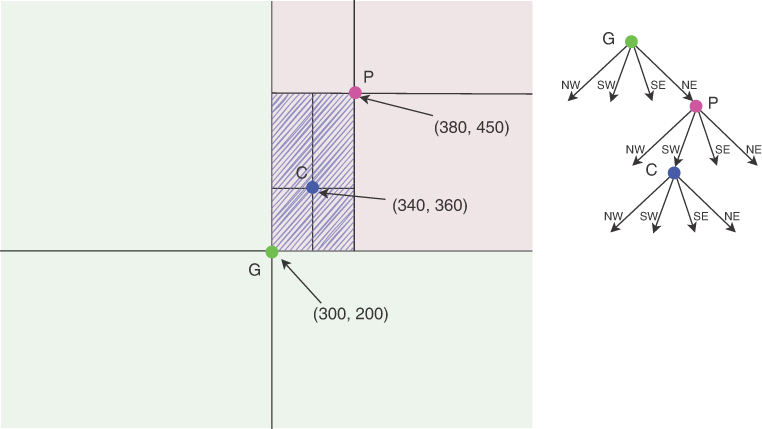
FIGURE 12-26 The intersection of ancestor quadrants forms a child's quadrant
What are the left, right, top, and bottom bounds of G’s region of space? Because G is the root, its region of the plane is unbounded. In other words, its bounds are
left: -math.inf, right: math.inf, top: math.inf, bottom: -math.inf
When the search recursively descends to G’s northeast child, node P, what are P’s bounds? P’s top and right bounds are still at infinity. However, P’s left boundary is at G’s a coordinate, 300, and P’s bottom boundary is at G’s b coordinate, 200. In other words, the bounds of P’s region are
left: 300, right: math.inf, top: math.inf, bottom: 200
Taking one more step, what happens when the search recursively descends to P’s southwest child, C. What are C’s bounds (as shown in cross-hatched blue)? C’s top boundary is defined by P’s b coordinate 450, and C’s right boundary is defined by P’s a coordinate, 380. C’s other boundaries are inherited from P. In other words, the bounds of C’s region are
left: 300, right: 380, top: 450, bottom: 200
Each time you descend to a deeper node in the quadtree, the bounds for that child node are refined by replacing the appropriate two of the four bounds with the coordinates of the current node. In other words, the bounds of a node in the quadtree are formed by the intersection of the quadrant bounding boxes in the path from the root to that node.
Based on this understanding, take another look at the code for __nearest() in Listing 12-28. For each of the four child quadrants, the method uses Bounds.adjusted() to create a new Bounds object, newB, appropriately updated to reflect the bounds of that child based on the bounds of its parent. That newB object determines whether the search circle’s bounds intersect the child’s quadrant’s bounds.
Pulling It All Together: Implementing QuadTree's findNearest()
As shown in Listing 12-29, the public findNearest() method proceeds as follows. First, using the __nearPoint() method, it finds a candidate node, ans, by recursively descending from the root as far as possible into the quadtree. Then it computes the distance from the query point to the candidate node. This is the best answer so far, even though it’s a rough approximation (unless the query point matches one of the points exactly). The candidate node and the distance from it to the query point define a query circle centered at the query point, with a radius equal to the distance to the initial candidate node.
LISTING 12-29 The findNearest() Method of QuadTree
class QuadTree(object):
…
    # returns a,b,data,distance of point nearest to query a,b.
    def findNearest(self, a, b):
        if not self.__root: return None # No points yet!

        # Descend the tree and find the leaf node nearby
        # to this query point. This quickly sets an upper
        # bound on the nearest possible point
        ans  = self.__nearPoint(self.__root, a, b)
        dist = self.__distance(a, b, ans.a, ans.b)

        # Now we will descend the tree once more, refining
        # the candidate by progressively shrinking the radius.
        # The bounds of the root node are infinite.
        bounds =  Bounds()
        ans,dist = self.__nearest(self.__root, a,b, dist, ans, bounds)

        return ans.a, ans.b, ans.data, dist
Next, the findNearest() method constructs a Bounds object for the infinite extent of the root node. The root node, the query point, the current best candidate answer, and the infinite bounds are passed to the __nearest() method to begin the recursive search, which descends into any quadrant that is overlapped by the current query circle. Each time it encounters a Node that is closer to the query point than the current candidate, the candidate is replaced, and the radius of the query circle gets smaller. The result of the recursive call on the root node provides all the return values for the complete search.
The QuadTree Visualization tool makes it easier to see how the nodes are visited, how the distances change the query circle bounds, and how the bounds overlap. We show an example using the tool of a find nearest search starting, in Figure 12-27. It begins by descending the 7-node quadtree to find the leaf node closest to the a, b query point. Starting at the root, P0, it goes to the southeast quadrant to visit P2. The query point lies in P2’s northwest quadrant, so __nearPoint() descends to P5. P5 is a leaf node, so returns it as the answer, ans.
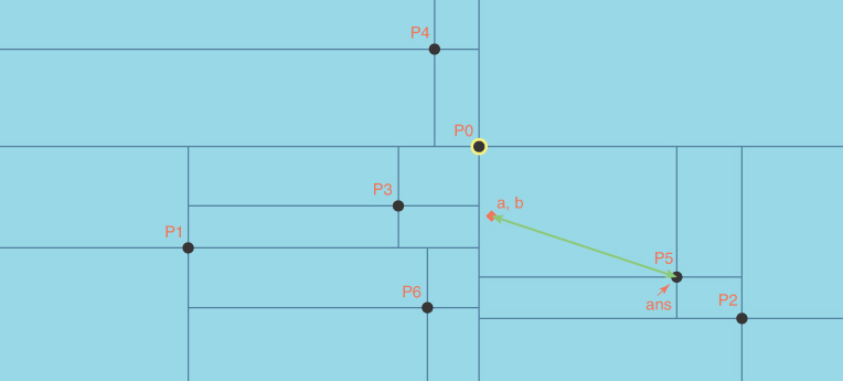
FIGURE 12-27 Finding the nearPoint during a find nearest search
Finding the near point and storing it in ans does not involve any distance calculations, only coordinate comparisons. The findNearest() method then computes the distance from the query point to the ans, as shown by the green line in Figure 12-27. The resulting dist measure is passed to the first call to the __nearest() method as the query circle radius (the distance from the current cand to the query point).
The first call to __nearest() examines the root node, P0. After checking the base cases of visiting an empty leaf node or finding an exact coordinate match where dist is 0, the method measures the distance from P0 to the query point. Figure 12-28 shows this measurement and makes it clear that P0 is closer than the candidate, cand, found by __nearPoint(), P5.

FIGURE 12-28 Visiting the root node during a find nearest search
The visualization tool also displays the various Bounds objects used by __nearest(). Initially, only the bounds value passed as an argument appears and has infinite extent. Figure 12-28 shows the bounds value both at the top right as a string and with diagonal hashing in the same color over the entire display.
The distance from the query point (a, b) to P0 is 62.2, which is less than the dist measure to the cand point shown in the upper left. That means the __nearest() method replaces cand with the current node, P0, and updates the dist measure, reducing the query circle. That new radius is what’s used to compute the circle bounds, cBounds, which is used to determine what quadrants to explore.
Figure 12-29 shows the situation when __nearest() is being called on the southeast child of the root. The n pointer indicates the current node, P2, while cand still points at P0. At this point, three Bounds objects are displayed (in addition to a faded version of the infinite bounds of the root node). The bounds region was passed from the calling routine and covers the whole southeast quadrant of P0. The cBounds region shows the query circle bounding box around a, b. That was made just large enough to include P0, the root and the current best cand point. It’s shown in a different color and with a different angle for the hash marks. Finally, the newB region shows the region currently being checked to see whether it should be searched, P2’s southwest quadrant. It’s displayed in a third color and different hash angle. It’s bounded on three sides by its point’s coordinates and the bounds inherited from its parent, P0. Because newB doesn’t overlap the cBounds region, it’s clear that the southwest quadrant of P2 could not contain any points closer than current best cand point. Thus, the __nearest() method does not make a recursive call for the southwest quadrant of P2. It will, however, make a call for the northwest quadrant of P2 and visit node P5 because that quadrant does overlap the cBounds region.

FIGURE 12-29 Eliminating quadrants during find nearest search
Although the overlapping information in the visualization tool may be confusing, the eliminated quadrants are somewhat easier to see. P2’s SW, NE, and SE quadrants are eliminated, as are P5’s NE and SE, P6’s SW and SE, P1’s NW and SW, P3’s NW and SW, and P4’s NW and NE quadrants. That’s about half of the quadrants, which is similar to how binary search removes half of the range of cells to explore.
Efficiency of findNearest()
The time complexity of findNearest() is on average O(log N). The __nearPoint() method, which behaves similarly to findExact(), should be able to identify a candidate Node in O(log N) time, unless the tree is highly unbalanced. Likewise, a good initial candidate will result in a tight query circle, enabling __nearest() to efficiently descend back down into the tree considering just a small number of adjacent QuadTree cells, again in O(log N) time. An unbalanced tree or a degenerate distribution of data could result in O(N) time for each search. For example, if all the QuadTree nodes are distributed in a circle, and the query point is at or very near the center of the circle. Then, __nearest()has no alternative but to visit every Node in the QuadTree because the search circle necessarily overlaps each nonempty QuadTree cell.
Theoretical Performance and Optimizations
PointList, Grid, and QuadTree present three different approaches to storing and querying spatial data points. Table 12-1 summarizes the average Big O complexity of each operation implemented across spatial data structures.
Table 12-1 Big O Performance of the Spatial Data Structures
PointList | Grid | QuadTree | |
|---|---|---|---|
| O(N) | O(N) | O(log N) |
| O(N) | O(N) | O(log N) |
| O(N) | O(N) | O(log N) |
| O(N) | O(N) | O(log N) |
| O(N) | O(N) | O(N) |
Could the Big O of PointList and Grid be improved to be competitive or superior to QuadTree?
One easy enhancement for PointList would be to use a hash table (such as a Python dictionary) instead of a list to store the entire collection of points in a PointList. Doing so would result in improved O(1) performance for insert(), findExact(), and delete(). The performance of findNearest() and traverse(), however, would not be improved because both require considering every point in the PointList.
The Grid implementation already uses a hash table to map grid cell coordinates to lists of points stored in each grid cell. Because the grid spacing is fixed, however, the list in each grid cell contains O(N) points, making the find and delete methods also O(N). By replacing the list in each grid cell with a dictionary, the performance of findExact() and delete() can also be improved to O(1). Here, too, findNearest() remains O(N) because the nearest neighbor to query point is found by examining all the O(N) points stored in one or more of the grid cells.
Even with these improvements, QuadTree’s theoretical O(log N) performance for findNearest() is difficult to surpass.
Practical Considerations
In this chapter we covered three different ways to organize spatial data: brute force using a list of points, uniform grids, and quadtrees. If you have dozens or even hundreds of spatial data points, then the brute-force approach may be sufficient.
But what should you use if you have many more points—say, tens of thousands, hundreds of thousands, or even millions? Understanding the Big O of a data structure provides some guidance. But remember that the Big O of an algorithm informs you only of the shape of the curve. It (intentionally) excludes an important constant factor that can make a difference in real-life applications.
Let’s examine some practical time measurements of the performance of the Grid and QuadTree data structures. To do this, we ran experiments where we loaded points into a Grid or a QuadTree and then recorded the time to do 1,000 findNearest() queries. Geographic data points were randomly selected with a uniform distribution across a rectangle that roughly encompasses the continental United States. Then 1,000 uniformly distributed query points were randomly selected across that same rectangle, and the time to find the nearest data point was recorded.
Figure 12-30 shows the results of these informative experiments. The X axis shows the number of points loaded into a Grid or QuadTree data structure. The Y axis shows the total time in seconds to run 1,000 findNearest() queries against the data. For grids, we created a Grid object where the cells were sized at 0.5 degrees in latitude and longitude—resulting in about 6,500 grid cells covering the United States. A second grid object was created where the cells were of size 1.0 degrees latitude and longitude—resulting in about 1,600 grid cells. Finally, we also created a QuadTree, also loaded with varying numbers of points, but able to grow in depth as more points were inserted.

FIGURE 12-30 Performance of findNearest() on different-sized data sets
Not surprisingly, the red and blue plot lines are quite linear, confirming the analysis of their O(N) performance. Their slopes reflect the respective sizes of the grid cells and, therefore, how many points are stored on average per cell. In the long run, as the data structures are loaded with millions of points, QuadTrees win, with their very slow O(log N) growth as the number of points increases.
Interestingly, if you have only 100,000 or fewer points, then grids of cell size 1 or 0.5 degrees can perform better than quadtrees. If you were willing to expend more memory on grid cell storage, then an even finer grid would result in better linear performance, by reducing the leading constant factor. Be careful, however, in ensuring that the data won’t grow much larger in software that uses grids like these.
These experiments were somewhat artificial because real-life data is usually not uniformly distributed across the map. Businesses, people, vehicles, and other real-life objects tend to be very clustered in space. If that’s what your data looks like, then you should be especially careful to measure the performance of your spatial data structure under realistic conditions.
Further Extensions
We have explored the basics of spatial data: what it is, how you might organize points in a data structure, and how those organizations impact the four basic operations. The search operation, common to all data structures, needed extensions for exact matches and nearest match. Spatial data, however, is used for many different purposes, and those applications often require more capabilities than what we’ve described here. Let’s explore a few extensions.
Other Operations
Beyond the insert(), findExact(), findNearest(), delete(), and traverse() operations we covered, there are many other possible—and useful—operations on spatial data. Here are just a few:
- Instead of finding just the one nearest neighbor to a point, find the K nearest neighbors to the query point.
- Traverse the points in order of increasing distance from a query point.
- Find all points within a specified distance from a query point.
- Find all points within a rectangular region of space.
- Find all points that lie within a polygonal boundary such as the borders of a country.
- Find the closest pair of points.
Each of these operations needs special algorithms to identify candidate points, determine whether they affect the output, and determine how to incorporate them in the output. Making them efficient is a challenge.
Higher Dimensions
The data structures covered in this chapter all deal with two-dimensional data—points on the plane or on the surface of the globe, specified with just two coordinates. Point data in three dimensions is also common. For example, a third dimension could correspond to the height of an object above the plane or globe. A natural extension to the Grid class could be used to store and query three-dimensional points. In effect, a three-dimensional grid would look like a regularly spaced collection of cubes (instead of squares).
Quadtrees also have a natural analog in the three-dimensional world, namely octrees. With quadtrees, each point recursively subdivides space into four quadrants. With octrees, each point subdivides space into eight octants. Analogous to map data, octrees are efficient at representing and searching three-dimensional point data that clusters in space.
It is possible to use spatial data structures to represent point data in even higher dimensions. You can use k-d trees (that is, k-dimensional) to represent points in arbitrarily high dimensions. These k-d trees are usually implemented by recursively subdividing space into half along carefully chosen dimensions.
These higher dimensional data structures can support the same types of operations, including insert, traverse, find exact, and find nearest.
Implementing and using data structures for high-dimensional data brings theoretical and engineering challenges. In a discussion of the distance between points in two-dimensional and three-dimensional space, you gain an intuitive understanding of what “distance” means. But when you consider additional dimensions, the notion of spatial distance is not meaningful and must be addressed carefully. For example, a fourth dimension of time could be very useful, but then what distance function would be useful in a space consisting of x, y, z, and time?
High-dimensional data also suffers from the “curse of dimensionality.” If you measure the Euclidean distance between two points of very high dimension, the differences in distances among many pairs of points can be very small. Another way to say this is that if you have high-dimensional data, all points in your data set can seem equally or nearly equally distant from each other! Therefore, although quadtrees and even k-d trees for low-dimensional data can be searched in O(log N) time, as the dimension of your data increases, it becomes necessary to search a larger and larger proportion of all the tree’s cells and data points to find a nearest neighbor!
Summary
- Spatial data structures store point data based on two-dimensional position.
- Positions can correspond to Cartesian x, y coordinates, or geographic latitude and longitude coordinates on the Earth.
- Distance between points is measured differently depending on the coordinate systems.
- The Euclidean distance computes the straight-line distance between points on a plane.
- The haversine distance computes the distance along the great circle connecting points on a globe.
- Point data can be stored in different kinds of spatial data structures.
- A brute-force approach stores points in a list or in an array such as the
PointList. - A
Gridstructure divides up the plane or globe into cells of equal size and stores point data as lists or arrays for each cell. - Quadtrees organize point data as a tree.
- Each node in a quadtree stores data for a particular point in space.
- A quadtree node can have up to four child nodes corresponding to the four quadrants relative to its position.
- Grid structures do not adapt to point data that clusters spatially, but quadtrees do.
- All spatial data structures provide methods to insert new point data, search for an exact match, and search for the nearest point data to a query point.
- Grid searches begin in the query point grid cell and expand outward by layer.
- Quadtree searches begin at the root node and follow child quadrants containing the query point.
- Search performance is improved by eliminating grid cells or quadrants that lie outside of the current query circle.
- Query circles have a different shape when geographic coordinates are plotted with parallel lines for longitude meridians as in the Mercator projection.
- Rectangular bounding boxes simplify testing for the intersection or complete enclosure of one region and another but can only approximate the boundary of a query circle.
- Different spatial data structures yield different Big O performance.
- Simple point lists and grids take O(N) time for search and deletion (and insertion when duplicate points must be detected and updated).
- Quadtrees take O(log N) time for insertion, search, and deletion.
- The performance of spatial data structures can be improved by augmenting the structure with O(1) data structures such as hash tables.
- It is important to perform measurements with real-life data for your application to determine the best approach for your scale and type of data.
- Uniformly distributed data can be organized well with grids, and the grid cells can be made small to improve performance.
- Nonuniform data, or data of unknown size or distribution can be better organized with quadtrees because the quadtree adaptively subdivides space in regions that contain more data.
- Octrees can store and search three-dimensional data.
- There are a wide variety of other operations needed for spatial data applications.
Questions
These questions are intended as a self-test for readers. Answers may be found in Appendix C.
1. What distinguishes the keys for spatial data structures from those used for other structures like trees, arrays, and lists?
2. _________ coordinates are used to represent a point on the surface of the earth.
3. When you’re making data structures for two-dimensional spatial data, what things must be initialized when creating the (empty) structure for all of them?
4. Bounding boxes are used in spatial calculations because
a. rectangles are the only viable shapes that work with spatial coordinates.
b. checking whether two rectangles overlap is computationally simpler than checking whether an ellipsoid overlaps with a rectangle.
c. using bounding boxes is a convenient way to put a bound on the worst-case complexity of a spatial computation.
d. the haversine distance works only with rectangular bounds.
5. True or False: Lists of points are never an acceptable data structure for searching spatial data.
6. What advantage does a grid have over a point list in storing spatial data?
7. What advantage does a quadtree have over a grid in storing spatial data?
8. To implement efficient access to the cells of a grid, you use
a. a two-dimensional array or a list to store each cell of the grid containing data points.
b. a quadtree to locate the quadrant storing the cell.
c. a list of point coordinates sorted by each point’s row and column number.
d. a hash table that maps keys consisting of row, column tuples to the list of corresponding points in that grid cell.
9. Using Big O notation, how long does it take to find the nearest neighbor to a query point in each of the following structures holding N points?
a. a point list
b. a grid
c. a quadtree
10. True or False: A quadtree supports data points with any number of dimensions.
11. Query circles
a. are used in find exact searches to determine whether a point matches the query.
b. are used by quadtrees to bound the size of each node’s quadrants.
c. are used by grids to limit which other grid cells should be traversed.
d. start large and decrease in radius as find nearest searches points in grids and quadtrees.
12. True or False: A quadtree uses layers to gradually expand the search for the nearest point.
13. What are the quadrants of a node? How are points lying on the boundary between two quadrants placed into the appropriate quadrant?
14. The depth of a well-balanced quadtree of N points is proportional to
a. N
b. N/4
c.
d. log4 N
15. True or False: Quadtrees are superior because their worst-case behavior is always better than point lists or grids.
Experiments
Carrying out these experiments will help to provide insights into the topics covered in the chapter. No programming is involved.
12-A Which of the three spatial data structures discussed in this chapter would use the least amount of memory per spatial data point? Which would use the most memory for the same number of points?
12-B Consider the problem of finding the item the farthest from a query point. How would you approach this problem, and which data structure would be more appropriate: a grid or a quadtree?
12-C The quadtree makes finding the nearest point very fast. Could the principles used in findNearest() be applied to finding the nearest key in other data structures? More specifically, how could you speed up the search for the nearest key in a binary search tree? Does the answer change if the keys are strings instead of integers?
12-D Consider the problem of finding the K nearest neighbors of a query point. How would you implement this method using your choice of spatial data structure, and what supplementary data structure might you use to make the implementation efficient?
Programming Projects
Writing programs to solve the Programming Projects helps to solidify your understanding of the material and demonstrates how the chapter’s concepts are applied. (As noted in the Introduction, qualified instructors may obtain completed solutions to the Programming Projects on the publisher’s website.)
12.1 Modify the Grid class to support a delete() method that is given the coordinates of a point to delete. If the point is found in the Grid, then the point is deleted from the appropriate cell, and the associated data is returned to the client. If the point is not found, then None is returned to the client.
12.2 Modify the QuadTree class to support a delete() method. Because a Node object can’t easily be removed from a QuadTree, consider adopting the representation that a Node with None for its data denotes a “deleted” node. When implementing delete this way, you must modify the class’s other methods to be consistent with this new representation. If the point is not found, then None is returned to the client.
12.3 Modify Grid and QuadTree to store more than one datum at a specific coordinate. In other words, change them to allow duplicate keys. Be sure to modify all methods that could be impacted by this change.
12.4 Create a subclass of QuadTree called BulkQuadTree. The new subclass has a constructor that accepts a sequence of points in bulk and then attempts to build a well-balanced quadtree. Add measurement methods to the quadtree to quantify its balance and measure the balance of quadtrees using large collections of random points and large collections of sorted points.
12.5 Add a method to Grid that moves the data associated with a point at a specified location to a new location.