Chapter 11
Hash Tables
In This Chapter
Ahash table is a data structure that offers very fast insertion and searching. When you first hear about them, hash tables sound almost too good to be true. No matter how many data items there are, insertion and searching (and sometimes deletion) can take close to constant time: O(1) in Big O notation. In practice this is just a few machine instructions.
For a human user of a hash table, this amount of time is essentially instantaneous. It’s so fast that computer programs typically use hash tables when they need to look up hundreds of thousands of items in less than a second (as in spell checking or in auto-completion). Hash tables are significantly faster than trees, which, as you learned in the preceding chapters, operate in relatively fast O(log N) time. Not only are they fast, hash tables are relatively easy to program.
Despite these amazing features, hash tables have several disadvantages. They’re based on arrays, and expanding arrays after they’ve been allocated can cause challenges. If there will be many deletions after inserting many items, there can be significant amounts of unused memory. For some kinds of hash tables, performance may degrade catastrophically when a table becomes too full, so programmers need to have a fairly accurate idea of how many data items will be stored (or be prepared to periodically transfer data to a larger hash table, a time-consuming process).
Also, there’s no convenient way to visit the items in a hash table in any kind of order (such as from smallest to largest). If you need this kind of traversal, you’ll need to look elsewhere.
However, if you don’t need to visit items in order, and you can predict in advance the size of your database or accept some extra memory usage and a tiny bit of slowness as the database is built up, hash tables are unparalleled in speed and convenience.
Introduction to Hashing
In this section we introduce hash tables and hashing. The most important concept is how a range of key values is transformed into a range of array index values. In a hash table, this transformation is accomplished with a hash function. For certain kinds of keys, however, no hash function is necessary; the key values can be used directly as array indices. Let’s look at this simpler situation first and then go on to look at how hash functions can be used when keys aren’t distributed in such an orderly fashion.
Bank Account Numbers as Keys
Suppose you’re writing a program to access the bank accounts of a small bank. Let’s say the bank is fairly new and has only 10,000 accounts. Each account record requires 1,000 bytes of storage. Thus, you can store the entire database in only 10 megabytes, which will easily fit in your computer’s memory.
The bank director has specified that she wants the fastest possible access to any individual record. Also, every account has been given a number from 0 (for the first account created) to 9,999 (for the most recently created one). These account numbers can be used as keys to access the records; in fact, access by other keys is deemed unnecessary. Accounts are seldom closed, but even when they are, their records remain in the database for reference (to answer questions about past activity). What sort of data structure should you use in this situation?
Index Numbers as Keys
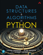
One possibility is a simple array. Each account record occupies one cell of the array, and the index number of the cell is the account number for that record. This type of array is shown in Figure 11-1.
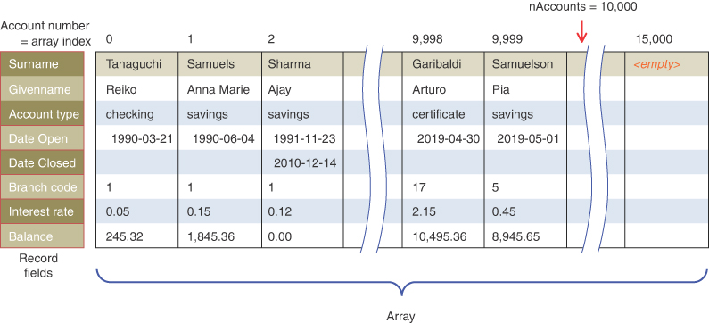
FIGURE 11-1 Account numbers as array indices
As you know, accessing a specified array element is very fast if you know its index number. The clerk looking up what account a check is drawn from knows that it comes from, say, number 72, so he enters that number, and the program goes instantly to index number 72 in the array. A single program statement is all that’s necessary:
accountRec = databaseArray[72]
Adding a new account is also very quick: you insert it just past the last occupied element. If there are currently 9,300 accounts, the next new record would go in cell 9,300. Again, a single statement inserts the new record:
databaseArray[nAccounts] = newAccountRecord()
The count of the number of accounts would be incremented like this:
nAccounts += 1
Presumably, the array is made somewhat larger than the current number of accounts, to allow room for expansion, but not much expansion is anticipated, or at least it needs to be done only infrequently, such as once a month.
Not Always So Orderly
The speed and simplicity of data access using this array-based database make it very attractive. This example, however, works only because the keys are unusually well organized. They run sequentially from 0 to a known maximum, and this maximum is a reasonable size for an array. There are no deletions, so memory-wasting gaps don’t develop in the sequence. New items can be added sequentially at the end of the array, and the array doesn’t need to be much larger than the current number of items.
A Dictionary
In many situations the keys are not so well behaved, as in the bank account database just described. The classic example is a dictionary. If you want to put every word of an English-language dictionary, from a to zyzzyva (yes, it’s a word), into your computer’s memory so they can be accessed quickly, a hash table is a good choice.
A similar widely used application for hash tables is in computer-language compilers, which maintain a symbol table in a hash table (although balanced binary trees are sometimes used). The symbol table holds all the variable and function names made up by the programmers, along with the address (or register) where they can be found in memory. The program needs to access these names very quickly, so a hash table is the preferred data structure.
Coming back to natural languages, let’s say you want to store a 50,000-word English-language dictionary in main memory. You would like every word to occupy its own cell in a 50,000-cell array, so you can access the word’s record (with definitions, parts of speech, etymology, and so on) using an index number. This approach makes access very fast, but what’s the relationship of these index numbers to the words? Given the word ambiguous, for example, how do you find its index number?
Converting Words to Numbers
What you need is a system for turning a word into an appropriate index number. To begin, you know that computers use various schemes for representing individual characters as numbers. One such scheme is the ASCII code, in which a is 97, b is 98, and so on, up to 122 for z.
The extended ASCII code runs from 0 to 255, to accommodate capitals, punctuation, accents, symbols, and so on. There are only 26 letters in English words, so let’s devise our own code, a simpler one that can potentially save memory space. Let’s say a is 1, b is 2, c is 3, and so on up to 26 for z. We’ll also say a blank—the space character—is 0, so we have 27 characters. (Uppercase letters, digits, punctuation, and other characters aren’t used in this dictionary.)
How could we combine the digits from individual letter codes into a number that represents an entire word? There are all sorts of approaches. We’ll look at two representative ones, and their advantages and disadvantages.
Adding the Digits
A simple approach to converting a word to a number might be to simply add the code numbers for each character. Say you want to convert the word elf to a number. First, you convert the characters to digits using our homemade code:
e = 5 l = 12 f = 6
Then you add them:
5 + 12 + 6 = 23
Thus, in your dictionary the word elf would be stored in the array cell with index 23. All the other English words would likewise be assigned an array index calculated by this process.
How well would this approach work? For the sake of argument, let’s restrict ourselves to 10-letter words. Then (remembering that a blank is 0), the first word in the dictionary, a, would be coded by
0 + 0 + 0 + 0 + 0 + 0 + 0 + 0 + 0 + 1 = 1
The last potential word in the dictionary would be zzzzzzzzzz (10 letter z’s). The code obtained by adding its letters would be
26 + 26 + 26 + 26 + 26 + 26 + 26 + 26 + 26 + 26 = 260
Thus, the total range of word codes is from 1 to 260 (assuming a string of all spaces is not a word). Unfortunately, there are 50,000 words in the dictionary, so there aren’t enough index numbers to go around. If each array element could hold about 192 words (50,000 divided by 260), then you might be able fit them all in, but how would you distinguish among the 192 words in one array element?
Clearly, this coding presents problems if you’re thinking in terms of the one word-per-array element scheme. Maybe you could put a subarray or linked list of words at each array element. Unfortunately, such an approach would seriously degrade the access speed. Accessing the array element would be quick, but searching through the 192 words to find the one you wanted could be very slow.
So this first attempt at converting words to numbers leaves something to be desired. Too many words have the same index. Certainly, any anagram of a word would have the same code because the order of the letters doesn’t change the value. In addition, these words
acne ago aim baked cable hack
and dozens of other words have letters that add to 23, as elf does. For words with higher codes, there could be hundreds of other matching words. It is now clear that this approach doesn’t discriminate enough, so the resulting array has too few elements. We need to spread out the range of possible indices.
Multiplying by Powers
Let’s try a different way to map words to numbers. If the array was too small before, make sure it’s big enough. What would happen if you created an array in which every word—in fact, every potential word, from a to zzzzzzzzzz—was guaranteed to occupy its own unique array element?
To do this, you need to be sure that every character in a word contributes in a unique way to the final number.
You can begin by thinking about an analogous situation with numbers instead of words. Recall that in an ordinary multidigit number, each digit-position represents a value 10 times as big as the position to its right. Thus 7,546 really means
7*1,000 + 5*100 + 4*10 + 6*1
Or, writing the multipliers as powers of 10:
7*103 + 5*102 + 4*101 + 6*100
In this system, you break a number into its digits, multiply them by appropriate powers of 10 (because there are 10 possible digits), and add the products. If this happened to be an octal number using the digits from 0 to 7, then you would get 7*83 + 5*82 + 4*81 + 6*80.
In a similar way, you can decompose a word into its letters, convert the letters to their numerical equivalents, multiply them by appropriate powers of 27 (because there are 27 possible characters, including the blank), and add the results. This approach gives a unique number for every word.
Let’s return to the example of converting the word elf to a number. You convert the digits to numbers as shown earlier. Then you multiply each number by the appropriate power of 27 and add the results:
5*272 + 12*271 + 6*270
Calculating the powers gives
5*729 + 12*27 + 6*1
and multiplying the letter codes times the powers yields
3,645 + 324 + 6
which sums to 3,975.
This process does indeed generate a unique number for every potential word. You just calculated a 3-letter word. What happens with larger words? Unfortunately, the range of numbers becomes rather large. The largest 10-letter word, zzzzzzzzzz, translates into
26*279 + 26*278 + 26*277 + 26*276 + 26*275 + 26*274 + 26*273 + 26*272 + 26*271 + 26*270
Just by itself, 279 is more than 7,000,000,000,000, so you can see that the sum will be huge. An array stored in memory can’t possibly have this many elements, except perhaps, in some huge supercomputer. Even if it could fit, it would be very wasteful to use all that memory to store a dictionary of just 50,000 words.
The problem is that this scheme assigns an array element to every potential word, whether it’s an actual English word or not. Thus, there are cells reserved for aaaaaaaaaa, aaaaaaaaab, aaaaaaaaac, and so on, up to zzzzzzzzzz. Only a small fraction of these cells is necessary for real words, so most array cells are empty. This situation is illustrated in Figure 11-2. Near the word elf, there are several words that would be stored, such as elk, eli (for the given name Eli), and elm. The red arrows indicate a pointer to a record describing the word. At other places, such as around the word bird, there would be many unused cells, indicated by the cells without a pointer to some other structure.
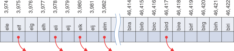
FIGURE 11-2 Index for every potential word
The first scheme—adding the numbers—generated too few indices. This latest scheme—adding the numbers times powers of 27—generates too many.
Hashing
What we need is a way to compress the huge range of numbers obtained from the numbers-multiplied-by-powers system into a range that matches a reasonably sized array.
How big an array are we talking about for this English dictionary? If you have only 50,000 words, you might assume the array should have approximately this many elements. It’s preferable, however, to have extra cells, rather than too few, so you can shoot for an array twice that size, 100,000 cells. We discuss the advantages to having twice the minimum amount needed a little later.
Thus, we seek a way to squeeze a range of 0 to more than 7 trillion into the range 0 to 100,000. A simple approach is to use the modulo operator (%), which finds the remainder when one number is divided by another.
To see how this approach works, let’s look at a smaller and more comprehensible range. Suppose you are trying to squeeze numbers in the range 0 to 199 into the range 0 to 9. The range of the big numbers is 200, whereas the smaller range has only 10. If you want to convert a big number (stored in a variable called largeNumber) into the smaller range (and store it in the variable smallNumber), you could use the following assignment, where smallRange has the value 10:
smallNumber = largeNumber % smallRange
The remainders when any number is divided by 10 are always in the range 0 to 9; for example, 13 % 10 gives 3, and 157 % 10 is 7. With decimal numbers, it simply means getting the last digit. The modulo operation compresses (or folds) a large range into a smaller one, as shown in Figure 11-3. In our toy example, we’re squeezing the range 0–199 into the range 0–9, which is a 20-to-1 compression ratio.
FIGURE 11-3 Range conversion using modulo
A similar expression can be used to compress the really huge numbers that uniquely represent every English word into index numbers that fit in the dictionary array:
arrayIndex = hugeNumber % arraySize
The function that computes the hugeNumber is an example of a hash function. It hashes (converts) a string (or some other piece of data) into a number in a large range. Taking the modulo with the arraySize maps the number into a smaller range. This smaller range is the range of index numbers in an array. The array into which the hashed data is inserted is called a hash table. The index to which a particular key maps is called the hash address. This terminology can be a little confusing. We use the term hash table to describe both the whole data structure and the array inside it that holds items.
To review: you can convert (or encode) a word into a huge number by converting each letter in the word into an integer and then multiplying them by an appropriate power of 27, based on their position in the word. Listing 11-1 shows some Python code that computes the huge number.
LISTING 11-1 Functions to Uniquely Encode Simple English Words as Integers
def encode_letter(letter):         # Encode letters a thru z as 1 thru 26
   letter = letter.lower()         # Treat uppercase as lowercase
   if 'a' <= letter and letter <= 'z':
      return ord(letter) - ord('a') + 1
   return 0                        # Spaces and everything else are 0

def unique_encode_word_loop(word): # Encode a word uniquely using
   total = 0                       # a loop to sum the letter codes times
   for i in range(len(word)):      # a power of 27 based on their position
      total += encode_letter(word[i]) * 27 ** (len(word) - 1 - i)
   return total

def unique_encode_word(word):      # Encode a word uniquely (abbreviated)
   return sum(encode_letter(word[i]) * 27 ** (len(word) - 1 - i)
              for i in range(len(word)))
The encode_letter() function takes a letter, gets its lowercase version, and checks whether it is in the range of 'a' to 'z', inclusive. If it is, it converts the letter to an integer by using Python’s built-in ord() function. This function returns the Unicode value (also called point) of the character, which is the same as the ASCII value for the English letters. It returns the value of the character relative to the 'a' character ensuring that 'a' returns a value of 1. For characters outside the range 'a' to 'z', it returns 0. That means that space is encoded as 0, as well as every other Unicode character that’s not in the range.
To get the unique numeric code for a word, you can use a loop to sum up the values for each letter. The unique_encode_word_loop() function uses an index, i, into the letters of its word parameter to extract each one, get its encoded value using encode_letter(), multiply that value with a power of 27 appropriate for its position, and add the product to the running total. The power of 27 should be 0 for the last character of the word, which has the index len(word) - 1. For the second-to-last character at len(word) - 2, the exponent expression would be 1. The third-to-last would be exponent 2, and so on, up to exponent len(word) - 1 for the first character (leftmost) in the word. After the loop exits, the total is returned.
Listing 11-1 also shows a unique_encode_word() function that computes the exact same encoded value. It calculates it, however, using a more compact syntax with a list comprehension. The sum() function returns the sum of its arguments. The list (tuple) comprehension provides the arguments to sum(). Comprehensions are in the form
expression for variable in sequence
and in the unique_encode_word() function, i is used as the index variable that comes from the comprehension sequence (which are the indices of letters in word). The expression is the same as what was used in the loop version.
The unique_encode_word() function is an example of a hash function. Using the modulo operator (%), you can squeeze the resulting huge range of numbers into a range about twice as big as the number of items you want to store. This computes a hash address:
arraySize = numberWords * 2
arrayIndex = unique_encode_word(word) % arraySize
In the huge range, each number represents a potential data item (an arrangement of letters), but few of these numbers represent actual data items (English words). A hash address is a mapping from these large numbers into the index numbers of a much smaller array. In this array, you can expect that, on the average, there will be one word for every two cells. Some cells will have no words, some will have one, and there can be others that have more than one. How should that be handled?
Collisions
We pay a price for squeezing a large range into a small one. There’s no longer a guarantee that two words won’t hash to the same array index.
This is similar to the problem you saw when the hashing scheme was the sum of the letter codes, but the situation is nowhere near as bad. When you added the letter codes, there were only 260 possible numeric values (for words up to 10 letters). Now you’re spreading the codes over the 100,000 possible array cells.
It’s impossible to avoid hashing several different words into the same array location, at least occasionally. The plan was to have one data item per index number, but this turns out not to be possible in most hash tables. The best you can do is configure things so that not too many words will hash to the same index.
Perhaps you want to insert the word abductor into the array. You hash the word to obtain its index number but find that the cell at that number is already occupied by the word bring, which happens to hash to the exact same number. This situation, shown in Figure 11-4, is called a collision. The word bring has a unique code of 1,424,122, which is converted to 24,122 by taking the modulo with 100,000. The word abductor has the unique code 11,303,824,122, and missable has 139,754,124,122. All three of them hash to index 24,122 of the hash table.
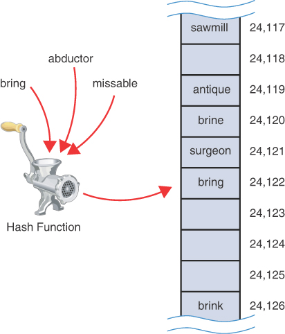
FIGURE 11-4 A collision
The slightly different words brine and brink hash to locations nearby the cell for bring. The reason is that they differ only in their last letter, and that letter’s code is multiplied by 270, or 1. Other words could also hash to those same locations.
How Bad Are Collisions?
Is the hash function a good idea? Could running strings of letters through a “grinder” ever produce some kind of useful hash? It may appear that the possibility of collisions renders the scheme impractical. It would help to know how often they are likely to occur in designing strategies to deal with them.
One relevant measure can be seen by answering a classic question: when is it more likely than not that two people at a gathering share the same birth day and month? Figure 11-5 illustrates the concept. At first, that idea might not seem relevant to hash tables. On closer inspection, you can think of the days in a year as the cells of a hash table. The combined day and month form 366 uniique indices. Each birthday lands in exactly one of them.

FIGURE 11-5 Finding shared birthdays at a gathering
If there are only a few people at the gathering, it’s highly unlikely that they share a birth month and day. If there are 367 people, then it is certain that some have the same birth month and day. Somewhere between those extremes, there’s a number of people where the likelihood of a shared month and day is greater than the likelihood that they are all different.
Maybe intuition tells you that if you have half as many people as there are days in the year, then the likelihood would be greater than 50 percent for a shared birth month and day. In other words, if there are 183 people, it is more likely than not to have a shared birth month and day. That intuition is correct, but the point at which it changes from below 50 percent to above 50 percent is at 23 people. With 22 people, it’s still more likely they all were born on different days. This calculation assumes that the birth days are distributed randomly throughout the year (which is not the case). At a gathering for people born under a particular sign of the zodiac, of course, the distribution would be very different!
So even when the ratio of items to hash table cells is less than 10 percent (23 out of 366), the chance of a collision is greater than 50 percent. That means you should plan your hash tables to always deal with collisions. You can work around the problem in a variety of ways.
We already mentioned the first technique: specifying an array with at least twice as many cells as data items. This means you expect half the cells to be empty. One approach, when a collision occurs, is to search the array in some systematic way for an empty cell and insert the new item there, instead of at the index specified by the hash address. This approach is called open addressing. It’s somewhat like boarding a train or subway car; you enter at one point and take the nearest seat that’s open. If the seats are full, you continue through the car until you find an empty seat. The seat closest to the door where you entered is analogous to the initial hash address.
Returning to hashing words into numbers, if abductor hashes to 24,122, but this location is already occupied by bring, then you might try to insert abductor in cell 24,123, for example. When the insert operation finds an empty cell, it stores both the key and its associated value. In that way, search operations using open addressing can compare the original keys to the keys stored in the table to determine how far the search should continue. It also enables easy checking for empty cells because they won’t have a key-value structure.
A second approach (mentioned earlier) is to create an array that consists of references to another data structure (like linked lists of words) instead of the records for the individual words. Then, when a collision occurs, the new item is simply inserted in the list at that index. This is called separate chaining.
In the balance of this chapter, we discuss open addressing and separate chaining, and then return to the question of hash functions.
So far, we’ve focused on hashing strings. In practice, many hash tables are used for storing strings. Hashing by birthdays is certainly possible, but only useful in rare instances. Many other hash tables are keyed by numbers, as in the bank account number example, or in the case of credit card numbers. In the discussion that follows, we use numbers—rather than strings—as keys. This approach makes things easier to understand and simplifies the programming examples. Keep in mind, however, that in many situations these numbers would be derived from strings or byte sequences.
Open Addressing
In open addressing, when a data item can’t be placed at the index calculated by the hash address, another location in the array is sought. We explore three methods of open addressing, which vary in the method used to find the next vacant cell. These methods are linear probing, quadratic probing, and double hashing.
Linear Probing
In linear probing, the algorithm searches sequentially for vacant cells. If cell 5,421 is occupied when it tries to insert a data item there, it goes to 5,422, then 5,423, and so on, incrementing the index until it finds an empty cell. This operation is called linear probing because it steps sequentially along the line of cells.
The HashTableOpenAddressing Visualization Tool
The HashTableOpenAddressing Visualization tool demonstrates linear probing. When you start this tool, you see a screen like that in Figure 11-6.
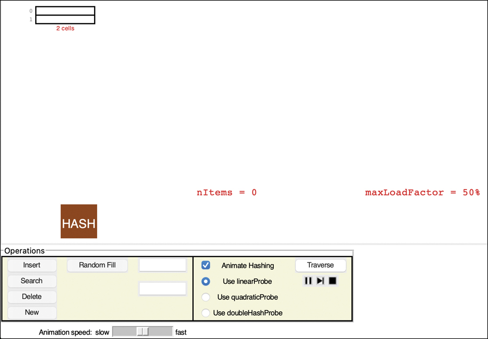
FIGURE 11-6 The HashTableOpenAddressing Visualization tool at startup
In this tool, keys can be numbers or strings up to 8 digits or characters. The initial size of the array is 2. The hash function has to squeeze the range of keys down to match the array size. It does this with the modulo operator (%), as you’ve seen before:
arrayIndex = key % arraySize
For the initial array size of 2, this is
arrayIndex = key % 2
This hash function is simple, so you can predict what cell will be indexed. If you provide a numeric key to one of the operations, the key hashes to itself, and the modulo 2 operation produces either array index 0 or 1. For string keys (anything that contains characters other than the decimal digits), it behaves similar to the unique_encode_word() function shown in Listing 11-1. For example, the key cat hashes to 7627107, which produces index 1. The key bat hashes to one less, 7627106, which produces index 0.
A two-cell hash table can’t hold much data, obviously, and soon you’ll see what happens as it begins to fill up. The number of cells is shown directly below the last cell of the table, and the cell indices appear to the left of each cell. The current number of items stored in the hash table, nItems, is shown in the center.
The box labeled “HASH” represents the hashing function. Let’s see how new keys are processed by it and used to find array indices.
The Insert Button
To put some data in the hash table, type a key, cat for example, in the top text entry box and select Insert. The Visualization tool shows the process of passing the string "cat” through the hashing function to get a big integer. Using the modulo of the table size, it determines a cell index and draws an arrow connecting the hashed result to it like the one shown in Figure 11-7. The arrow points to where probing will begin to find an empty cell. Because the table is initially empty, the first probe finds an empty cell, and the insert operation finishes by copying the key into it—along with a colored background representing some associated data—and then incrementing the nItems value.

FIGURE 11-7 Probing to insert the key cat in an empty hash table
The next item inserted can show what happens in a collision. Inserting the key eat causes a hash address of 7627109, which probes cell 1, as shown in Figure 11-8.
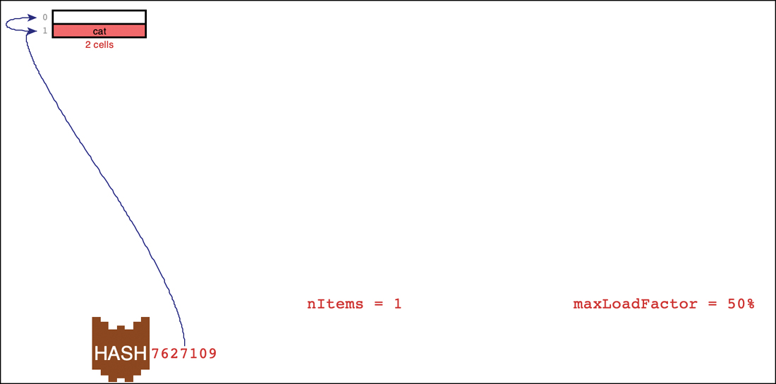
FIGURE 11-8 Probing to insert the key eat
After finding cell 1 occupied, the insertion process begins probing each cell sequentially—linear probing—to find an empty cell, as shown with the additional curved arrow in Figure 11-8. The probing would normally start at index 2, but because that index lies beyond the end of the table, it wraps around to index 0. Because cell 0 is empty, the key eat can be stored there along with its associated data.
After incrementing the nItems value to 2, the table is now full. To be able to add more items in the future, the Visualization tool shows what happens next. A new table is allocated that is at least twice as big. The items from the old table are then reinserted in the new table by rehashing them. The hashing function hasn’t changed, nor have the keys, so it might appear that the items would end up in their same relative positions. Because the size of the table grew, however, the modulo operator produces new cell indices. The cat and eat keys end up in cells 3 and 5 this time, as shown in Figure 11-9.
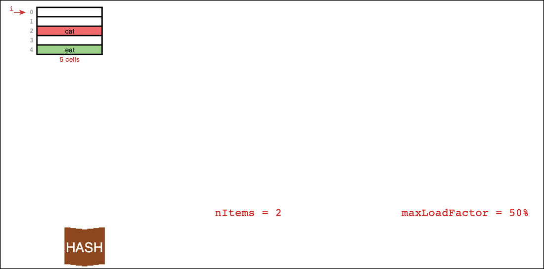
FIGURE 11-9 After inserting cat and eat in an empty hash table
We explore the details of this process in the “Growing Hash Tables” and “Rehashing” sections later. First, let’s explore more about the Visualization tool and linear probing.
The Random Fill Button
Initially, the hash table starts empty and grows as needed. To explore what happens when larger tables become congested, you can fill them with a specified number of data items using the Random Fill button. Try entering 2 in the text entry box and selecting Random Fill. The Visualization tool generates two random strings of characters as keys and animates the process of inserting them.
The animation process takes some time, and when you understand how the insertions work, it may be preferable to jump right to the end result. If you uncheck the button labeled Animate Hashing, the Random Fill operation will perform all the insertions without animation. Similarly, single-item inserts will skip the animation of hashing the key (but not of the probing that happens afterward). Try disabling the animation and inserting 11 more items. You’ll see that as the table grows, it divides into multiple columns, as shown in the example of Figure 11-10.
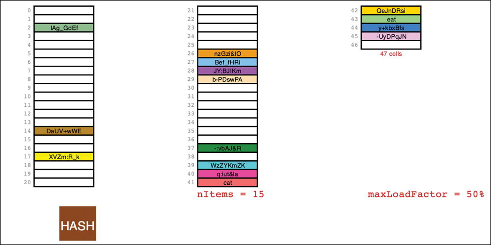
FIGURE 11-10 A hash table with 15 items
The Search Button
To locate items within the hash table, you enter the key of the item and select the Search button. If the Animate Hashing button is checked, the tool animates the conversion of the key string to a large number. The probing of the table begins with the index determined from the hashed key. If it finds the cell filled and the key matches, the key and the color representing its data are copied to an output box.
The Visualization tool simplifies searching for randomly generated and other existing keys by copying the key to the text entry box when a stored key is clicked. The search behavior gets a little more complex when the key isn’t in the table. The tool uses a hashing function that treats numeric keys specially: they hash to their numeric value. Try typing 3 for the key (or clicking the index of another empty cell of a table like the one in Figure 11-10) and selecting Search. The initial probe lands on an empty cell, and the tool immediately discovers that the item is not in the table.
Now try entering the index of a filled cell, like 14 in Figure 11-10. You can also click the index number, but be sure that the key is the numeric index and not the string key stored in the cell. When you select Search, the Visualization tool shows the initial probe going to the selected index. Finding the cell full, but not containing the desired key, it starts linear probing to see whether a collision happened when the item was inserted. The next empty cell probed ends the search.
Filled Sequences and Clusters
As you might expect, some hash tables have items evenly distributed throughout the cells, and others don’t. Sometimes there’s a sequence of several empty cells and sometimes a sequence of filled cells. In the example of Figure 11-10, the filled sequences comprise four 1-item sequences, one 4-item sequence, and one 7-item sequence.
Let’s call a sequence of filled cells in a hash table a filled sequence. As you add more and more items, the filled sequences become longer. This phenomenon is called clustering and is illustrated in Figure 11-11. Note that the order that items were inserted into the table determines how far away a key is placed relative to its default location.

FIGURE 11-11 An example of clustering in linear addressing
When you’re searching for a key, it’s possible that the first indexed cell is already occupied by a data item with some other key. This is a collision; you see the visualization tool add another arrow pointing to the next cell. The process of finding an appropriate cell while handling collisions is called probing.
Following a collision, the hash table’s search algorithm simply steps along the array looking at each cell in sequence. If it encounters an empty cell before finding the goal key, it knows the search has failed. There’s no use looking further because the insertion algorithm would have inserted the item at this cell (if not earlier). Figure 11-12 shows successful and unsuccessful linear probes in a simplified hash table. By simplified, we mean that it uses the last two digits of the key as the table index, which is not a good idea in practice. (You see why a little later.) The initial probe for key 6,378 lands at cell 78. It probes the next adjacent cells until it finds the matching key in cell 81. The search for key 478 also starts at cell 78. After probing 7 cells in the filled sequence, it finds an empty cell at index 85, which ends the search.

FIGURE 11-12 Linear probes in clusters
Try experimenting with filled sequences. Find the starting index of such a sequence like index 26 in Figure 11-10. After clicking that index to copy it into the text entry box, select Insert (not Search). The insertion algorithm must step through all of the filled cells to find the next empty one. After it’s inserted, if you now search for that same index, the search must repeat that same process.
The Delete Button
The Delete button deletes an item whose key is typed by the user. Deletion isn’t accomplished by simply removing a data item from a cell, leaving it empty. Why not? We look at the reason a little later. For now, you can see that the tool replaces the deleted item with a special key that appears as DELETED in the display.
The Insert button inserts a new item at the first available empty cell or in a deleted item. The Search button treats a deleted item as an existing item for the purposes of searching for another item further along.
If there are many deletions, the hash table fills up with these ersatz data items, which makes it less efficient. For this reason, some open addressing hash table implementations don’t allow deletion. If it is implemented, it should be used sparingly to avoid large amounts of unused memory.
Duplicates Allowed?
Can you allow data items with duplicate keys to be used in hash tables? The visualization doesn’t allow duplicates, which is typical behavior for hash tables. As mentioned in previous chapters, this approach implements the storage type as an associative array, where each key can have at most one value.
The alternative of allowing duplicate keys would complicate things. It would require rewriting the search algorithm to look for all items with the same key instead of just the first one, at least in some circumstances. That requires searching through all filled sequences of cells until an empty cell is found. Probing the entire filled sequence wastes time for all table accesses, even when no duplicates are present. Deleting an item would either try to delete the first instance or all instances of a particular key. Both cases require probing filled sequences to find the extent of the duplicates and then moving at least one of the items in the sequence to their default positions if the deletions opened up some cells. For these reasons, you probably want to forbid duplicates or use another data structure if they are required.
Avoiding Clusters
Try inserting more items in the HashTableOpenAddressing Visualization tool. The tool stops growing the table when it reaches 61 cells. As the table gets fuller, the clusters grow larger. Clustering can result in very long probe lengths. This means that accessing cells deeper in the sequence is very slow.
The fuller the array is, the worse clustering becomes. For an extreme example, use the Random Fill button to enter enough random keys so that the total number of keys is 60. Now try searching for a key that’s not in the table. The initial probe lands somewhere in the 61-cell array and then hunts for the single remaining empty (or possibly deleted) cell. If you are unfortunate enough for the initial probe to be the cell after the empty one, the search can go through all 61 cells.
Clustering is not usually a problem when the array is half full and still not too bad when it’s two-thirds full. Beyond this, however, performance degrades seriously as the clusters grow larger and larger. For this reason, it’s critical when designing a hash table to ensure that it never becomes more than half, or at the most two-thirds, full. We discuss the mathematical relationship between how full the hash table is and probe lengths at the end of this chapter.
Clusters are created during insertion but also affect deletion. When an item is deleted from a hash table, you would ideally mark its cell as empty so that it can be used again for a later insert and to break up potential clusters. That simple strategy, however, is a problem for open addressing because probes follow a sequence of indices in the table to locate items, stopping when they find empty cells. If you delete an item that happened to be in the middle of such a sequence, such as item 879 or item 2,578 in Figure 11-12, for example, items landing later in the probe sequence, such as item 6,378, would not be found by subsequent searches. Missing items are particularly problematic when the item being deleted is part of multiple probe sequences. In the example, item 879 happens to be in the probe sequence for item 6,378 even though their sequences start at different table indices.
You might think that there is some way to rearrange items to fill the hole created by a deletion. For instance, what if you follow the probe sequence to its end. Couldn’t you move the last item in the sequence to fill the cell being deleted (somewhat like the successor node replacing a deleted node in a binary search tree)? Unfortunately, that last item in the sequence could be an item with a key that doesn’t hash to the start of the probe sequence used to find the item to be deleted. For example, if you were deleting item 1,078 in Figure 11-12, following its probe sequence to the end would suggest that item 7,184 could replace it, but that would cause that item to be lost from its normal probe sequence that starts at cell 84.
Another idea: what if you find the last item in the deletion probe sequence that shares the same starting cell as the item being deleted? That ensures that you only shift an item on the same probe sequence. Unfortunately, that too causes problems because it could create a new hole in another probe sequence. If some other probe sequence happens to land on the item that was moved, then that sequence is broken. You could try to find any sequences that would visit the cell holding the item being moved as they skipped past collisions, but there could be many, many such sequences. Just like with automobiles, cleaning up after collisions is a big problem.
The approach for deleting items in open addressing is to simply mark cells as deleted, as the Visualization tool shows. The search algorithm can then step past deleted cells as it probes for a key. The insert algorithm, too, can hunt for either empty or deleted cells to use for new items. That helps a bit in keeping the size of clusters small, but only for insertion. You still must search past deleted cells when seeking an item (for search or delete). It also wastes memory, as we discuss later.
Python Code for Open Addressing Hash Tables
Let’s look at the implementation of open addressing in hash tables. Aside from some of the fancier hashing functions, they are straightforward to implement. We’ll make a class where it’s easy to change the hash function and probing technique to resolve collisions. That design choice makes exploring different options more convenient, but it’s not particularly good for performance.
The Core HashTable
The hash table object must maintain an array to hold the items it stores. That table should be private because callers should not be able to manipulate its entries. How big should that table be? We can choose to provide a parameter in the constructor to set the size, but like other data structures, it will be useful to allow it to expand later if more cells are needed.
Because we’re making one class to handle hash tables with different open addressing probes, the constructor also needs a way to specify the method to search when collisions are found. The code in Listing 11-2 handles that feature by providing a probe parameter. The default value for the probe is linearProbe, which we describe shortly. There are also parameters for the initial size of the table, the hash function, and a maxLoadFactor, explained later.
LISTING 11-2 The Core HashTable Class
class HashTable(object):           # A hash table using open addressing
   def __init__(                   # The constructor takes the initial
         self, size=7,             # size of the table,
         hash=simpleHash,          # a hashing function,
         probe=linearProbe,        # the open address probe sequence, and
         maxLoadFactor=0.5):       # the max load factor before growing
      self.__table = [None] * size # Allocate empty hash table
      self.__nItems = 0            # Track the count of items in the table
      self.__hash = hash           # Store given hash function, probe
      self.__probe = probe         # sequence generator, and max load factor
      self.__maxLoadFactor = maxLoadFactor

   def __len__(self):              # The length of the hash table is the
      return self.__nItems         # number of cells that have items

   def cells(self):                # Get the size of the hash table in
      return len(self.__table)     # terms of the number of cells

   def hash(self, key):            # Use the hashing function to get the
      return self.__hash(key) % self.cells() # default cell index
The constructor creates a private __table of the specified size. The initial None value in the cells indicates that they are empty. The count of stored items, __nItems, is set to zero. When items are inserted, they place (key, value) tuples in the table’s cells, making empty and full cells easy to distinguish. All of the rest of the constructor parameters are stored in private fields for later use.
The HashTable defines a __len__() method so that Python’s len() function can be used on instances to find the number of items they contain. A separate cells() method returns the number of cells in the table, so you can see how full the table is by comparing it to the number of items. As it fills, the likelihood of collisions increases.
The other core method shown in Listing 11-2 is the hash() method. This method is used to hash keys into table indices. We’ve allowed the caller to provide the hashing function in the constructor. This could be the unique_encode_word() function from Listing 11-1 or something similar. Whatever function is used, it should return an integer from a single key argument. The modulo of that integer with the number of cells in the table provides the initial table index for that key. This design allows callers to provide hashing functions that return very large integers, which are then mapped to the range of cells in the table.
The simpleHash() Function
The default hash function for the HashTable is simpleHash(), which is shown in Listing 11-3. This function accepts several of the common Python data types and produces an integer from their contents. It’s not a sophisticated hashing function, but it serves to show how such functions are created to handle arbitrary data types.
LISTING 11-3 The simpleHash() Method
def simpleHash(key):                    # A simple hashing function
   if isinstance(key, int):             # Integers hash to themselves
      return key
   elif isinstance(key, str):           # Strings are hashed by letters
      return sum(                       # Multiply the code for each letter by
         256 ** i * ord(key[i])         # 256 to the power of its position
         for i in range(len(key)))      # in the string
   elif isinstance(key, (list, tuple)): # For sequences,
      return sum(                       # Multiply the simpleHash of each element
         256 ** i * simpleHash(key[i])  # by 256 to the power of its
         for i in range(len(key)))      # position in the sequence
   raise Exception(                     # Otherwise it's an unknown type
      'Unable to hash key of type ' + str(type(key)))
The simpleHash() function checks the type of its key argument using Python’s isinstance() function. For integers, it simply returns the integer. Returning the unmodified key is, in general, a very bad idea because many applications use a hash table on integers in a small range. That small range (or distribution) of numbers will map directly to a small range of cell indices in the table and likely cause collisions. We choose to use it here to simplify the processing, experiment with collisions, and look at ways to avoid them.
If the key passed to simpleHash() is a string, the resulting integer it produces is something like the unique_encode_word() function you saw earlier. It takes the numeric value of each character in the key using ord() and multiplies that by a power of 256. The power is the position of the character in the string. The first character is power 0, which multiplies its numeric ord value by 1. The second character gets power 1, so it is multiplied by 2561, the third character is multiplied by 2562, and so on (which is the reverse of the unique_encode_word() function). The multiplication scheme ensures that anagram strings like "ant” and "tan” will map to different values, at least for simple strings. The products are all summed together using sum() and a tuple comprehension.
Note that the use of powers of 256 in the simpleHash() method is not sufficient to distinguish all string values. Because Python strings may contain any Unicode character whose numeric value can range up to 0x10FFFF = 1,114,111, the simpleHash() function can hash different strings to the same integer. Using 1,114,112 as the base instead of 256 avoids that problem, but we use 256 to keep the numbers smaller in our examples at the risk of causing more collisions.
The last elif clause in simpleHash() handles lists and tuples. These are the simple sequence types in Python. They are like strings, except that their elements could be any other kind of data, not just Unicode characters. It applies the same multiplication scheme by recursively calling simpleHash() on the elements individually. In this way, simpleHash() can recursively descend through a complex structure of sequences to find the integers and strings they contain, and build a number based on them and their relative positions.
Finally, if none of the data type tests succeed, simpleHash() gives up and raises an exception to signal that it doesn’t have a method to convert it to an integer.
The search() Method
The search() method is used to find items in the hash table, navigating past any collisions. It does this by calling an internal __find() method to get the table index for the key as shown in Listing 11-4. It’s best to keep that method private because callers shouldn’t need to know which cell holds a particular item.
The __find() method returns an integer index to a cell or possibly None when it cannot find the key being sought. The search() method looks at the returned index and returns None in the cases where the key wasn’t found. In other words, if the index returned by __find() is None or the table cell it indicates contains None, or the key stored in that table cell is not equal to the key being sought, the search for the key failed. The only other possibility is that the table cell’s key matches the one being sought, so it returns the second item in the cell’s tuple, the value associated with the key.
The definition of the constant, __Deleted, might seem a little unusual. This is the value stored in table cells that have been filled and later deleted. It’s a marker value. By making it a tuple in Python, it has a unique reference address that can be compared using the is operator. The code must distinguish between empty cells containing None, deleted cells containing __Deleted, and full cells during open address searching. The comparison test in the __find() method (described shortly) uses the is operator instead of the == operator to compare cell contents with __Deleted in case some application decided to store a copy of that same tuple. The search() method doesn’t care whether the cell returned by __find() is empty or deleted, but the insert() method does, as you see shortly. Note also that the __Deleted marker’s key, None, cannot be hashed by simpleHash(). If it could, then the search() method might return the deleted marker value as a result.
LISTING 11-4 The search() and __find() Methods of HashTable
class HashTable(object):                 # A hash table using open addressing
…
   def search(self,                      # Get the value associated with a key
              key):                      # in the hash table, if any
      i = self.__find(key)               # Look for cell index matching key
      return (None if (i is None) or     # If index not found,
              self.__table[i] is None or # item at i is empty or
              self.__table[i][0] != key  # it has another key, return
              else self.__table[i][1])   # None, else return item value

   __Deleted = (None, 'Deletion marker') # Unique value for deletions

   def __find(self,                      # Find the hash table index for a key
              key,                       # using open addressing probes. Find
              deletedOK=False):          # deleted cells if asked
      for i in self.__probe(self.hash(key), key, self.cells()):
         if (self.__table[i] is None or  # If we find an empty cell or
             (self.__table[i] is HashTable.__Deleted and # a deleted
              deletedOK) or              # cell when one is sought or the
             self.__table[i][0] == key): # 1st of tuple matches key,
            return i                     # then return index
      return None                        # If probe ends, the key was not found
The __find() method takes the search key as a parameter with an optional flag parameter, deletedOK, that indicates whether it can stop after finding a deleted cell. This method implements the core of the open addressing scheme. The key is hashed using the hash function that was provided when the table was created. The hash() method (Listing 11-2) is called to map the large integer computed by simpleHash() or some other hash function to an integer in the range of the current size of the hash table. That hash address is the starting point for probing the cells of the table for the item.
The hash address returned by the call to hash() is passed to the probe function that was given when the hash table was constructed. The loop
for i in self.__probe(self.hash(key), key, self.cells()):
shows that the probe function is being used as a generator. In other words, it must create an iterator that iterates over a sequence. The elements of the sequence are the table cell indices that should be probed for the item. The call to self.hash(key) returns the first index, and the key and number of cells arguments allow the generator to know how to create the rest of the sequence. We look at the linearProbe() generator definition shortly, but first let’s look at the rest of the __find() method.
Inside the for loop, __find() checks the contents of cell i to see what’s stored there. If it’s None, the cell is empty and i can be returned to indicate the key is not in the table. If the cell isn’t empty and has a matching key, then __find() can also return i as the result to indicate the item was found. The only tricky case is what to do if the cell has been marked as deleted. The default (deletedOK=False) is to treat it like another filled cell caused by a collision and continue the probe sequence. Only if the caller asked to stop on deleted cells, and the cell’s value is the __Deleted marker, will __find() end the loop and return.
When some other item is found at cell i, the probe sequence continues. For linear probing, that is just index i+1 or 0, after it reaches the number of cells in the table. If the whole probe sequence is completed without finding any empty cells, then the table must be full of nonmatching or deleted items. It that case, __find() returns None.
The insert() Method
The process of inserting items in the table follows the same scheme as searching and adds a few twists for handling the increasing number of items. Listing 11-5 shows the insert() method getting the index of a cell, i, by calling __find() on the key of the item to insert. The call is made with deletedOK=True to allow finding deleted cells, which insert() will fill.
The first test on i checks whether it is None, indicating that the probe sequence ended without finding the key, an empty cell, or a deleted cell. Either the table is full, or the probe sequence has failed to find any available cells in this case. The insert() method raises an exception for that. The method could try increasing the table size for this situation, but if there’s a problem with the probe sequence, increasing the table size may only make matters worse.
The next test checks whether cell i is empty or deleted. In those cases, the contents can be replaced by a (key, value) tuple to store the item in the cell. Doing so adds a new item to the table, and the insert() method increments the number of items field. That increase could make the table full or nearly full. To reduce the problem of collisions, the method should increase the size of the table when the number of items exceeds some threshold.
What threshold should be used? An absolute number doesn’t make sense because when it’s surpassed, the table could become full again. Instead, it’s better to look at the load factor, the ratio (or percentage) of the table cells that are full. The load_factor() method computes the value, which is always a number in the range 0.0 to 1.0. By comparing the load factor to the maxLoadFactor specified when the hash table was constructed, we can use a single threshold that’s valid no matter how large the hash table grows. We examine the __growTable() method shortly.
LISTING 11-5 The insert() and __growTable() Methods
class HashTable(object):              # A hash table using open addressing
…
   def insert(self,                   # Insert or update the value associated
              key, value):            # with a given key
      i = self.__find(                # Look for cell index matching key or an
         key, deletedOK=True)         # empty or deleted cell
      if i is None:                   # If the probe sequence fails,
         raise Exception(             # then the hash table is full
            'Hash table probe sequence failed on insert')
      if (self.__table[i] is None or  # If we found an empty cell, or
          self.__table[i] is HashTable.__Deleted): # a deleted cell
         self.__table[i] = (          # then insert the new item there
            key, value)               # as a key-value pair
         self.__nItems += 1           # and increment the item count
         if self.loadFactor() > self.__maxLoadFactor: # When load
            self.__growTable()        # factor exceeds limit, grow table
         return True                  # Return flag to indicate item inserted

      if self.__table[i][0] == key:   # If first of tuple matches key,
         self.__table[i] = (key, value) # then update item
         return False                 # Return flag to indicate update

   def loadFactor(self):              # Get the load factor for the hash table
      return self.__nItems / len(self.__table)

   def __growTable(self):             # Grow the table to accommodate more items
      oldTable = self.__table         # Save old table
      size = len(oldTable) * 2 + 1    # Make new table at least 2 times
      while not is_prime(size):       # bigger and a prime number of cells
         size += 2                    # Only consider odd sizes
      self.__table = [None] * size    # Allocate new table
      self.__nItems = 0               # Note that it is empty
      for i in range(len(oldTable)):  # Loop through old cells and
         if (oldTable[i] and          # insert non-deleted items by re-hashing
             oldTable[i] is not HashTable.__Deleted):
            self.insert(*oldTable[i]) # Call with (key, value) tuple
The insert() method finishes by returning True when an empty or deleted cell becomes filled. This value indicates to the caller that another cell became full. The alternative, when the hash table already has a value associated with the key to be inserted, is to replace or update the value with the new one. The final if clause of the insert() method returns False to indicate that no unused cells were filled by the insertion.
Growing Hash Tables
The __growTable() method in Listing 11-5 increases the size of the array holding the cells. We explored growing arrays in one of the Programming Projects from Chapter 2, “Arrays,” and the process is a bit more complicated for hash tables. First, let’s look at how much it should grow. We could add a fixed amount of cells or multiply the number of cells by some growth factor. Adding a small, fixed number of cells would keep the number of unused cells to a minimum. Multiplying by, say 2, creates a large number of unused cells initially, but means that the grow operation will be performed many fewer times.
To see the difference the growth method has, let’s assume that the application using the hash table chooses to start with a small hash table of five cells and that it must store 100,000 key-value pairs. If the choices are to grow the table by five more cells or double its size for each growth step, how many steps will be needed? Table 11-1 shows the steps in growing the size of the table for the two methods.
Table 11-1 Growing Tables by a Fixed Increment and by Doubling
Fixed Size Growth | Doubling Size Growth | |||
|---|---|---|---|---|
Step | Size | Step | Size | |
0 | 5 | 0 | 5 | |
1 | 10 | 1 | 10 | |
2 | 15 | 2 | 20 | |
3 | 20 | 3 | 40 | |
4 | 25 | 4 | 80 | |
… | … | |||
N | 5 * (N +1) | N | 5 * 2N | |
… | … | |||
14 | 75 | 14 | 81,920 | |
15 | 80 | 15 | 163,840 | |
… | ||||
19,998 | 99,995 | |||
19,999 | 100,000 | |||
The fixed size growth takes 20,000 steps to reach the 100,000 cells needed. When the size doubles at every step, the 100,000 capacity is reached on the 16th step. As you’ve seen before, that is the difference between O(N) and O(log N) steps. Reducing the number of growth steps is important because of what must be done after growing the array. Before we look at that, however, there’s another factor in choosing the size of the new array.
The __growTable() method in Listing 11-5 first sets oldTable to reference the current hash table and estimates the size of the next table to be twice the old size, plus one. Then it starts a loop that finds the first prime number that equals or exceeds that size. Why? That’s because prime numbers have special importance with algorithms that use the modulo operator. When you choose a prime number for the size, only multiples of that prime number hash to cell 0. Similarly, only multiples of that prime number plus one hash to cell 1. If the keys to be inserted in the hash table do not have that prime number as a factor, they tend to hash over the whole range of cells. That’s very desirable behavior, as you will see later.
The test for prime numbers, is_prime(), is not a part of standard Python. There are many published algorithms for this (deceptively simple) test, so we don’t show it here.
Rehashing
After deciding the new size of the hash table, the __growTable() method in Listing 11-5 creates the new array and sets the number of items back to zero. That might seem odd; why would we want an empty hash table at this point? The reason is that the key-value pairs in oldTable need to be stored in the new table, but in new positions, and none of them are in place yet. If you simply copy the contents of a cell in oldTable to the cell with the same index in the new array, the __find() method might not find it. The new array size affects where the algorithm starts its search because it is used in the modulo operation that computes the hash address. For example, in Figure 11-12, the linear probe for key 6,378 started at cell 78 and eventually found the item in cell 81 due to collisions. That was when the array size was 100. If the array size is 200, the linear probe would start at cell 178 (6,378 modulo 200). Storing that item at cell 78 in the new table would work only if there were a large cluster extending from 178 through cell 199 and then wrapping around from 0 to 78.
Instead of copying, key-value pairs must be reinserted, a process called rehashing, to ensure proper placement. The insertion process distributes them to their new cells, perhaps causing collisions, but probably fewer collisions than occurred in the smaller array. The __growTable() method in Listing 11-5 loops over all the cells in the smaller array and reinserts any filled cells that are not simply the deleted cell marker. This operation can be quite time-consuming, and it must scan all the cells using the range(len(oldTable)) iterator, not just the __nItems known to be filled.
One implementation note: the asterisk in the self.insert(*oldTable[i]) expression tells Python to take the tuple stored at oldTable[i] and use its two components as the two arguments in the call to insert(), which are key and value. The asterisk (*) means multiplication in most contexts but has a different meaning when it precedes the arguments of a function call or the elements of any tuple.
The linearProbe() Generator
Let’s return to the part of the insert process that probes for empty cells. The __find() method in Listing 11-4 has a loop of the form
for i in self.__probe(self.hash(key), key, self.cells()):
This is the place where the __probe attribute of the object is called to generate the sequence of indices to check. The default value for the __probe attribute is linearProbe(), which is shown in Listing 11-6.
LISTING 11-6 The linearProbe() Generator for Open Addressing
def linearProbe(               # Generator to probe linearly from a
      start, key, size):       # starting cell through all other cells
   for i in range(size):       # Loop over all possible increments
      yield (start + i) % size # and wrap around after end of table
The linearProbe() is a straightforward generator that behaves similarly to Python’s range() generator. In fact, it uses range() in an internal loop that steps a variable, i, through all size cells of the table. The i index is added to the starting index for the probe, so it will examine all the subsequent cells in the array. When that offset index goes past the end of the table, the iterator wraps the index back to zero by using the modulo of the offset index with size. The new index will always be between zero and one less than size.
The yield statement in the loop body sends the new index back to the __find() method to be checked (Listing 11-4). Remember that the yield statement returns a value and control to the caller. The caller then uses the value in its own loop until it’s time to get the next value from the iterator. Control then passes back to the iterator right after the yield statement. In this case, linearProbe() goes on and increments its own i variable.
When linearProbe() finishes going through all the indices of the array, the generator ends (by raising a StopIteration exception). That signals to the caller, __find(), that all the cells have been probed. If the insert() method hasn’t found an empty cell before the linear probe sequence finishes, then the table must be full.
Note that the linearProbe() iterator does not use the goal key to determine the sequence of indices. We will discuss that shortly.
The delete() Method
Deleting items is straightforward for hash tables because you only need to mark the deleted cells. Like with insertion, the delete() method starts by using the __find() method to find the cell containing the item to delete, as shown in Listing 11-7. After the cell index, i, is determined, the behavior depends on what is stored at the cell. If __find() could not discover that cell, or it already contains a deleted element or some other item whose key does not match, then a possible error has been found. This delete() method has an optional parameter, ignoreMissing, which determines whether an exception should be raised. In general, data structures that store and retrieve data should raise exceptions when the caller tries to remove an item not in the store, but in some circumstances such errors can be safely ignored.
LISTING 11-7 The delete() Method of HashTable
class HashTable(object):              # A hash table using open addressing
…
   def delete(self,                   # Delete an item identified by its key
              key,                    # from the hash table. Raise an exception
              ignoreMissing=False):   # if not ignoring missing keys
      i = self.__find(key)            # Look for cell index matching key
      if (i is None or                # If the probe sequence fails or
          self.__table[i] is None or  # cell i is empty or
          self.__table[i][0] != key): # it's not the item to delete,
         if ignoreMissing:            # then item was not found. Ignore it
            return                    # if so directed
         raise Exception(             # Otherwise raise an exception
           'Cannot delete key {} not found in hash table'.format(key))

      self.__table[i] = HashTable.__Deleted # Mark table cell deleted
      self.__nItems -= 1              # Reduce count of items
When the delete() method finds a cell with a matching key, it marks the cell with the special __Deleted marker defined for the class and decrements the count of the number of stored items. Typically, no attempt to resize the hash table is made when many deletions cause the load factor to shrink below the threshold used to determine when to grow the table. Skipping the resize operation is based two assumptions: that deletion will occur much less often than insertion and search, and that the cost of having to rehash all the items stored in the table.
The traverse() Method
To traverse all the items in a hash table, all the table cells must be visited to determine which ones are filled. The process is easy to implement as a generator. The one special consideration is that deleted items should not be yielded. Listing 11-8 shows the implementation.
LISTING 11-8 The traverse() Method of HashTable
class HashTable(object):                 # A hash table using open addressing
…
   def traverse(self):                   # Traverse the key, value pairs in table
      for i in range(len(self.__table)): # Loop through all cells
         if (self.__table[i] and         # For those that contain undeleted
             self.__table[i] is not HashTable.__Deleted): # items
            yield self.__table[i]        # yield them to caller
Because the implementation stores the key-value pairs as (immutable) Python tuples, they can be yielded directly to the caller, which can assign them to two variables in a loop such as
for key, value in hashTable.traverse():
Alternatively, callers can use a single loop variable holding the pair as a tuple.
The Traverse and New Buttons
Returning to the Visualization tool, the Traverse button launches the preceding loop. Each item’s key is printed in a box (ignoring its data and adding a comma to separate the keys). It illustrates the traverse() iterator skipping over empty and deleted cells.
You can create new, empty hash tables with the New button. This button takes two arguments: the number of initial cells and the maximum load factor. You can specify starting sizes of 1 to 61 cells and maximum load factors from 0.2 to 1. When invalid arguments are provided, the default values of 2 and 0.5 are used.
If you create hash tables with nonprime sizes, they will grow using the __growTable() method of Listing 11-5, setting the new size to a prime number. Try stepping through the animation of the rehashing process. This animation shows how the items move to their new cells.
If you want to see the effects of using different table sizes, try using the New button to create a table of the desired size with a maximum load factor of 0.99. The table will not grow until it becomes completely full, so you can see the effects of different table sizes and clustering.
Quadratic Probing
Using open addressing, hash tables can find empty (and deleted) cells to fill with new values, but clusters can form. As clusters grow in size, it becomes more likely that new items will hash to cells within a cluster. The linear probe steps through the cluster and adds the new item to the end, making it even bigger, perhaps joining two clusters.
This behavior is somewhat like that of automobiles entering a highway. If only isolated vehicles make up the flow of highway traffic, the arriving vehicles have plenty of gaps to fit into. When the highway is crowded, longer chains of vehicles form clusters. Newly arriving vehicles wait for the cluster to pass and join at the end, increasing the cluster size. Hopefully, the arriving vehicles don’t cause real-world collisions as they “probe” for an open spot on the highway.
The likelihood of forming clusters and the size of clusters depend on the ratio of the number of items in the hash table to its size—its load factor. Clusters can form even when the load factor isn’t high, especially when the hashing function doesn’t distribute keys uniformly over the table. Parts of the hash table may consist of big clusters, whereas others are sparsely populated. Clusters reduce performance.
Quadratic probing is an attempt to keep clusters from forming. The idea is to probe more widely separated cells instead of those adjacent to the primary hash site.
The Step Is the Square of the Step Number
In a linear probe, if the primary hash index is x, subsequent probes go to x + 1, x + 2, x + 3, and so on. In quadratic probing, subsequent probes go to x + 1, x + 4, x + 9, x + 16, x + 25, and so on. The distance from the initial probe is the square of the step number: x + 12, x + 22, x + 32, x + 42, x + 52, and so on. Figure 11-13 shows some quadratic probes.
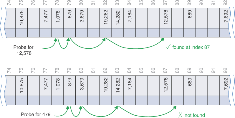
FIGURE 11-13 Quadratic probes
The quadratic probe starts the same as the linear probe. When the initial probe lands on a nonmatching key, it picks the adjacent cell. If that’s occupied, it may be in a small cluster, so it tries something four cells away. If that’s occupied, the cluster could be a little larger, so it tries nine cells away. If that’s occupied, it really starts making long strides and jumps to 16 cells away. Pretty soon, it will go past the length of the array, although it always wraps around because of the modulo operator.
Using Quadratic Probing in the Open Addressing Visualization Tool
The HashTableOpenAddressing Visualization tool can demonstrate different kinds of collision handling—linear probing, quadratic probing, and double hashing. (We look at double hashing in the next section.) You can choose the probe method whenever the table is empty by selecting one of the three radio buttons. When the table has one or more items, the buttons are disabled to preserve the integrity of the data.
To see quadratic probing in action, try the following. Use the New button to create a hash table of 21 cells with a maximum load factor of 0.9. Select the Use quadraticProbe button to switch to quadratic probing. Then use the Random Fill button to insert 12 random keys in the table. This action produces a table with various filled sequences, like the one shown in Figure 11-14. There is a six-cell filled sequence along with several shorter ones.

FIGURE 11-14 Quadratic probing in the HashTableOpenAddressing Visualization tool
In this example, try inserting the key 0. Because it is a numeric key, the hashed value is 0 and the first probe is to cell 0. After finding cell 0 full, it tries the cell at 0 + 1. That cell is occupied, so it continues to cell 0 + 4, finding another stored item. When it reaches 0 + 9, it finds cell 9 empty and can insert key 0 there. It’s easy to see how the quadratic probes spread out further and further.
If you next try to insert the key 21, it will hash to cell 0 for its initial probe again because the table has 21 cells. The insertion now will repeat the same set of probes as for key 0 and then continue on to locate an empty cell. Perhaps surprisingly, it revisits some of the same cells during the probing, as shown in Figure 11-15.
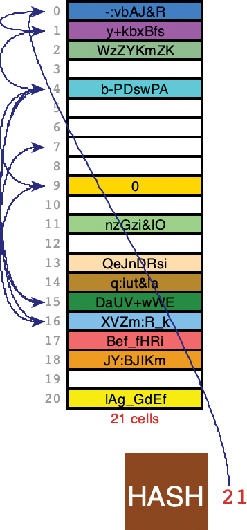
FIGURE 11-15 Inserting key 21 by quadratically probing a relatively full hash table
Specifically, the cells probed to insert key 21 are 0, 1, 4, 9, 16, (25) 4, (36) 15, (49) 7. The indices in parentheses are the values before taking the modulo with 21.
This example is particularly troublesome. Not only does it have to probe all the cells probed to insert key 1, but it also repeats the probe at cell 4 that wouldn’t have occurred using linear probing. If you keep inserting more keys, you will see how this behavior becomes worse when the table is almost full. With the max load factor set to 0.9, it won’t grow the table until the 19th key is inserted.
Incidentally, if you try to fill the hash table up to the maximum 61 items it supports or with a very high maximum load factor, the Visualization tool may not be able to insert an item, even if empty cells remain. The program tries only 61 probes before giving up (or whatever the size of the current table is). Because quadratic probes can revisit the same cells, the sequence may never land on one of the few remaining empty cells.
Also try some searches when the table is nearly full, both for existing keys and ones not in the table. The probe sequences get very long in some cases.
Implementing the quadratic probe is straightforward. Listing 11-9 shows the quadraticProbe() generator. Like the linearProbe() shown in Listing 11-6, it uses range() to loop over all possible cells one time. The loop variable, i, is squared, added to the start index, and then mapped to the possible indices using the modulo operator. Because i starts at zero, the first yielded index is the start index.
LISTING 11-9 The quadraticProbe() Generator for Open Addressing
def quadraticProbe(                 # Generator to probe quadratically from a
      start, key, size):            # starting cell through all other cells
   for i in range(size):            # Loop over all possible cells
      yield (start + i ** 2) % size # Use quadratic increments
The Problem with Quadratic Probes
Quadratic probes reduce the clustering problem with the linear probe, which is called primary clustering. Quadratic probing, however, suffers from different and more subtle problems. These problems occur because all the probing sequences follow the same pattern in trying to find an available cell.
Let’s say 184, 302, 420, and 544 all hash to address 7 and are inserted in this order. Then 302 will require a one-cell offset, 420 will require a four-cell offset, and 544 will require a nine-cell offset from the first probe. Each additional item with a key that hashes to 7 will require longer probes. Although the cells are not adjacent in the hash table, they still are causing collisions. This phenomenon is called secondary clustering.
Secondary clustering is not a serious problem. It occurs for any hashing function that places many keys at the same initial cell or at multiple cells that happen to be spaced by a square number away from other filled cells. There’s another issue, however, and that’s the coverage of cells visited by the probing sequence.
The quadratic probe keeps making larger and larger steps. There’s an unexpected interaction between those steps and the modulo operator used to map the index onto the available cells. In the linear probe, the index is always incremented by one. That means that linear probing will eventually visit every cell in the hash table after wrapping around past the last index.
In quadratic probing, the increasing step sizes mean that it eventually visits only about half the cells. The example in Figure 11-15 illustrated part of the problem when it revisited cell 4. The reason for this behavior takes some mathematics to explain.
If you look at the spacing between the cells probed, you’ll see that it increases by two at each step. The spacing between x + 1 and x + 4 is three. The spacing between x + 4 and x + 9 is five. The spacing between x + 9 and x + 16 is seven, and so on. It already looks as though it might skip every other cell because it will stay on the odd cells if the initial probe was to an even cell (and vice versa). That’s actually not the case because the modulo operator will change between odd and even numbered cells when the index goes past the modulo value. That value is usually a prime number, so it is odd.
Even with a prime number of cells, however, the quadratic probe starts repeating the same sequence of cell indices fairly quickly. Here’s a basic example. For simplicity, let’s say the hash table has seven cells in it, and the key to store initially hashes to cell index 0. Quadratic probing then visits indices 1, 4, 9, 16, 25, 36, 49, 64, and so on. After taking the modulo with seven, however, the full sequence is 0, 1, 4, 2, 2, 4, 1, 0, 1, 4, 2, 2, 4, 1, 0, and so on. That 0, 1, 4, 2, 2, 4, 1 sequence repeats forever, leaving out cell indices 3, 5, and 6.
Three cells may not seem like much, but they’re three out of seven cells total. Even worse, the probe revisits indices 1, 2 and 4 twice. Because they’ve already been visited during the seven-probe sequence, they must already be occupied, so revisiting them just wastes time (much more time than the single cell revisited in the example in Figure 11-15). As the prime number of cells gets bigger, the repetitive behavior continues. After the quadratic term grows to be the square of the table size, the sequence returns to the starting index. Eventually, about half of the cells are visited, and half are not.
So linear probing ends up causing primary clustering, whereas quadratic probing ends up with secondary clustering and only half the coverage of the hash table. This approach is not used because there’s a much better solution.
Double Hashing
To eliminate secondary clustering as well as primary clustering and to help with hash table coverage, there’s another approach: double hashing. Secondary clustering occurs for any algorithm that generates the same sequence of probing for every key.
What we need are probe sequences that differ for each key instead of being the same for every key. Then numbers with different keys that hash to the same index will use different probe sequences.
The double hashing approach hashes the key a second time, using a different method, and uses the result as the step size. For a given key, the step size remains constant throughout a probe, but it’s different for different keys. As long as the step size is not a multiple of the array size, it will eventually visit all the cells. That’s one reason why prime numbers are good for the array size; they make it easier to avoid getting a step size that evenly divides the size of the array.
Experience has shown that this secondary hash function must have certain characteristics:
 It must not be the same as the primary hash function.
- It must never output a 0 (otherwise, there would be no step; every probe would land on the same cell).
Experts have discovered that functions of the following form work well:
stepSize = constant - (key % constant)
where constant is prime and smaller than the array size. For example,
stepSize = 5 - (key % 5)
The HashTableOpenAddressing Visualization tool uses this approach for its double hashing probe. Different keys may hash to the same index, but they will (most likely) generate different step sizes. With this algorithm and the constant = 5, the step sizes are all in the range 1 to 5. Two examples are shown in Figure 11-16. The first search for key 4,678 starts at cell 78. The secondary hash function determines that the step size will be three for that key. After probing three filled cells, the function finds the desired key on the fourth step. The second search is for key 178 and starts at the same cell. For this key, however, the step size is determined to be four. After probing two filled cells, the function finds an empty cell on the third step.
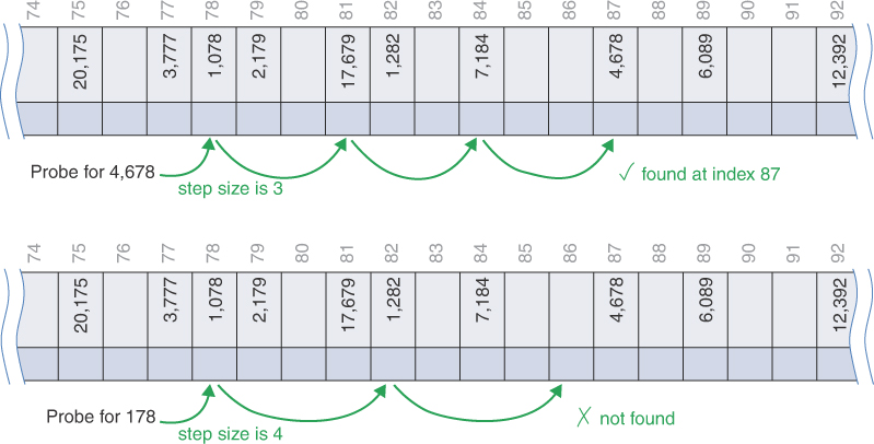
FIGURE 11-16 Double hashing
Implementing double hashing is only slightly more complicated than linear or quadratic probing. You still need a generator that loops over the possible indices, but this time you need to apply the secondary hash function to get the step size. That step should be less than or equal to a prime number below the size of the array. Listing 11-10 shows an implementation for that generator.
The doubleHashProbe() generator starts by immediately yielding the first cell index folded over the possible range of cells. This is a little different from the approach in the linear and quadratic probes. The reason: you don’t have to determine the step size if the first cell ends up being the desired one. Like the other probes, it doesn’t need to know whether the caller seeks an empty or filled cell. If the caller finds an acceptable cell, it will exit its loop through the generator sequence, skipping the calculation of the step size. If the loop continues, then the generator calls doubleHashStep() to compute the step size. That value is used in a loop similar to those of the linear and quadratic probes. The difference is that it starts with 1 times the step size added to the start index and continues through all possible cells.
The doubleHashStep() function computes the step size for the given key. First, it gets the largest prime number that is smaller than the array size by calling primeBelow(). Next, it reapplies the hash function, simpleHash(), to the key (although it would be better to use a different hash function here). The large integer it produces gets mapped to the range of the smaller prime number using the modulo operator. The remainder is subtracted from the prime so that the step size falls in the range [1, prime].
LISTING 11-10 The doubleHashProbe() Generator for Open Addressing
def doubleHashProbe(                  # Generator to determine probe interval
      start, key, size):              # from a secondary hash of the key
   yield start % size                 # Yield the first cell index
   step = doubleHashStep(key, size)   # Get the step size for this key
   for i in range(1, size):           # Loop over all remaining cells using
      yield (start + i * step) % size # step from second hash of key

def doubleHashStep(key, size):        # Determine step size for a given key
   prime = primeBelow(size)           # Find largest prime below array size
   return prime - (                # Step size is based on second hash and
      simpleHash(key) % prime)     # is in range [1, prime]

def primeBelow(n):                 # Find the largest prime below n
   n -= 1 if n % 2 == 0 else 2     # Start with an odd number below n
   while (3 < n and not is_prime(n)): # While n is bigger than 3 or
      n -= 2                       # is not prime, go to next odd number
   return n                        # Return prime number or 3
The primeBelow() function is a straightforward math calculation. It starts by finding an odd number below the parameter, n, by subtracting either 1 or 2 from it, depending on whether n is even or odd. The while loop decrements n by 2 until it either finds a prime or reaches 3.
To save some time, the primeBelow result could be stored in the HashTable object and recomputed only when the array size changes. The step size changes based on the key, so it cannot be stored as efficiently. You would essentially need a hash table to look up the step size for each key!
Using Double Hashing in the Open Addressing Visualization Tool
As with the other methods, you can set the probe type whenever the hash table is empty in the HashTableOpenAddressing Visualization tool. To see a good example of the probes at work, you need to fill the table rather full, say to about nine-tenths capacity or more. Try creating a hash table of 41 cells with the maximum load factor of 0.9. Set the probe type by selecting the Use doubleHashProbe button. Fill most of the table with 30 random keys (perhaps without animating the hashing to go faster).
With such high load factors, only about a quarter of new, random data items will be inserted at the cell specified by the first hash function; most will require extended probe sequences. Try inserting one or two more random keys by using the Random Fill button with animation of the hashing.
Try finding some existing keys in the crowded table. When a search needs a multistep probe sequence, you’ll see how all the steps are the same size for a given key, but that the step size is different. Some step sizes can be large and, when wrapping around the table size, can take what looks like a random path among the cells.
The Visualization tool does not show the code for calculating the step size. In fact, the code is not shown for any of the probe sequence generators. You can still see the patterns they produce, however, by following the arrows indicating the cells being probed. The next section discusses the step-by-step execution of double hashing probes.
Double Hashing Example
The double hashing algorithm has many steps. If you haven’t looked at the Visualization tool, here’s an example of how a series of insertions works. We start with an empty HashTable created with the doubleHashProbe() as its probe sequence (see Listing 11-10). We create the hash table with an initial size of 7 (which is different than the Visualization tool default size of 2). As we insert keys, the hash function computes where to store them and how big the steps should be to probe for open addresses. When the load factor gets too large, the table grows to accommodate more key-value pairs.
Table 11-2 shows how each insertion probes to find the cell to modify. The first key inserted is 1. The simpleHash() function just returns the same integer. That makes it easy to see how insertion works (but it’s a terrible hash function in general). Using the same integer also clarifies what the step size will be for double hashing. The first prime below 7 is 5. Subtracting 1 mod 5 from 5 leaves 4 as the step size. Because cell 1 is empty, however, the step size doesn’t matter, and item 1 is inserted into cell 1.
Table 11.2 Filling a Hash Table Using Double Hashing
Item Number | Key |
| Step Size | Total Cells | Prime Below | Probe Sequence After |
|---|---|---|---|---|---|---|
1 | 1 | 1 | 4 | 7 | 5 | |
2 | 38 | 3 | 2 | 7 | 5 | |
3 | 37 | 2 | 3 | 7 | 5 | |
4 | 16 | 2 | 4 | 7 | 5 | 6 |
5 | 20 | 3 | 6 | 17 | 13 | 9 |
6 | 3 | 3 | 10 | 17 | 13 | 13 |
7 | 11 | 11 | 2 | 17 | 13 | |
8 | 24 | 7 | 2 | 17 | 13 | |
9 | 4 | 4 | 9 | 17 | 13 | 13, 5 |
10 | 16* | 16 | 15 | 37 | 31 | |
11 | 10 | 10 | 21 | 37 | 31 | |
12 | 31 | 31 | 31 | 37 | 31 | |
13 | 18 | 18 | 13 | 37 | 31 | |
14 | 12 | 12 | 19 | 37 | 31 | |
15 | 30 | 30 | 1 | 37 | 31 | |
16 | 1* | 1 | 30 | 37 | 31 | |
17 | 19 | 19 | 12 | 37 | 31 | |
18 | 85 | 11 | 8 | 37 | 31 | 19, 27 |
The second key inserted, 38, follows the same pattern. After hashing and taking the modulo with 7, the probe starts at index 3. It would get a different step size of 2 based on 5 – (38 mod 5), but again, that doesn’t matter because cell 3 is empty. The third key inserted, 37, maps to index 2, which is also empty.
On the fourth key, 16, we hit the first collision. The simpleHash() maps it to index 2, which holds key 37. The step size for that key is 5 – (16 mod 5) = 4. The second probe goes to cell 6 (2 + 4), which is empty, so key 16 gets stored there. The table shows cell 6 in the Probe Sequence After simpleHash column.
At this point, four items are stored in the hash table. The table has seven cells, so the load factor is now 4/7, which is larger than the default maxLoadFactor of 0.5. The insert() method calls the __growTable() method after the fourth item is inserted. The table grows to hold 17 cells, and the four items are rehashed into them as follows:
0 | 1 | 2 | 3 | 4 | 5 | 6 | 7 | 8 | 9 | 10 | 11 | 12 | 13 | 14 | 15 | 16 |
1 | 37 | 38 | 16 |
All of the keys rehash into cells of the expanded table at their initial hash addresses based on the new size.
The fifth item to insert has key 20. That hashes to cell 3 in the 17-cell table, which is occupied. The step size is 6, which is calculated using the largest prime below the table size, which is 13 (step = 13 – (20 mod 13)). Probing six cells away finds cell nine to be empty, so that’s where item 20 lands.
The sixth item to insert has key 3. That also hashes to the occupied cell 3. The secondary hashing leads to a step size of 10, and the next probe finds cell 13 to be empty. Item 3 gets placed in cell 13, avoiding the enlargement of any of the clusters. These last insertions of keys 20 and 3 illustrate how two keys, whose primary hash addresses collide, avoid creating clusters by using different step sizes after the initial probe.
The seventh item with key 11 finds cell 11 empty and lands there. That pattern repeats for item 8, key 24, which is stored in the empty cell 7.
More collisions occur with the ninth item, which has a key of 4. The contents of the array just before the insertion of that item are
0 | 1 | 2 | 3 | 4 | 5 | 6 | 7 | 8 | 9 | 10 | 11 | 12 | 13 | 14 | 15 | 16 |
1 | 37 | 38 | 24 | 20 | 11 | 3 | 16 |
Cell 4 is occupied, so it computes the step size of 9 (13 – (4 mod 13)). The next cell checked is 13. That cell is full, too, so it probes at 5 (13 + 9 % 17 = 5), which is empty. Key 4 is stored there, forming a cluster of three filled cells.
Storing the ninth item in a table of 17 cells brings the load factor to 9/17, which exceeds 0.5. The table grows again to hold 37 cells, and the nine items are reinserted into it. One collision occurs during the reinsertions (key 38 would normally go at index 1 in a 37-cell table but gets stored at cell 25 (1 + (31 – (38 mod 31))).
As Table 11-2 shows, items 10 through 17 are inserted without any collisions. That behavior is typical when the load factor is reduced after growing the table. Looking at the details, you can see that item 10 is actually a duplicate key to item 4, as indicated by the asterisk (*). Both have a key of 16, so the second insertion becomes an update to the value associated with that key. Item 16 is another duplicate; this time it’s key 1. It also immediately finds the key at cell 1 and doesn’t need to probe other cells before updating the value.
The eighteenth item produces a collision. It’s a new key, 85, which hashes to cell 11 (because the table is now of length 37). Because key 11 is stored in cell 11, the double hashing determines that it should step by eight cells. Probing cell 19 finds it occupied with key 19 from the previous insertion, so it moves on to store that key in the available cell 27.
As you can see from this example, collisions do cause some items to be placed in cells different than their original hash location. The chance of a collision increases as the load factor goes up. The 18 insertions filled 16 cells of the table because two of the keys were duplicates of previous keys. That puts the table load factor at 16/37. After inserting three new keys, the table must grow again, keeping the chance of collision low and the number of clusters small.
Table Size a Prime Number
Double hashing requires the size of the hash table to be a prime number. To see why, imagine a situation in which the table size is not a prime number. For example, suppose the array size is 15 (indices from 0 to 14), and that a particular key hashes to an initial index of 0 and a step size of 5. The probe sequence would be 0, 5, 10, 0, 5, 10, and so on, repeating endlessly. Only these three cells would ever be examined, so the algorithm will never find the empty cells that might be waiting at 1, 2, 3, and so on. The reduced coverage of the available cells means the algorithm will exhaust all its probes before quitting. In other words, it will crash and burn.
If the array size were instead 13, which is prime, the probe sequence would eventually visit every cell. It would be 0, 5, 10, 2, 7, 12, 4, 9, 1, 6, 11, 3, and so on. If there were even one empty cell, the probe would find it. Using a prime number as the array size makes it impossible for any number to divide it evenly (other than 1 and the prime itself), so the probe sequence will eventually check every cell.
Despite the added time needed to find prime numbers, double hashing wins overall when choosing the best probe sequence for open addressing.
Separate Chaining
In open addressing, collisions are resolved by looking for an open cell in the hash table. A different approach is to install a linked list or binary tree at each index in the hash table. A data item’s key is hashed to the index in the usual way, and the item is inserted into the structure at that index. Other items that hash to the same index are simply added to the structure; there’s no need to search for empty cells in the primary array. Figure 11-17 shows how separate chaining looks. The top version shows sorted linked lists in the table cells, and the bottom shows balanced, binary trees.

FIGURE 11-17 Examples of separate chaining
Separate chaining is conceptually somewhat simpler than the various probe schemes used in open addressing. The code, however, is longer because it must include the mechanism for the linked list or trees, usually in the form of an additional class.
The HashTableChaining Visualization Tool
To see how separate chaining works, start the HashTableChaining Visualization tool. It displays an empty array, as shown in Figure 11-18. Like the open addressing tool, it starts with two empty cells that will grow as new items are added. The linked lists start from these cells and grow downward.

FIGURE 11-18 Separate chaining in the HashTableChaining Visualization tool
The buttons in the HashTableChaining Visualization tool are nearly identical to those of the HashTableOpenAddressing tool, except that the probe choice buttons have been removed. Despite the similar appearance, the operations have quite a few differences.
Try inserting some items. As with the open addressing tool, the keys can be strings or integers, and the same simpleHash() function determines which cell of the array should contain the key. The hashing box, item count, and load factor limit are at the top to keep them out of the way as the linked lists grow downward.
The linked lists are unsorted (we discuss the option of keeping them sorted shortly). New items are appended to the end of the list. After the total number of items in all the lists divided by the number of cells exceeds the maxLoadFactor limit, a similar __growTable() function creates an array that’s at least twice as big with a prime number of cells. The items are rehashed to find their location in the new array.
It might seem strange that the separate chaining tool starts with a maxLoadFactor of 1.0 (100%). You saw how congested hash tables caused problems in open addressing. Congestion can be a problem in separate chaining, too, but in a different way.
Try filling the array with 30 random keys (you can turn off the animation of the insertion by deselecting the Animate Hashing option before filling). You will likely get a table that looks similar to the one in Figure 11-19. Most (14) of the linked lists have one item, a few (5) have two items, and two have three items in the example (the lists in cells 26 and 43). The 30 items are stored in 21 cells of the 47-cell table. That’s typical of separate chaining; the items are spread out over many, but not all, of the cells and the length of the chains is relatively short.
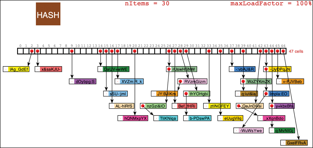
FIGURE 11-19 A separate chaining hash table with 30 random items
With items in the hash table, try a few searches. If you click the index number for a cell, it will enter that number in the text entry box. You can use that index as a search key. If you click index 26 of the hash table in Figure 11-19, enable the Animate Hashing option, and then select Search, you can see how the hashing finds cell 26 immediately and must step through each of the three items in the linked list to determine that no item with key 26 is in the hash table. Searches for existing keys also may step through a few items before finding the goal key.
Try deleting a few items (remembering that you can click a key to copy it to the text entry box). The search mechanism for the item to delete is the same, and the animation shows the steps it takes. Unlike open addressing, the item is deleted from the linked list, not replaced with a special deleted value.
In the Visualization tool, the items are placed roughly below the hash table cell in which they belong but are adjusted in position to avoid obscuring other items and to reduce some of the overlapping arrows. The arrows have different lengths, making the number of links in each list harder to see. For example, cell 16 in Figure 11-19 holds a linked list of one item, “AL-hlRfS,” and that item was placed below all the others due to the presence of other items inserted before it.
Load Factors
The load factor is typically managed differently in separate chaining than in open addressing. In separate chaining it’s normal to put N or more items into an N cell array; thus, the load factor can be 1 or greater. There’s no problem with this; some locations simply contain two or more items in their lists.
Of course, if the lists have many items, access time takes longer because access to a specified item requires searching through an average of half the items on the list. Finding the initial cell is fast, taking O(1) time, but searching through a list takes time proportional to M, the average number of items on the list. This is O(M) time. Thus, you don’t want the lists to become too full. If you use binary trees, the search time is O(log M). You can let the trees grow more than lists do, if they remain balanced.
A load factor of 1, as shown in the initial Visualization tool, is common. In open addressing, performance degrades badly as the load factor increases above one-half or two-thirds. In separate chaining the load factor can rise above 1 without hurting performance very much. This insensitivity to the load makes separate chaining a more robust mechanism and reduces unused memory, especially when it’s hard to predict in advance how much data will be placed in the hash table. There is still a need to grow the hash table when the load factor (or the longest list or deepest tree) grows too big, but the decision metric is different.
You can experiment with load factor limits from 0.5 to almost 2.0 by creating new tables with the New button in the Visualization tool. You can also fill with up to 99 randomly keyed items, and the growth of the hash table size is limited to 61 cells. This limitation creates some very congested separate chaining hash tables. The scroll bars will be adjusted to allow you to view the whole structure. The visualization slows down for large tables as it attempts to adjust the links to avoid overlaps.
Duplicates
Duplicate keys could be allowed in separate chaining but typically are not for all the same reasons applied to open addressing, plus the reasons mentioned for linked lists and binary trees. If they are allowed, all items with the same key will be inserted in the same list or tree. Therefore, if you need to discover all of them, you must search more of the list or tree in both successful and unsuccessful searches. Deletion must also search further when deleting all items with the same key. These extended searches lower performance.
Deletion
In separate chaining, deletion is easier than in open addressing. There’s no need for a marker for a deleted item. The algorithm hashes to the proper table cell and then deletes the item from the list or tree. If the item is the last item stored in that cell, the cell can be set back to empty, if minimum memory usage is important. Leaving an empty tree or list header in the cell does not harm garbage collection.
Table Size
With separate chaining, making the table size a prime number is not as important as it is with open addressing. There are no probe sequences in separate chaining, so you don’t need to worry that a probe will go into an endless sequence or not cover all the cells because the step size divides evenly into the array size.
On the other hand, certain kinds of key distributions can cause data to cluster when the array size is not a prime number. We have more to say about this problem when we discuss hash functions.
Buckets
Another approach similar to separate chaining is to use an array at each cell in the hash table instead of a linked list. Such fixed-size arrays are sometimes called buckets (although some hash table descriptions use the term “bucket” to mean what we’ve been describing as a “cell” of the hash table). This approach is not as efficient as the linked list approach, however, because of the problem of choosing the size of the buckets. If they’re too small, they may overflow, requiring growth of the hash table and rehashing all the items. If the buckets are too large, they waste memory. Linked lists and binary trees, which allocate memory dynamically, don’t have this problem.
Python Code for Separate Chaining
There are many commonalities between the code for open addressing and separate chaining. Listing 11-11 shows the core class definition for a separate chaining HashTable. Compare that with the definition shown in Listing 11-2 for open addressing. There are three differences: there’s an import statement to get the KeyValueList class, there’s no probe parameter in the constructor because there is no probe sequence, and the default value for maxLoadFactor is higher. This class uses a slightly revised version of the LinkedList class from Chapter 5, “Linked Lists,” for the separate chaining. You could also use the AVLTree from Chapter 10, “AVL and Red-Black Trees.” It only needs to support the same interface of creation, insertion, search, deletion, and traversal. We discuss the KeyValueList class and the tree alternative later.
The constructor for the class could initialize all the cells of the hash table to be empty linked lists. Doing so, however, would increase the memory consumed by the structure and add time to the construction process. It’s preferable to wait until items need to be inserted in cells before creating the chain (list or tree) to hold them. Note that the utility methods __len__(), cells(), and hash() remain identical. Now let’s look at what changes for separate chaining.
Perhaps the most significant change is the lack of a __find() method. For other data structures you used a find method to locate where an item is stored. In the case of separate chaining, you can use the hash function to find the cell (or bucket), and the chain’s search and find methods to locate the item within that cell.
LISTING 11-11 The Core HashTable Class for Separate Chaining
from KeyValueList import *

class HashTable(object):           # A hash table using separate chaining
   def __init__(                   # The constructor takes the initial
         self, size=7,             # size of the table,
         hash=simpleHash,          # a hashing function, and
         maxLoadFactor=1.0):       # the max load factor before growing
      self.__table = [None] * size # Allocate empty hash table
      self.__nItems = 0            # Track the count of items in the table
      self.__hash = hash           # Store given hash function, and max
      self.__maxLoadFactor = maxLoadFactor # load factor

   def __len__(self):              # The length of the hash table is the
      return self.__nItems         # number of cells that have items

   def cells(self):                # Get the size of the hash table in
      return len(self.__table)     # terms of the number of cells

   def hash(self, key):            # Use the hashing function to get the
      return self.__hash(key) % self.cells() # default cell index
The search() method for the separate chaining HashTable simply hashes the key to a cell index, i; checks whether cell i has been filled with a list object; returns None if it doesn’t or the result of searching for the key in the list. Listing 11-12 shows the implementation. All the complexity of the probe sequence has gone away and is replaced by the, hopefully well-understood, operation of the chain structure (linked list or tree).
The insert() method is also simplified. After hashing the key to get the cell index, i, it checks whether the cell is filled with a list object. If not, a new, empty key-value list is created and stored there. The main work of the insertion happens using the KeyValueList’s insert() method, shown later. Like the tree implementations, the insert method returns a flag indicating whether a new node was created (as opposed to updating an existing key’s value). When a new node is created, it increments the number of items and checks the load factor. If it has crossed the threshold, the hash table must be enlarged. It is important to count the number of items in all the lists stored in hash table cells, not the number of lists, as we discuss shortly. After managing the growth of the table, insert() can return the flag indicating whether a new node was added to the hash table.
The __growTable() method starts off the same as for open addressing. It keeps a local variable pointing at the old table while it allocates a new one with a size that’s a prime number at least twice the size of the previous one. Then it rehashes each of the items in the old table into the new one. The traversal of the old table is a loop through all its cells. Filled cells must be traversed using the chain’s traverse() method. The key-value tuples are stored in the item variable and then passed as the two arguments to the hash table’s own insert() method.
LISTING 11-12 The Search and Insert Methods for a Separate Chaining HashTable
class HashTable(object):           # A hash table using separate chaining
…
   def search(self,                # Get the value associated with a key
              key):                # in the hash table, if any
      i = self.hash(key)           # Get cell index by hashing key
      return (None if self.__table[i] is None else # If list exists,
              self.__table[i].search(key)) # search it, else None

   def insert(self,                # Insert or update the value associated
              key, value):         # with a given key
      i = self.hash(key)           # Get cell index by hashing key
      if self.__table[i] is None:  # If the cell is empty,
         self.__table[i] = KeyValueList() # Create empty linked list
      flag = self.__table[i].insert(key, value) # Insert item in list
      if flag:                     # If a node was added,
         self.__nItems += 1        # increment item count
         if self.loadFactor() > self.__maxLoadFactor: # When load
            self.__growTable()     # factor exceeds limit, grow table
      return flag                  # Return flag to indicate update

   def __growTable(self):          # Grow the table to accommodate more items
      oldTable = self.__table      # Save old table
      size = len(oldTable) * 2 + 1 # Make new table at least 2 times
      while not is_prime(size):    # bigger and a prime number of cells
         size += 2                 # Only consider odd sizes
      self.__table = [None] * size # Allocate new table
      self.__nItems = 0            # Note that it is empty
      for i in range(len(oldTable)): # Loop through old cells and
         if oldTable[i]:           # if they contain a list, loop over
            for item in oldTable[i].traverse(): # all items
               self.insert(*item)  # Re-hash the (key, value) tuple
Let’s look at the implementation of the KeyValueList class. It’s a specialized version of the LinkedList class from Chapter 5 where every link item holds a (key, value) tuple, as shown in Listing 11-13. The definition starts off by importing the LinkedList class and defining some accessor functions for getting keys and values from the links.
The insert() method differs from its parent class in the way it handles insertion of duplicate keys. The simple LinkedList version always inserts new items at the beginning of the list. The KeyValueList must update an existing value if the key is already in the list. It first finds any link with a matching key (using the parent class’s find() method with the itemKey function to extract the key from each link’s tuple). If no such link is found, it uses the parent class’s insert() method to put the (key, value) tuple at the start of the list. It returns True to indicate the addition of a new item. If a link with a matching key is found, it updates the data for that link with the (key, value) tuple and returns False to indicate no additions were made.
LISTING 11-13 The Definition of the KeyValueList Class
import LinkedList

def itemKey(item): return item[0]  # Key is first element of item
def itemValue(item): return item[1] # Value is second element of item

class KeyValueList(LinkedList.LinkedList): # Customize LinkedList

   def insert(self, key, value):   # Insert a key + value in list
      link = self.find(key, itemKey) # Find matching Link object
      if link is None:             # If not found,
         super().insert((key, value)) # insert item at front
         return True               # return success
      link.setData((key, value))   # Otherwise, update existing link's
      return False                 # datum and return no-insert flag

   def search(self, key):          # Search by matching item key
      item = super().search(key, key=itemKey) # Locate key + value
      return itemValue(item) if item else None # Return value if any

   def delete(self, key):          # Delete a key from the list
      try:                         # Try the LinkedList deletion by key
         item = super().delete(key, itemKey)
         return item               # If no exceptions, return deleted item
      except:                      # All exceptions mean key was not
         return False              # found, so return False

   def traverse(self):             # Linked list traverse generator
      link = self.getFirst()       # Start with first link
      while link is not None:      # Keep going until no more links
         yield link.getData()      # Yield the item
         link = link.getNext()     # Move on to next link
The search() method uses the parent class’s search() method to get the first link with a matching key, if any. It returns the associated value if a link is found and None otherwise.
The delete() method differs the most from its parent. In the simple LinkedList version, delete() throws an error if the list is empty or the key is not found. The KeyValueList uses a try except clause to get the result from the parent delete() method. If an item is found and deleted, it returns that item. If an error occurs, it returns False to indicate the key was not found.
Finally, the traverse() method of KeyValueList is nearly the same code as its parent class but uses a yield statement to make it a generator that yields the (key, value) tuples in the list.
Returning to the separate chaining HashTable implementation, you can define its traverse() method, as shown in Listing 11-14, to use that of the KeyValueList. The loops are similar to those used in __growTable(). The differences are that the traverse() method loops over the current hash table cells instead of the old copy, and it yields the items it finds instead of reinserting them.
LISTING 11-14 The traverse() and delete() Methods for Separate Chaining
class HashTable(object):                 # A hash table using separate chaining
…
   def traverse(self):                   # Traverse the key, value pairs in table
      for i in range(len(self.__table)): # Loop through all cells
         if self.__table[i]:             # For those cells containing trees,
            for item in self.__table[i].traverse(): # traverse
               yield item                # the tree in-order yielding items

   def delete(self,                      # Delete an item identified by its key
              key,                       # from the hash table. Raise an exception
              ignoreMissing=False):      # if not ignoring missing keys
      i = self.hash(key)                 # Get cell index by hashing key
      if self.__table[i] is not None:    # If cell i is not empty, try
         if self.__table[i].delete(key): # deleting item in tree and
            self.__nItems -= 1           # if found, reduce count of items
            return True                  # Return flag showing item was deleted
      if ignoreMissing:                  # Otherwise, no deletion. If we ignore
         return False                    # missing items, return flag
      raise Exception(                   # Otherwise raise an exception
         'Cannot delete key {} not found in hash table'.format(key))
Before we discuss the delete() method, let’s look at the order in which hash table items will be traversed.
Traversal Order in Hash Tables
What order should a hash table traverse its items? In binary search trees, you have the option to traverse in-order, pre-order, or post-order. Is there a way to do the same in hash tables? The orderings in trees are based on the structure of the tree with parent, left child, and right child nodes. There is no equivalent structure over all the items in the hash table (even though there can be such a structure in a single cell with separate chaining).
The order that the traverse() methods shown in Listing 11-14 and Listing 11-8 would yield items is based primarily on their hash address. That’s a combination of both the hash function and the size of the hash table. If you wanted the keys to be yielded in ascending order, you would need to either reverse the hash function or collect all the keys and sort them. Reversing a hash function is very hard to do in most cases. Sorting the keys, as you’ve seen, could take O(N×log N) time. In general, hash tables return the keys in “arbitrary” (unpredictable) order. If the caller needs them in order, it can sort them (by key or value). Interestingly, Python’s dict hash table returned keys in arbitrary order in early versions. In version 3.7 and beyond, it returns them in insertion order.
Note that in separate chaining, the items within each cell are traversed according to the traversal order of the list or tree that is used. In the KeyValueList implementation, the list keeps the items in reverse insertion order. When the hash table grows, however, the rehashing of the items goes through the linked lists and reverses the previous insertion order. That makes the ultimate traversal order very hard to predict. If you use an AVL tree for chaining, then the items in each tree could be traversed in key order, but due to rehashing, they still will be yielded by the hash table’s traversal in arbitrary order.
The delete() Method for Separate Chaining
The last method of the separately chained hash table implementation shown in Listing 11-14 is delete(). Like insert(), the code for delete() is simpler than what was needed for open addressing. This method computes the hash address of the key and then uses the KeyValueList delete() method to remove the item, if the list is present. If that list reports that an item was deleted, it reduces the item count for the hash table and returns True to signal the deletion of the item. If minimal memory usage is important, the cell should be set to None before returning True when the deletion results in an empty list or tree.
If the cell is empty or the tree doesn’t find the key to delete, the ignoreMissing parameter determines whether to return False or raise an exception.
Which Type of Chaining Should You Use?
Separate chaining can use a number of secondary structures to store the items in each cell. Lists and trees are very common, and sometimes small arrays (when dynamic allocation of new storage is being avoided). There is no single type that’s best for all use cases. Some structures are more efficient than others depending on the hash function and the keys inserted.
The most important factors are the maximum number of items in a cell and the number of times they will be searched. If the hash function is very good, it will distribute the keys evenly among all the table cells. If N items are stored in M table cells, the average number of items per cell is N/M. Note that this is exactly the same as the load factor for the hash table. In the separate chaining implementation, we used a maxLoadFactor of 1.0 as the default value. With a good hashing function, the average number of items stored in a cell should be 1, at most. There will be some cells with two items, some with none, and very few with three or more items.
If no cell contains more than three items, it makes sense to use the simplest of structures for separate chaining, the linked list. The items don’t need to be kept sorted because you only need to compare at most three keys. Inserting into an unsorted list is normally an O(1) operation. In the case of separate chaining, however, you must search the entire list to see if it is a duplicate key. Searching that list takes O(N)—or O(N/M) in this case—for the expected average length of the list. Maintaining the load factor, N/M, at 1.0 or below means that searching the unsorted list and inserting are both expected to be O(1).
Sorted lists don’t speed up a successful search, but they do cut the time of an unsuccessful search in half. As soon as an item larger than the search key is reached, which on average is half the items in a list, the search can be declared a failure. That would become important the longer the lists grow. Deletion times are also cut in half in sorted lists.
If many unsuccessful searches are anticipated, it may be worthwhile to use the slightly more complicated sorted list rather than an unsorted list. An unsorted list, however, wins when insertion speed is more important. An example of that might be the use of a hash table to store all the entries for a “pick 6” lottery. Each lottery participant picks a sequence of six numbers. The hash table is used to store each participant’s contact info, so the key is the sequence of numbers, and the data is a list of people who picked that sequence. There could be millions of these sequences, but because there will be only one search for the winning sequence chosen by the lottery managers, there will be very few searches of the hash table (both successful and unsuccessful). There’s little point to spending time during the insertion to sort the keys.
The choice of the secondary structure to use in separate chaining can be affected by the choice of hash function too. Although there are many good hash functions, there are also some bad ones. If a particular application either chooses a bad hash function or somehow runs across a group of keys that hash to just one or two addresses in the hash table using that function, the number of items in one cell can grow as large as N. In that unlikely case, a balanced binary tree like the AVL tree could be best. That makes the insert and search operations within each cell O(log N) instead of O(N). This is a degenerate case where the hash function doesn’t spread the data over a broad number of cells, so the more efficient tree structures are an improvement over lists.
We return to the question of when to use separate chaining versus open addressing when we discuss hash table efficiency later in this chapter.
Hash Functions
In this section we explore the issue of what makes a good hash function and see how we can improve the approach to hashing strings mentioned at the beginning of this chapter.
Quick Computation
A good hash function is simple, so it can be computed quickly. The major advantage of hash tables is their speed. If computing the hash function is slow, this speed will be degraded. A hash function with many iterations or levels of computation is not a good idea. Many are based on sophisticated math. If they involve a lot of multiplications and divisions, especially on a computing platform without hardware support for those kinds of operations, they could take quite a bit of time.
The purpose of a hash function is to take a range of key values and transform them into index values in such a way that the hash addresses are distributed randomly across all the indices of the hash table. Keys may be completely random or not so random.
Random Keys
A so-called perfect hash function maps every key into a different table location. This is rarely possible in practice. A special case happens when the keys are unusually well behaved and fall in a range small enough to be used directly as array indices. For example, a manufacturer gives numbers for each of the parts it creates. The numbers started at 1,000 and go up to the number of things they have ever produced, say 10,000 over the past 50 years. Because they were created to be unique and with no gaps, these could easily be used directly as array indices without hashing, by simply having a hash function that subtracts 1,000 from the part number. These are unusually well-behaved keys.
If you need to store only a few of these part numbers, say the hundred parts currently kept in inventory, then it’s possible to create a perfect hashing function that maps them to unique indices in a smaller array. The perfect hashing function needs to map each of the hundred part numbers to a unique index. You saw the Huffman coding algorithm in Chapter 8, “Binary Trees,” which came up with a unique bit sequence for every letter used in a message. Similar techniques can be used to assign a unique index to every part number.
In most applications, however, it’s impossible to forecast what keys will be inserted in the hash table. Without knowing the number and type of keys, it’s impossible to build a perfect hashing function. So typically, you make assumptions. In this chapter we’ve assumed that the transformed keys were randomly distributed over a large numeric range. In this situation the hash function
index = key % arraySize
is satisfactory. It involves only one more mathematical operation, and if the keys are truly random, the resulting indices will be random too, and therefore well distributed. If the keys share some common divisor(s), you can reduce the chance that they cause collisions by choosing arraySize to be a prime number (and hoping that prime number is not the common divisor).
Nonrandom Keys
Data is often distributed nonrandomly. In fact, it’s very rare to find truly randomly (mathematicians would call it uniformly) distributed data.
Let’s consider some examples for keys: a timestamp key such as the milliseconds that have elapsed since a particular point in time and an IP address on the Internet. Typically, these kinds of keys are not uniformly distributed across all the possible values; they concentrate in ranges. The millisecond timestamps may be for events over a short duration, such as log messages on a computer server over the past week, or perhaps for some past events, such as the births of a group of people. Those births are all likely to be concentrated on dates in the past century, not uniformly spread out over tens of thousands of years. Even within the past century, the birth rate rises and falls, leaving an uneven distribution. For the IP addresses, it’s rare to get a set of data that samples the addresses from all over the world. Typically, there will be many references to local IP addresses and smaller numbers sprinkled from whatever regions communicated with the computer or network appliance that collects the data.
Many keys that might be used have an internal structure. IP addresses are 32-bit or 128-bit numbers organized into four octets or eight 16-bit words. Various blocks of addresses are reserved for different purposes. Any particular set of keys is likely to have many of its keys from a few blocks, and none from most of them.
Part numbers for manufacturers typically have structure too. Let’s look at an example of a system that uses car part numbers as keys and discuss how they can be hashed effectively. Perhaps these part numbers are of the form
033-400-03-94-05-0-535
This number, 033-400-03-94-05-0-535, might be interpreted as follows:
Digits 0–2: Supplier number (1 to 999, currently up to 70)
Digits 3–5: Category code (100, 150, 200, 250, up to 850)
Digits 6–7: Month of introduction (1 to 12)
Digits 8–9: Year of introduction (00 to 99)
Digits 10–11: Serial number (1 to 99, but never exceeds 100)
Digit 12: Toxic risk flag (0 or 1)
Digits 13–15: Checksum (sum of other fields, modulo 1000)
If you ignore the separating hyphens, the decimal key used for the preceding 16-digit part number would be 0,334,000,394,050,535. The keys for the parts are not randomly distributed over all possible numbers. The majority of numbers from 0 to 9,999,999,999,999,999 can’t actually occur (for example, supplier numbers higher than 70, category codes that aren’t multiples of 50, and months from 13 to 99). Also, the checksum is not independent of the other numbers. Some work should be done to these part numbers to help ensure that they form a range of more truly random numbers.
Don't Use Nondata
The key fields should be squeezed down until every bit counts. For example, the category codes in the car part numbers should be changed to run from 0 to 15 (corresponding to the values 100, 150, …, 850 that appear there). The checksum should be removed from the calculation of the hash because it doesn’t add any additional information; it’s deliberately redundant. Various other bit-twiddling techniques are appropriate for compressing the various fields in the key into the unique values they represent.
The address in memory of the key or the record containing the key should never be used in the hash function. In other words, if the key is accessed through a reference pointer, don’t use the pointer when computing the hash. Use only the part number or other identifying elements referenced by the pointer. The location in memory where the data is stored changes from run to run. Using that location would mean that keys would only match on some runs of the program.
Use All the Data
Every part of the key (except nondata, as just described) should contribute to the hash function. Don’t just use the first four digits, last four digits, or some such abbreviation. The more data that contributes to the key, the more likely it is that the keys will hash evenly into the entire range of indices.
Sometimes the range of keys is so large that it overflows the type of integer values that the programming language supports. Most computing platforms support 32-bit and 64-bit integers. Some embedded processors, however, might support only 16-bit or 8-bit. Regardless of the platform size limit, there will be keys with numeric values that go beyond what can be represented in a single machine word. We show how to handle that overflow when we talk about hashing strings in a moment.
To summarize: The trick is to find a hash function that’s simple and fast, using all the available data, while excluding the nondata and redundant parts of the key.
Use a Prime Number for the Modulo Base
Often the hash function involves creating a number on a large range and using the modulo operator (%) with the table size to map it to the hash address. You’ve already seen that it’s important for the table size to be a prime number when using a quadratic probe or double hashing. If the keys themselves are not randomly distributed, it’s important for the table size to be a prime number no matter what hashing system is used.
To see why a prime number of cells is helpful, consider what happens if many hashed keys are separated in value by some number, X. If X is a divisor of the array size, say ¼ of the size, that large group of keys hash to the same four locations, causing primary clustering. Using a prime table size nearly eliminates this possibility. For example, if the table size were a multiple of 50 in the car part example, the category codes could all hash to index numbers that are multiples of 50 (assuming that code is multiplied into the hash value). With a prime number such as 53, however, you are guaranteed that only keys that hash to multiples of that prime (plus a constant offset) are hashed to the same address. Part numbering and other human-designed schemes rarely use prime numbers like that.
Returning to the example of timestamps as keys, the events represented by timestamps are often periodic. The times can represent things that usually happen at the top of the hour, or every 20 minutes, or every year. The periodic events will create timestamps bunched together around certain peak times. If those peaks are separated by a multiple of the array size, then many keys hash to the same address. Even when they don’t land exactly on multiples of the array size, the bunches can create collisions of hash addresses causing clusters in open addressing or long chains in separate chaining.
The moral is to examine your keys carefully and tailor your hash algorithm to remove any regularities in the distribution of the keys.
Hashing Strings
At the beginning of this chapter, you saw how to convert short strings to key numbers by multiplying digit codes by powers of a constant. In particular, you saw that the three-letter word elf could turn into the number 3,975 by calculating
key = 5*272 + 12*271 + 6*270
This approach has the desirable attribute of involving all the characters in the input string. The calculated key value can then be hashed into an array index in the usual way:
index = key % arraySize
The simpleHash() method shown in Listing 11-3 used a similar calculation but with a base of 256 instead of 27. This calculation allows for many more possible characters in the string (but not all Unicode values).
The simpleHash() method is not as efficient as it might be. When hashing strings, it performs the character conversion, raises 256 to the power i (the position of character in the string), multiplies them, and adds all products in the sum expression:
sum(256 ** i * ord(key[i]) for i in range(len(key)))
This way of expressing the calculation is concise, but it does some extra work that can be avoided. You can eliminate computing the power of 256 by taking advantage of a mathematical identity called Horner’s method. This method states that an expression like
var4*n4 + var3*n3 + var2*n2 + var1*n1 + var0*n0
can be written as
(((var4*n + var3)*n + var2)*n + var1)*n + var0
The base, n, now appears without an exponent, multiplying each parenthesized expression (including var4). To convert this equation into loop form, you start inside the innermost parentheses and work outward. Translating this equation to a Python function results in the following:
def hashString1(key):                    # Use Horner's method to hash a string
   total = 0                             # Sum contribution of all characters
   for i in range(len(key) - 1, -1, -1): # Go in reverse order
      total = total * 256 + ord(key[i])  # Multiply by base, add char i
   return total                          # Return sum
The hashString1() function computes the same hash that simpleHash() does for a string, but with one multiply and one addition per character in the loop. Raising 256 to a power happens by repeating the multiplications.
This approach is a definite improvement because most processors can perform multiplications in a few clock cycles, whereas raising numbers to a power can take much longer. There are two more changes that can help a little more. Multiplying by a power of 2 is the same as shifting the bits of a binary number to the left by that power. In this case, 256 is 28, and you can use the bit shift operator, <<, instead of the multiplication:
def hashString2(key):                    # Use Horner's method to hash a string
   total = 0                             # Sum contribution of all characters
   for i in range(len(key)):             # Go in forward order
      total = (total << 8) + ord(key[i]) # Shift to mult., add char i
   return total                          # Return sum
Bit shifts are supported by every modern processor and are usually faster than multiplication. This example also changes the character index, i, to increase from 0 to the last character of the key. This approach saves a tiny bit of time (a subtraction) and makes the code simpler, although it will produce very different hash values than hashString1() for the same string (other than palindromes). The strings still get hashed to unique values, but the most significant characters—the ones that change the hash value the most—are on the left for the hashString2() function.
The hashString2() function provides a more optimized hash function that will compute a unique number very quickly from every string. There’s another factor to consider, however, and that is the magnitude of the sum. As you shift bits (or multiply), you eventually create numbers bigger than what fits in a machine word. A 64-bit processor could shift the total by 8 bits seven times without overflowing its 64-bit registers. For strings longer than 8 characters (or character points greater than 255), an overflow is likely to occur.
Can we modify the basic approach so we don’t overflow any variables? Notice that the hash address we eventually end up with is always less than the array size because we apply the modulo operator. It’s not the final index that’s too big; it’s the intermediate total values.
With any arithmetic expression using +, *, and –, you can apply the modulo operator (%) at each step in the calculation. Using the operator this way gives the same result as applying the modulo operator once at the end but avoids overflow, at the cost of adding an operation inside the loop. The hashString3() method shows how this looks:
def hashString3(key, size):  # Use Horner's method to hash a string
   total = 0                 # Sum without overflowing
   for i in range(len(key)): # Go in forward order, shift, add char i
      total = ((total << 8) + ord(key[i])) % size # and use modulo
   return total              # Return sum
Most string hashing functions take this approach (or something like it). Various bit-manipulation tricks can be played as well, such as using a size that is a power of 2. That means the modulo operator can be replaced by AND-ing the total with a bit “mask” (for example, total & 0xFFFFFFF). On the other hand, using a power of 2 as the hash table size means that there could be hash table collisions for keys with patterns related to that power of 2, rather than a prime.
You can use similar approaches to convert any kind of string or byte sequence to a number suitable for hashing. Because all data is stored as sequences of bytes, this scheme handles nearly any kind of data.
Folding
Another reasonable hash function involves breaking the key into groups of digits and adding the groups. This approach ensures that all the digits influence the hash value. The number of digits in a group should correspond to the size of the array. That is, for an array of 1,000 items, use groups of three digits each. The folding technique is almost like writing the digit string on a strip of paper, folding the paper between every group of K digits, and then adding the numbers now piled on top of one another.
For example, suppose you want to hash 10-digit telephone numbers for linear probing. If the array size is 1,000, you would divide the 10-digit number into three groups of 3 digits, plus a final digit. If a particular telephone number was 123-456-7890, you would calculate a key value of 123+456+789+0 = 1368. The modulo operator can map those sums to the range of indices, 0–999. In this case, 1368 % 1000 = 368. If the array size is 100, you would need to break the 10-digit key into five 2-digit numbers: 12+34+56+78+90 = 270, and 270 % 100 = 70.
It’s easier to imagine how this operation works when the array size is a multiple of 10. For best results, however, the array size should be a prime number, or perhaps a power of 2, as you’ve seen for other hash functions. We leave an implementation of this scheme as an exercise.
Hashing Efficiency
We’ve noted that insertion and searching in hash tables can approach O(1) time. If no collision occurs, or the separate chains contain one element at most, only a call to the hash function, an array reference, and maybe a link dereference are necessary to find an existing item or insert a new item. This is the minimum access time.
Note that the hash function takes some time to compute, and the amount of time depends on the length of the key and the hashing function. Keys are typically short, perhaps tens of bytes. Because the length of the keys is much shorter than a large N—the number of items stored—you treat the time spent hashing as O(1). When you’re considering hashing a large sequence of bytes—say an entire video file—the time spent hashing could become significant, but it still could be small compared the number of items stored (for example, all the videos available on the Internet).
If collisions occur, access times become dependent on the resulting probe lengths or search of a chain. Each cell accessed during a probe or link in a chain adds another time increment to the search for a vacant cell (for insertion) or for an existing cell. During an access, a cell or link must be checked to see whether it’s empty and whether it contains the desired item.
Thus, an individual search or insertion time is proportional to the length of the probe, length of the chain, or depth of the tree. This variable time must be added to the constant time for the hash function.
The average probe or chain length (and therefore the average access time) is dependent on the load factor (the ratio of items in the table to the size of the table). As the load factor increases, the lengths grow longer.
Let’s look at the relationship between probe lengths and load factors for the various kinds of hash tables we’ve studied.
Open Addressing
The loss of efficiency with high load factors is more serious for the various open addressing schemes than for separate chaining.
In open addressing, unsuccessful searches generally take longer than successful searches. Remember that during a probe sequence, the algorithm stops as soon as it finds the desired item, which is, on average, halfway through the probe sequence. On the other hand, probing must go all the way to the end of the sequence before it’s sure it can’t find an item.
Linear Probing
The following equations show the relationship between probe length (P) and load factor (L) for linear probing. For a successful search, it’s
P = ( 1 + 1 / (1 – L) ) / 2
and for an unsuccessful search, it’s
P = ( 1 + 1 / (1 – L) 2) / 2
These formulas are from Knuth (see Appendix B, “Further Reading”), and their derivation is quite complicated. Figure 11-20 shows the graphs of these equations in the blue (upper) curves. The upper graph shows the probe lengths for successful searches and the lower one shows the lengths for unsuccessful searches.
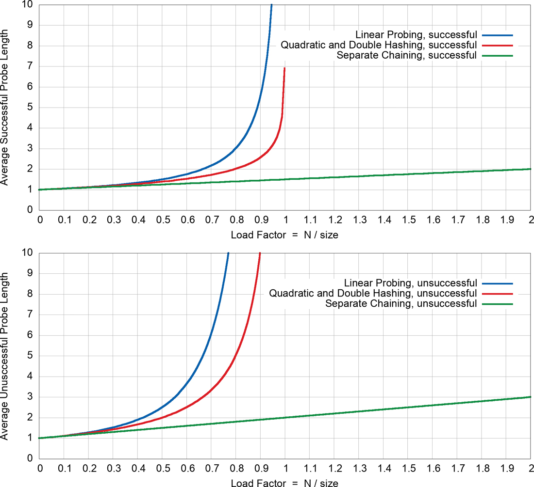
FIGURE 11-20 Successful and unsuccessful probe performance
At a load factor of 0.5, the average successful search takes 1.5 comparisons, and the average unsuccessful search takes 2.5. At a load factor of 2/3, the numbers are 2.0 and 5.0. At higher load factors, the numbers become very large—so high they go off the graph to infinity. We discuss the other lines in the graphs shortly.
The takeaway, as you can see, is that the load factor must be kept under 2/3 and preferably under 1/2. On the other hand, the lower the load factor, the more memory is needed for a given number of items. The optimum load factor in a particular situation depends on the trade-off between memory efficiency, which decreases with lower load factors, and speed, which increases.
Quadratic Probing and Double Hashing
Quadratic probing and double hashing share their performance equations. These equations indicate a modest superiority over linear probing. For a successful search, the formula (again from Knuth) is
P = –ln(1 – L) / L
where ln() is the natural logarithm function. This is like log2(), except the base is the special constant, e ≅ 2.718. For an unsuccessful search, it is
P = 1 / (1 – L)
Figure 11-20 shows the graphs of these formulas using red lines. At a load factor of 0.5, successful searches take about 1.4 probes, whereas unsuccessful ones average 2.0. At a 2/3 load factor, the numbers are about 1.6 and 3.0; and at 0.8, they’re 2.0 and 5.0. Thus, somewhat higher load factors can be tolerated for quadratic probing and double hashing than for linear probing. That shows up in the graph as the red lines lying below the blue lines.
Note that both the red and blue lines climb steeply as the load factor approaches 1.0. That behavior is expected because it means the table is nearly full, and finding a key or an empty slot can take up to N probes.
Separate Chaining
The efficiency analysis for separate chaining is different, and generally easier, than for open addressing.
We want to know how long it takes to search for a key or to insert an item with a new key into a separate-chaining hash table. All of the methods must compute the hash function and determine a starting hash address. The time taken to compute that is a constant, so we focus on the number of key comparisons needed when searching the chain structure. For chaining, we assume that determining when the end of a list or tree has been reached is equivalent to one key comparison. Thus, all operations require 1 + nComps time, where nComps is the number of key comparisons.
Say that the hash table contains size cells, each of which holds a list, and that N data items have been inserted in the table. Then, on average, each list holds N divided by size items:
Average List Length = N / size
This is the same as the definition of the load factor, L:
L = N / size
Therefore, the average list length equals the load factor.
Searching
In a successful search, the algorithm hashes to the appropriate list and then searches along the linked list for the item. On average, half the items must be examined before the correct one is located. Thus, the search time is
P = 1 + L / 2
This is true whether the lists are ordered or not. In an unsuccessful search, if the lists are unordered, all the items must be searched, so the time is
P = 1 + L
These formulas are graphed in Figure 11-20 using the green (lowest) lines. For an ordered list, only half the items must be examined in an unsuccessful search, so the time is the same as for a successful search.
In separate chaining it’s typical to use a load factor of about 1.0 (the number of data items equals the array size). Smaller load factors don’t improve performance significantly, but the time for all operations increases linearly with load factor, so going beyond 2 or so is generally a bad idea. Of course, the open addressing methods must keep the load factor well below 1.0.
Insertion
On the face of it, insertion of a new key is immediate, in the sense that no comparisons are necessary. Because we chose to not allow duplicate keys, however, any existing chain must be searched to determine whether the key is new or a duplicate. That means that insertion behaves exactly like search plus some constant work to either insert the new item at the end (or beginning) of the list or to update the existing data. The hash function must still be computed, and the data inserted or updated, so let’s call the insertion time 1. To stay consistent with the other measures, you can call that a probe length, P, of 1. Finding that the key is new is equivalent to the time taken for an unsuccessful search of an unordered list:
P = 1 + L
If the lists are ordered or the key exists in the chain, then, as with an unsuccessful search, an average of half the items in each list must be examined, so the insertion time is
P = 1 + L / 2
Separate Chaining with Binary Search Trees
If binary search trees are used to organize the items in each cell, there are a few differences from separate chaining with lists. If you want to get the benefit of fast search of the binary tree, it makes the most sense to use one of the self-balancing binary search tree structures (for example, AVL, 2-3-4, or red-black trees). They are more complex to code, but the number of comparisons needed in both successful and unsuccessful searches is proportional to the depth of the tree. The average number of items stored in each tree is the load factor, like it was for lists. That means the average depth of the trees is log2(L). When the load factor is zero, there still is one probe, so the probe lengths are approximately
P = 1 + log2(L + 1)
Inserting into the tree requires finding where the new key belongs, which takes 1 + log2(L + 1) steps. Finding an existing key also takes 1 + log2(L + 1) steps. Searching for a key that is not in the tree stops when there is no child node where the key would normally fit, so it too takes the same number of steps. There are small variations between the exact number of steps in each of these cases.
Compared with the other methods shown in Figure 11-20, the graph for binary search trees would be just below the green line for separate chaining. Both graphs would start at 1.0 and slowly rise as the load factor increases, but the binary search trees would rise more slowly after the load factor becomes greater than 1.0. The difference is so minor for low load factors that the simplicity of chaining with lists outweighs the probe performance. The faster search is a benefit, only if the load factor gets large, or a bad combination of the hash function with the keys being hashed puts large fractions of the N items in a single tree.
Growing Hash Tables
Along with the time spent probing for where to insert a new item, there is also the time spent growing the hash table and rehashing items already stored in it. Both open addressing and separate chaining benefit by keeping the load factor low, so they typically double the hash table size when the load factor exceeds a threshold (that differs for the two types).
How much extra work does reinserting the items cause? Consider the first insertions: when the load factor is low, insertion of a single item happens in O(1) or “constant” time. If you never had to rehash the items, then inserting N of them takes O(N) time. It may not seem intuitive, but allowing hash tables to grow exponentially by doubling in size maintains that O(N) performance.
To see why, let’s assume that you start with a table of size 1 and that you double it every time an insertion makes the load factor exceed 0.5 (we are intentionally setting aside the complexity of choosing prime table sizes here). After the first insertion, the table is doubled to two cells, and the one item is reinserted. The second insertion pushes the load factor over the threshold again, and the two items must be reinserted into the four-cell table. The steps are detailed in Table 11-3.
Table 11.3 Reinsertions When Table Size Doubles
Item | 1 | 2 | 3 | 4 | 5 | 6 | 7 | 8 | 9 | 10 | 11 | 12 | 13 | 14 | 15 | 16 |
Table size | 2 | 4 | 8 | 16 | 16 | 16 | 16 | 32 | 32 | 32 | 32 | 32 | 32 | 32 | 32 | 64 |
Reinsertions | 1 | 2 | 3 | 4 |
|
|
| 8 |
|
|
|
|
|
|
| 16 |
Item | 17 | 18 | 19 | 20 | 21 | 22 | 23 | 24 | 25 | 26 | 27 | 28 | 29 | 30 | 31 | 32 |
Table size | 64 | 64 | 64 | 64 | 64 | 64 | 64 | 64 | 64 | 64 | 64 | 64 | 64 | 64 | 64 | 128 |
Reinsertions |
|
|
|
|
|
|
|
|
|
|
|
|
|
|
| 32 |
At the insertion of the fourth item, the table doubles to hold 16 items, and the 4 items must be reinserted. The fifth item, however, does not cause any doubling or reinsertion. The same conditions hold until you get to the eighth item, when another doubling happens, and the 8 items must be reinserted.
As Table 11-3 shows, the reinsertion work happens every time the number of items reaches another power of 2. There are longer and longer intervals between those expansions. The whole second section of Table 11-3 has no reinsertions until item 32 is inserted. By the time you insert some large number of items, say a million, the number of reinsertions will be
1 + 2 + 3 + 4 + 8 + 16 + … + 262,144 + 524,288
The last number in the sum is the largest power of 2 below one million. Moving out the exception for 3 and writing these as powers of 2 makes the sum:
3 + 20 + 21 + 22 + 23 + 24 + … + 218 + 219
The sum of the powers of 2 should look familiar. It is the same as the count of the nodes in a binary tree going from the root to the leaves. As you saw when analyzing the efficiency of binary trees in Chapter 8, that sum of powers of 2 going from 0 to some level, K, can be written as a formula that depends on a power of 2 itself:
So, the total number of reinsertions is 3 + 2K+1 – 1 or 2 + 2K+1. That looks as though it could become a very large number, which means inserting N items would take a lot more work than O(N). What you have to remember is the relationship between K and N. When you insert a million items, K is 19; and 2K is the largest power of 2 less than or equal to N. In other words, K is the integer just below log2(N). Substituting log2(N) in the equation for the number of reinsertions (and forgetting about getting the integer just below it) leaves
number of reinsertions = 2 + 2log2 (N)+1 = 2 + 2 × 2log2 (N) = 2 + 2 × N = 2(N +1)
That means the number of reinsertions grows linearly as N grows. The original N items were inserted with O(N) work and the reinsertions just increase the constant multiplying N, so the overall complexity is still O(N). Even when you grow the table to be the next prime number larger than twice its current size, the same pattern holds. The number of items to reinsert is always less than half the new table size, and the overall sum of reinserted items does not grow faster than O(N).
Hash Table Memory Efficiency
We’ve noted that hash tables can contain many unused cells under various circumstances. Overall, they still consume O(N) memory to store N items. They need more memory than a simple array because they must store keys along with their associated values (arrays store only the values, and the key is implicit). Keeping the load factor below the thresholds means you need roughly twice as many cells as the number of items, N, but that is still O(N).
We have assumed that the table grows during insertions by doubling its size when needed so that it is never much more than twice N. When you look a bit closer, however, if you first insert P items and then delete some of them to reach N items, open addressing implementations will consume O(P) space. That amount could be significant when P is much larger than N.
For separately chained hash tables, the process of inserting P items and then deleting some to leave N items doesn’t waste quite as much memory as open addressing does because deletions within a chain or tree free up the memory that was being consumed. Only deleting the last item in the chain or tree leaves an empty memory cell or empty chain object.
The other item to note is that traversal time is proportional to the table size. If many items were deleted from a hash table that once held P items, traversal time would still take O(P) to check all the cells. This is the first data structure we’ve seen where traversal could be a bit slower than O(N) where N is the current number of items stored. Deletions in hash tables cause the difference in the time efficiency of traversal. It remains O(N), but N is the maximum number of items inserted, not the current number stored.
Open Addressing Versus Separate Chaining
If open addressing is to be used, double hashing is the preferred system (certainly over quadratic probing). The exception is the situation in which plenty of memory is available and the data won’t expand after the table is created; in this case, linear probing is somewhat simpler to implement and, if load factors below 0.5 are used, causes little performance penalty.
The number of items that will be inserted in a hash table generally isn’t known when the data structure implementation is written, and sometimes not even when the table is created. Thus, in most cases, separate chaining is preferable to open addressing. Allowing the load factor to get large causes major performance penalties in open addressing, but performance degrades only linearly or logarithmically in separate chaining.
When in doubt, use separate chaining. Its drawback is the need for a linked list or binary search tree class, but the payoff is that adding more data than you anticipated won’t cause performance to slow to a crawl.
Hashing and External Storage
At the end of Chapter 9, “2-3-4 Trees and External Storage,” we discussed using B-trees as data structures for external (disk-based) storage. Let’s look briefly at the use of hash tables for external storage.
Recall from Chapter 9 that a disk file is divided into blocks containing many records and that the time to access a block is much longer than any internal processing on data in main memory. For these reasons, the overriding consideration in devising an external storage strategy is minimizing the number of block accesses.
On the other hand, external storage is less expensive per byte, so it may be acceptable to use large amounts of it, more than is strictly required to hold the data, if by so doing you can speed up access time. Hash tables make this speed up possible.
Table of File Pointers
The central feature in external hashing is a hash table containing block numbers, which refer to blocks in external storage. This configuration is similar to the separately chained hash table, but the contents of the table cells point to external blocks rather than a list or a tree in memory. The hash table is sometimes called an index (in the sense of a book’s index). It can be stored in main memory or, if it is too large, stored externally on disk, with only part of it being read into main memory at a time. Even if it fits entirely in main memory, a copy will probably be maintained on the disk and read into memory when the file is opened.
Nonfull Blocks
Let’s assume the same characteristics as the contact database example from Chapter 9 in which the block size is 8,192 bytes, and a record is 1,024 bytes. Thus, a block can hold 8 records. Every entry in the hash table points to one of these blocks. Let’s say there are 100 blocks in a particular file.
The index (hash table) in main memory holds pointers to the file blocks. The hash table has indices from 0 to 99. The contents of cell 11, for example, holds a block number in external storage where a group of records are stored. Those records’ keys hash to 11.
In external hashing it’s important that blocks don’t become full. Thus, you might store an average that’s about half the maximum capacity, so 4 records per block in this example. Some blocks would have more records, and some fewer. There would be about 400 records in the file. This arrangement is shown in Figure 11-21.
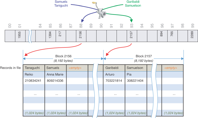
FIGURE 11-21 Hashing to external blocks
All records with keys that hash to the same value are located in the same block. To find a record with a particular key, the search algorithm hashes the key, uses the hash value as an index to the hash table, gets the block number at that index, and reads the block. In the Figure 11-21 example, the name Samuels hashes to address 88 in the 100-block index. That contains block number 2156. Reading that block from disk allows the algorithm to retrieve the full record for Samuels. A similar name like Samuelson could hash to a very different address, 93 in the example, and be stored in another block. Different names like Taniguchi could hash to the same table address, and block, as Samuels. A new key might hash to an empty cell that has no block number.
This process is efficient because only one block access is necessary to locate a given item. The downside is that considerable disk space is wasted because the blocks are, by design, not full. The example in Figure 11-21 shows two blocks, each holding only two records. For best performance, the load factor would need to be kept between 0.5 and 1.0.
To implement this scheme, you must choose the hash function and the size of the hash table with some care so that a limited number of keys hash to the same value. In this example, you want only four records per key, on the average.
Full Blocks
Even with a good hash function, a block will occasionally become full. This situation can be handled using variations of the collision-resolution schemes discussed for internal hash tables: open addressing and separate chaining.
In open addressing, if, during insertion, one block is found to be full, the algorithm inserts the new record in a neighboring block. In linear probing, this is the next block, but it could also be selected using double hashing. In separate chaining, special overflow blocks are made available; when a primary block is found to be full, the new record is inserted in the overflow block. Overflow blocks can be chained to allow large overflows, although these impact performance significantly.
Full blocks are undesirable because an additional disk access is necessary for the second and any subsequent overflow block(s); and the disk block access time can be many tens or thousands of times longer than a memory access. Such long access times may still be acceptable, however, if it happens rarely.
We’ve discussed only the simplest hash table implementation for external storage. One simple improvement on the example shown in Figure 11-21 is to add a record index to the hash table in addition to the block number. That would allow constant time retrieval of the record within the block after it’s read for only a few bytes more storage per cell. There are many more complex approaches that are beyond the scope of this book.
Summary
- A hash table is based on an array.
- The range of possible key values is usually greater than the size of the array.
- A key value is hashed to a number by a hash function.
- The hashed number is mapped to an array index called the hash address, typically using a modulo operation.
- An English-language dictionary—where words are the keys and definitions are the values—is a typical example of a database that can be efficiently handled with a hash table.
- The hashing of a key to an array cell filled with a different key is called a collision.
- Collisions can be handled in two major ways: open addressing and separate chaining.
- In open addressing, data items that hash to a full array cell are placed in another cell in the array, chosen by following a prescribed probing sequence.
- In separate chaining, each array element consists of a linked list or binary tree. All data items hashing to a given array index are inserted in that chaining structure.
- We discussed three kinds of open addressing probe sequences: linear probing, quadratic probing, and double hashing.
- In linear probing the step size is always 1, so if x is the hash address calculated by the hash function, the probe goes to x, x+1, x+2, x+3, and so on.
- In linear probing, contiguous sequences of filled cells can appear. They are called primary clusters, and they reduce performance.
- In quadratic probing, the offset from the hash address, x, is the square of the step number, so the probe goes to x, x+1, x+4, x+9, x+16, and so on.
- Quadratic probing eliminates primary clustering but suffers from the less severe secondary clustering.
- Secondary clustering occurs because all the keys that hash to the same value follow the same sequence of steps during a probe.
- All keys that hash to the same value follow the same probe sequence in quadratic probing because the step size does not depend on the key.
- Quadratic probing only visits—or covers—about half the cells in the hash table.
- In double hashing, the step size depends on the key and is obtained from a secondary hash function.
- If the secondary hash function returns a value s in double hashing, the probe goes to x, x+s, x+2s, x+3s, x+4s, and so on, where s depends on the key but remains constant during the probe.
- The number of probed cells required to find a specified item is called the probe length.
- The load factor is the ratio of the number of data items stored in a hash table to the table size.
- The maximum load factor in open addressing should be around 0.5. For double hashing at this load factor, unsuccessful searches have an average probe length of 2.
- Search times go to infinity as load factors approach 1.0 in open addressing.
- It’s crucial that an open-addressing hash table does not become too full.
- A load factor of 1.0 is appropriate for separate chaining.
- At load factor 1.0 a successful search in separate chaining has an average probe length of 1.5, and an unsuccessful search, 2.0.
- Probe lengths in separate chaining using lists increase linearly with load factor.
- Probe lengths in separate chaining using balanced binary trees increase logarithmically with load factor.
- By properly managing the load factor to limit probe lengths and collisions, hash tables have effectively O(1) performance for search, insertion, and deletion of a single item.
- Traversing a hash table takes O(N) time, where N is the maximum number of items inserted.
- Hash tables need O(N) storage and take more space than a simple array takes to store N items.
- A string can be hashed by multiplying the numeric value of each character by a different power of a constant and adding the products.
- To avoid overflow with large numbers, you can apply the modulo operator at each step in the process, if a polynomial function and Horner’s method is used.
- Hash table sizes should generally be prime numbers. Using prime numbers helps minimize the chance of collisions without knowing anything about the distribution of keys.
- When hash tables grow exponentially, the cost of inserting N items remains O(N), even though many items must be reinserted at each doubling of the table.
- Hash tables can be used for external storage. One way to do this is to have the elements in the hash table contain disk-file block numbers. The blocks contain a limited number of records such that the load factor is kept low.
Questions
These questions are intended as a self-test for readers. Answers may be found in Appendix C.
1. Using Big O notation, how long does it take (ideally) to find an item in a hash table?
2. A(n) __________ transforms a range of key values into a (possibly large) number, which can be mapped to a range of index values.
3. The typical operation used to map large numeric ranges into small ones is ___________.
4. When different keys map to the same index in a hash table, _________ occurs.
5. Open addressing refers to
a. keeping many of the cells in the array unoccupied.
b. using a parameter in the hashing function to expand the range of cells it can address.
c. probing at cell x+1, x+2, and so on, until an empty cell is found.
d. looking for another location in the array when the original one is occupied.
6. Searching for a key by testing adjacent cells in the hash table is called ___________.
7. What are the first five offsets from the original address in quadratic probing?
8. Secondary clustering occurs because
a. many keys hash to the same location.
b. the sequence of step lengths is always the same.
c. too many items with the same key are inserted.
d. the hash function maps keys into periodic groups.
9. Double hashing
a. should use a different hash function than that used for the hash address and compute a step size from the hashed value.
b. applies the same hash function to the hash address, instead of the key, to get the next hash address.
c. is more effective for separate chaining than for open addressing.
d. decreases the search time by a factor of two.
10. Separate chaining involves the use of a(n) ___________ or ___________ at each hash table cell.
11. A reasonable load factor in separate chaining is _________.
12. True or False: A possible hash function for strings involves multiplying each character value by a number raised to a power that increases with the character’s position.
13. The size of the hash table should _________ to minimize the number of collisions, in general.
14. If digit folding is used in a hash function, the number of digits in each group should reflect _____________.
15. In which of the open address probing methods does an unsuccessful search take longer than a successful search?
16. In separate chaining with linked lists, the time to insert a new item
a. increases as the logarithm of the load factor.
b. is proportional to the ratio of items in the table to the number of table cells.
c. is proportional to the number of lists.
d. is proportional to the percentage of filled cells in the table.
17. When hash tables double or more than double in size when insertions exceed a threshold and the items must be rehashed into the array, the overall time taken to insert N items is
a. O(log N) time.
b. O(N) time.
c. O(N×log N) time.
d. O(N2) time.
18. Rank order these data structures for their “unused” memory in storing the exact same set of N items: a sorted linked list, an AVL tree, and an open addressing hash table using double hashing and a load factor of 0.6. Unused memory means cells or fields that are allocated but not filled (or filled with None) instead of a value or link to another structure.
19. True or False: In external hashing, it’s important that the blocks never become full.
20. In external hashing, all records with keys that hash to the same value are located in ___________.
Experiments
Carrying out these experiments will help to provide insights into the topics covered in the chapter. No programming is involved.
11-A A person boarding a long train and looking for an empty seat and cars entering a highway are pretty good analogies to the way open addressing looks for an empty cell to hold an item. Can you think of real-world processes that act like separate chaining? Think of cases in which there is some initial choice about where people or things go, followed by hunting through a list based on the first choice to find their final destination. When you think of one, how likely is it to have collisions? Can you think of ways to make the real-world process more efficient based on hash table structures?
11-B This one takes a little math. How many people need to be at a gathering to make it more likely than not that they share a birth month (not a birth day)? For this problem, assume that all twelve birth months are equally likely. If there is only one person at the gathering, then they must have a unique birth month. The second person will have a unique birth month with a likelihood of 11/12. The third person will have a unique birth month with a likelihood of 10/12, and so on. The likelihood that all the people have distinct birth months is the product of those likelihoods. Multiply them and find when the combined likelihood of having unique birth months becomes less than 50 percent.
11-C The idea of hashing can be used in sorting. In Chapter 3, “Simple Sorting,” and Chapter 7, “Advanced Sorting,” we introduced a number of sorting methods. Which ones use hashing or something like it to put the items in order?
11-D With the HashTableOpenAddressing Visualization tool, make a small quadratic hash table with a size that is not a prime number, say 24, and a maximum load factor of 0.9, so that it doesn’t grow. Fill it very full with, say 20, random items. Now search for nonexistent key values. Try different keys until you find one that causes the quadratic probe to go into an unending sequence. This repetitive sequence happens because the quadratic step size modulo the array size forms a repeating series.
Repeat the experiment, but this time use a prime number for the array size, say 23. Can you find nonexistent keys that cause a similar unending sequence?
11-E With the HashTableChaining tool, create an array with 11 cells and a maximum load factor of 1.99 to allow high density. Next, fill it with 20 random items. Inspect the linked lists that are displayed. What is the longest list? Add the lengths of all these linked lists and divide by the number of lists to find the average list length. On average, you need to search this length in an unsuccessful search. (Actually, there’s a quicker way to find this average length. What is it?)
Programming Projects
Writing programs to solve the Programming Projects helps to solidify your understanding of the material and demonstrates how the chapter’s concepts are applied. (As noted in the Introduction, qualified instructors may obtain completed solutions to the Programming Projects on the publisher’s website.)
11.1 Implement a new method for HashTable that finds all the keys that were not placed at their initial hash position within an open addressing hash table due to collisions. Show the counts of displaced keys for the linear, quadratic, and double hash probes in hash tables with maximum load factors of 0.5, 0.7, and 0.9 (in other words, under nine different conditions: three probe schemes times three load factors).
The number of collisions depends heavily on the distribution of keys inserted in the table. You should run tests several times using randomly generated keys because the results will vary with each set. Make sure you use the same set of keys to insert in each of the different hash table types to make a reasonable comparison. You can generate 200 random integers in the range [0, 999] by importing the random module and evaluating
random.sample(range(1000), 200)
Using the random.sample() function guarantees that there will be no duplicate keys in the sequence. Initialize your hash tables with a size of 103 to lessen the likelihood of some probe sequences being unable to find empty cells in a small table. Run your tests many times to see whether some probe algorithms are clearly better or worse than others.
11.2 Write two hash functions that implement the digit-folding approach described in the “Folding” section of this chapter. One of the functions should fold groups of three digits and the other groups of two digits. Use these functions to create two HashTable objects with linear probing and the displaced key counting method from Project 11.1. Write a program that fills these two hash tables with a thousand random 10-digit integers generated by random.sample(range(10000000000), 1000). Show the counts of displaced keys for the two hashing functions and the same three maximum load factors: 0.5, 0.7, and 0.9.
Accessing a group of K digits in a positive number may be easier than you think. Can you generalize the folding hash function to work with any number of digits, or maybe even with any number for the folding range, not just 10K?
11.3 Explore what happens when the hash table size is a power of 2 instead of a prime number. Rewrite the HashTable.__growTable() method so that it doubles the size of the table without finding the next prime number larger than that. Use the same conditions as in Project 11.1, except use a starting size of 128 for the hash tables. The 200 keys that are inserted will force the table to grow at least once, and it should remain a power of 2.
Using a table size that is not a prime number increases the chances of collisions, so much so that you are likely to run into the exception raised by the insert() method when the probe sequence runs out of cells to try (see Listing 11-5). The exception will happen for only some distributions of keys, so you may need to seed the random number generator with different values to cause the exception. Make sure you catch the exception and record the problem for the particular probe sequence and load factor. The same set of keys may work with one probe sequence, but not in others.
As in Project 11.1, show the number of displaced keys for the nine different conditions: three probe schemes times three load factors. If the 200 keys cannot be inserted for a particular condition, show that too.
11.4 The double hashing step size calculation in Listing 11-10 uses the simplehash() function. Replace that function with a multiplicative hashing function that is a variation on Horner’s method described in the “Hashing Strings” section, except that it’s designed to work with integer hash keys. The integer keys can be treated as a sequence of bytes. You can get the lowest byte from a big integer N by using a bit mask in Python, N & 0xFF. The loop iterates over the bytes and computes a hash that starts at 0. On each iteration, the current hash is multiplied by a prime, and the low byte plus another prime are added to get the next value of the hash. Multiplying by a prime and adding another prime help spread the influence of each bit of the key across the hashed value.
Produce a table like Table 11-2 showing the insertion of 20 integer keys randomly selected from the range [0, 99999]. Show the multiplicative hashed address along with the modulo with the small prime to derive the step size. You need to write some code to produce the probe sequence and peek at the stored values before inserting the item in the hash table in order to show the last column of the table.
11.5 Hash tables are perfectly suited to the task of counting things like the number of times words are used in a text. By going through the text a word at a time, you can check a hash table to see whether the word has already been seen before. If it hasn’t, the word is inserted as a key in the hash table with a value of 1. If it has been seen, the table is updated to hold the incremented count. Traversing the completed hash table gets the overall word counts.
Write a program that reads a text file, extracts the individual words, counts the number of times they occur using a hash table, and then prints out a list of all the distinct words and their counts. To get the lines of a text file in Python, you can use a loop like for line in open('myfile.text', 'r'). To get the words from the line, you can use a loop like for word in line.split(), which splits the string at whitespace characters. To trim off leading and trailing punctuation from a word, you can use the strip() method of strings, as in word.strip('()<>[]{}-_,.?!:;"'). This would convert "(open-addressing!)” to "open-addressing”, for example. For case-insensitive word counting, you can use the lower() method for strings to make all the characters lowercase. Show the output of your program running on a short text file.