
Chapter 8
Binary Trees
In This Chapter
In this chapter we switch from algorithms, the focus of Chapter 7, “Advanced Sorting,” to data structures. Binary trees are one of the fundamental data storage structures used in programming. They provide advantages that the data structures you’ve seen so far cannot. In this chapter you learn why you would want to use trees, how they work, and how to go about creating them.
Why Use Binary Trees?
Why might you want to use a tree? Usually, because it combines the advantages of two other structures: an ordered array and a linked list. You can search a tree quickly, as you can an ordered array, and you can also insert and delete items quickly, as you can with a linked list. Let’s explore these topics a bit before delving into the details of trees.
Slow Insertion in an Ordered Array
Imagine an array in which all the elements are arranged in order—that is, an ordered array—such as you saw in Chapter 2, “Arrays.” As you learned, you can quickly search such an array for a particular value, using a binary search. You check in the center of the array; if the object you’re looking for is greater than what you find there, you narrow your search to the top half of the array; if it’s less, you narrow your search to the bottom half. Applying this process repeatedly finds the object in O(log N) time. You can also quickly traverse an ordered array, visiting each object in sorted order.
On the other hand, if you want to insert a new object into an ordered array, you first need to find where the object will go and then move all the objects with greater keys up one space in the array to make room for it. These multiple moves are time-consuming, requiring, on average, moving half the items (N/2 moves). Deletion involves the same multiple moves and is thus equally slow.
If you’re going to be doing a lot of insertions and deletions, an ordered array is a bad choice.
Slow Searching in a Linked List
As you saw in Chapter 5, “Linked Lists,” you can quickly perform insertions and deletions on a linked list. You can accomplish these operations simply by changing a few references. These two operations require O(1) time (the fastest Big O time).
Unfortunately, finding a specified element in a linked list is not as fast. You must start at the beginning of the list and visit each element until you find the one you’re looking for. Thus, you need to visit an average of N/2 objects, comparing each one’s key with the desired value. This process is slow, requiring O(N) time. (Notice that times considered fast for a sort are slow for the basic data structure operations of insertion, deletion, and search.)
You might think you could speed things up by using an ordered linked list, in which the elements are arranged in order, but this doesn’t help. You still must start at the beginning and visit the elements in order because there’s no way to access a given element without following the chain of references to it. You could abandon the search for an element after finding a gap in the ordered sequence where it should have been, so it would save a little time in identifying missing items. Using an ordered list only helps make traversing the nodes in order quicker and doesn’t help in finding an arbitrary object.
Trees to the Rescue
It would be nice if there were a data structure with the quick insertion and deletion of a linked list, along with the quick searching of an ordered array. Trees provide both of these characteristics and are also one of the most interesting data structures.
What Is a Tree?
A tree consists of nodes connected by edges. Figure 8-1 shows a tree. In such a picture of a tree the nodes are represented as circles, and the edges as lines connecting the circles.

FIGURE 8-1 A general (nonbinary) tree
Trees have been studied extensively as abstract mathematical entities, so there’s a large amount of theoretical knowledge about them. A tree is actually an instance of a more general category called a graph. The types and arrangement of edges connecting the nodes distinguish trees and graphs, but you don’t need to worry about the extra issues graphs present. We discuss graphs in Chapter 14, “Graphs,” and Chapter 15, “Weighted Graphs.”
In computer programs, nodes often represent entities such as file folders, files, departments, people, and so on—in other words, the typical records and items stored in any kind of data structure. In an object-oriented programming language, the nodes are objects that represent entities, sometimes in the real world.
The lines (edges) between the nodes represent the way the nodes are related. Roughly speaking, the lines represent convenience: it’s easy (and fast) for a program to get from one node to another if a line connects them. In fact, the only way to get from node to node is to follow a path along the lines. These are essentially the same as the references you saw in linked lists; each node can have some references to other nodes. Algorithms are restricted to going in one direction along edges: from the node with the reference to some other node. Doubly linked nodes are sometimes used to go both directions.
Typically, one node is designated as the root of the tree. Just like the head of a linked list, all the other nodes are reached by following edges from the root. The root node is typically drawn at the top of a diagram, like the one in Figure 8-1. The other nodes are shown below it, and the further down in the diagram, the more edges need to be followed to get to another node. Thus, tree diagrams are small on the top and large on the bottom. This configuration may seem upside-down compared with real trees, at least compared to the parts of real trees above ground; the diagrams are more like tree root systems in a visual sense. This arrangement makes them more like charts used to show family trees with ancestors at the top and descendants below. Generally, programs start an operation at the small part of the tree, the root, and follow the edges out to the broader fringe. It’s (arguably) more natural to think about going from top to bottom, as in reading text, so having the other nodes below the root helps indicate the relative order of the nodes.
There are different kinds of trees, distinguished by the number and type of edges. The tree shown in Figure 8-1 has more than two children per node. (We explain what “children” means in a moment.) In this chapter we discuss a specialized form of tree called a binary tree. Each node in a binary tree has a maximum of two children. More general trees, in which nodes can have more than two children, are called multiway trees. We show examples of multiway trees in Chapter 9, “2-3-4 Trees and External Storage.”
Tree Terminology
Many terms are used to describe particular aspects of trees. You need to know them so that this discussion is comprehensible. Fortunately, most of these terms are related to real-world trees or to family relationships, so they’re not hard to remember. Figure 8-2 shows many of these terms applied to a binary tree.
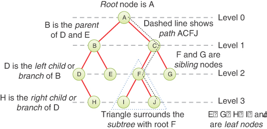
FIGURE 8-2 Tree terms
Root
The node at the top of the tree is called the root. There is only one root in a tree, labeled A in the figure.
Path
Think of someone walking from node to node along the edges that connect them. The resulting sequence of nodes is called a path. For a collection of nodes and edges to be defined as a tree, there must be one (and only one!) path from the root to any other node. Figure 8-3 shows a nontree. You can see that it violates this rule because there are multiple paths from A to nodes E and F. This is an example of a graph that is not a tree.

FIGURE 8-3 A nontree
Parent
Any node (except the root) has exactly one edge connecting it to a node above it. The node above it is called the parent of the node. The root node must not have a parent.
Child
Any node may have one or more edges connecting it to nodes below. These nodes below a given node are called its children, or sometimes, branches.
Sibling
Any node other than the root node may have sibling nodes. These nodes have a common parent node.
Leaf
A node that has no children is called a leaf node or simply a leaf. There can be only one root in a tree, but there can be many leaves. In contrast, a node that has children is an internal node.
Subtree
Any node (other than the root) may be considered to be the root of a subtree, which also includes its children, and its children’s children, and so on. If you think in terms of families, a node’s subtree contains all its descendants.
Visiting
A node is visited when program control arrives at the node, usually for the purpose of carrying out some operation on the node, such as checking the value of one of its data fields or displaying it. Merely passing over a node on the path from one node to another is not considered to be visiting the node.
Traversing
To traverse a tree means to visit all the nodes in some specified order. For example, you might visit all the nodes in order of ascending key value. There are other ways to traverse a tree, as we’ll describe later.
Levels
The level of a particular node refers to how many generations the node is from the root. If you assume the root is Level 0, then its children are at Level 1, its grandchildren are at Level 2, and so on. This is also sometimes called the depth of a node.
Keys
You’ve seen that one data field in an object is usually designated as a key value, or simply a key. This value is used to search for the item or perform other operations on it. In tree diagrams, when a circle represents a node holding a data item, the key value of the item is typically shown in the circle.
Binary Trees
If every node in a tree has at most two children, the tree is called a binary tree. In this chapter we focus on binary trees because they are the simplest and the most common.
The two children of each node in a binary tree are called the left child and the right child, corresponding to their positions when you draw a picture of a tree, as shown in Figure 8-2. A node in a binary tree doesn’t necessarily have the maximum of two children; it may have only a left child or only a right child, or it can have no children at all (in which case it’s a leaf).
Binary Search Trees
The kind of binary tree we discuss at the beginning of this chapter is technically called a binary search tree. The keys of the nodes have a particular ordering in search trees. Figure 8-4 shows a binary search tree.
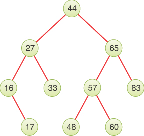
FIGURE 8-4 A binary search tree
Note
The defining characteristic of a binary search tree is this: a node’s left child must have a key less than its parent’s key, and a node’s right child must have a key greater than or equal to that of its parent.
An Analogy
One commonly encountered tree is the hierarchical file system on desktop computers. This system was modeled on the prevailing document storage technology used by businesses in the twentieth century: filing cabinets containing folders that in turn contained subfolders, down to individual documents. Computer operating systems mimic that by having files stored in a hierarchy. At the top of the hierarchy is the root directory. That directory contains “folders,” which are subdirectories, and files, which are like the paper documents. Each subdirectory can have subdirectories of its own and more files. These all have analogies in the tree: the root directory is the root node, subdirectories are nodes with children, and files are leaf nodes.
To specify a particular file in a file system, you use the full path from the root directory down to the file. This is the same as the path to a node of a tree. Uniform resource locators (URLs) use a similar construction to show a path to a resource on the Internet. Both file system pathnames and URLs allow for many levels of subdirectories. The last name in a file system path is either a subdirectory or a file. Files represent leaves; they have no children of their own.
Clearly, a hierarchical file system is not a binary tree because a directory may have many children. A hierarchical file system differs in another significant way from the trees that we discuss here. In the file system, subdirectories contain no data other than attributes like their name; they contain only references to other subdirectories or to files. Only files contain data. In a tree, every node contains data. The exact type of data depends on what’s being represented: records about personnel, records about components used to construct a vehicle, and so forth. In addition to the data, all nodes except leaves contain references to other nodes.
Hierarchical file systems differ from binary search trees in other aspects, too. The purpose of the file system is to organize files; the purpose of a binary search tree is more general and abstract. It’s a data structure that provides the common operations of insertion, deletion, search, and traversal on a collection of items, organizing them by their keys to speed up the operations. The analogy between the two is meant to show another familiar system that shares some important characteristics, but not all.
How Do Binary Search Trees Work?
Let’s see how to carry out the common binary tree operations of finding a node with a given key, inserting a new node, traversing the tree, and deleting a node. For each of these operations, we first show how to use the Binary Search Tree Visualization tool to carry it out; then we look at the corresponding Python code.
The Binary Search Tree Visualization Tool
For this example, start the Binary Search Tree Visualization tool (the program is called BinaryTree.py). You should see a screen something like that shown in Figure 8-5.
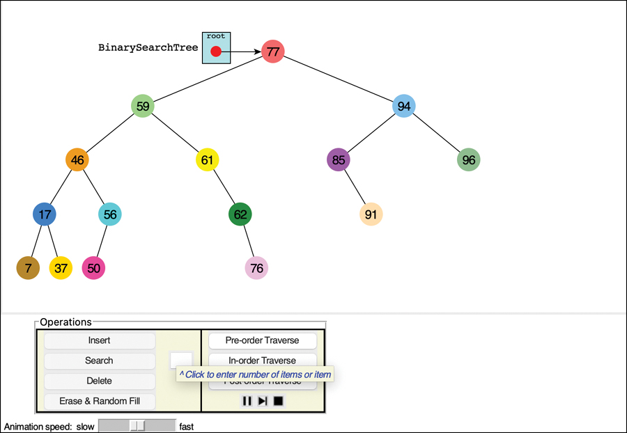
FIGURE 8-5 The Binary Search Tree Visualization tool
Using the Visualization Tool
The key values shown in the nodes range from 0 to 99. Of course, in a real tree, there would probably be a larger range of key values. For example, if telephone numbers were used for key values, they could range up to 999,999,999,999,999 (15 digits including country codes in the International Telecommunication Union standard). We focus on a simpler set of possible keys.
Another difference between the Visualization tool and a real tree is that the tool limits its tree to a depth of five; that is, there can be no more than five levels from the root to the bottom (level 0 through level 4). This restriction ensures that all the nodes in the tree will be visible on the screen. In a real tree the number of levels is unlimited (until the computer runs out of memory).
Using the Visualization tool, you can create a new tree whenever you want. To do this, enter a number of items and click the Erase & Random Fill button. You can ask to fill with 0 to 99 items. If you choose 0, you will create an empty tree. Using larger numbers will fill in more nodes, but some of the requested nodes may not appear. That’s due to the limit on the depth of the tree and the random order the items are inserted. You can experiment by creating trees with different numbers of nodes to see the variety of trees that come out of the random sequencing.
The nodes are created with different colors. The color represents the data stored with the key. We show a little later how that data is updated in some operations.
Constructing Trees
As shown in the Visualization tool, the tree’s shape depends both on the items it contains as well as the order the items are inserted into the tree. That might seem strange at first. If items are inserted into a sorted array, they always end up in the same order, regardless of their sequencing. Why are binary search trees different?
One of the key features of the binary search tree is that it does not have to fully order the items as they are inserted. When it adds a new item to an existing tree, it decides where to place the new leaf node by comparing its key with that of the nodes already stored in the tree. It follows a path from the root down to a missing child where the new node “belongs.” By choosing the left child when the new node’s key is less than the key of an internal node and the right child for other values, there will always be a unique path for the new node. That unique path means you can easily find that node by its key later, but it also means that the previously inserted items affect the path to any new item.
For example, if you start with an empty binary search tree and insert nodes in increasing key order, the unique path for each one will always be the rightmost path. Each insertion adds one more node at the bottom right. If you reverse the order of the nodes and insert them into an empty tree, each insertion will add the node at the bottom left because the key is lower than any other in the tree so far. Figure 8-6 shows what happens if you insert nodes with keys 44, 65, 83, and 87 in forward or reverse order.

FIGURE 8-6 Trees made by inserting nodes in sorted order
Unbalanced Trees
The trees shown in Figure 8-6, don’t look like trees. In fact, they look more like linked lists. One of the goals for a binary search tree is to speed up the search for a particular node, so having to step through a linked list to find the node would not be an improvement. To get the benefit of the tree, the nodes should be roughly balanced on both sides of the root. Ideally, each step along the path to find a node should cut the number of nodes to search in half, just like in binary searches of arrays and the guess-a-number game described in Chapter 2.
We can call some trees unbalanced; that is, they have most of their nodes on one side of the root or the other, as shown in Figure 8-7. Any subtree may also be unbalanced like the outlined one on the lower left of the figure. Of course, only a fully balanced tree will have equal numbers of nodes on the left and right subtrees (and being fully balanced, every node’s subtree will be fully balanced too). Inserting nodes one at a time on randomly chosen items means most trees will be unbalanced by one or more nodes as they are constructed, so you typically cannot expect to find fully balanced trees. In the following chapters, we look more carefully at ways to balance them as nodes are inserted and deleted.

FIGURE 8-7 An unbalanced tree (with an unbalanced subtree)
Trees become unbalanced because of the order in which the data items are inserted. If these key values are inserted randomly, the tree will be more or less balanced. When an ascending sequence (like 11, 18, 33, 42, 65) or a descending sequence is encountered, all the values will be right children (if ascending) or left children (if descending), and the tree will be unbalanced. The key values in the Visualization tool are generated randomly, but of course some short ascending or descending sequences will be created anyway, which will lead to local imbalances.
If a tree is created by data items whose key values arrive in random order, the problem of unbalanced trees may not be too much of a problem for larger trees because the chances of a long run of numbers in a sequence is small. Sometimes, however, key values will arrive in strict sequence; for example, when someone doing data entry arranges a stack of forms into alphabetical order by name before entering the data. When this happens, tree efficiency can be seriously degraded. We discuss unbalanced trees and what to do about them in Chapters 9 and 10.
Representing the Tree in Python Code
Let’s start implementing a binary search tree in Python. As with other data structures, there are several approaches to representing a tree in the computer’s memory. The most common is to store the nodes at (unrelated) locations in memory and connect them using references in each node that point to its children.
You can also represent a tree in memory as an array, with nodes in specific positions stored in corresponding positions in the array. We return to this possibility at the end of this chapter. For our sample Python code we’ll use the approach of connecting the nodes using references, similar to the way linked lists were implemented in Chapter 5.
The BinarySearchTree Class
We need a class for the overall tree object: the object that holds, or at least leads to, all the nodes. We’ll call this class BinarySearchTree. It has only one field, __root, that holds the reference to the root node, as shown in Listing 8-1. This is very similar to the LinkedList class that was used in Chapter 5 to represent linked lists. The BinarySearchTree class doesn’t need fields for the other nodes because they are all accessed from the root node by following other references.
LISTING 8-1 The Constructor for the BinarySearchTree Class

class BinarySearchTree(object): # A binary search tree class

   def __init__(self):          # The tree organizes nodes by their
      self.__root = None        # keys. Initially, it is empty.
The constructor initializes the reference to the root node as None to start with an empty tree. When the first node is inserted, __root will point to it as shown in the Visualization tool example of Figure 8-5. There are, of course, many methods that operate on BinarySearchTree objects, but first, you need to define the nodes inside them.
The __Node Class
The nodes of the tree contain the data representing the objects being stored (contact information in an address book, for example), a key to identify those objects (and to order them), and the references to each of the node’s two children. To remind us that callers that create BinarySearchTree objects should not be allowed to directly alter the nodes, we make a private __Node class inside that class. Listing 8-2 shows how an internal class can be defined inside the BinarySearchTree class.
LISTING 8-2 The Constructors for the __Node and BinarySearchTree Classes

class BinarySearchTree(object):  # A binary search tree class
…

   class __Node(object):         # A node in a binary search tree
      def __init__(              # Constructor takes a key that is
            self,                # used to determine the position
            key,                 # inside the search tree,
            data,                # the data associated with the key
            left=None,           # and a left and right child node
            right=None):         # if known
         self.key  = key         # Copy parameters to instance
         self.data = data        # attributes of the object
         self.leftChild = left
         self.rightChild = right

      def __str__(self):         # Represent a node as a string
         return "{" + str(self.key) + ", " + str(self.data) + "}"

   def __init__(self):           # The tree organizes nodes by their
      self.__root = None         # keys. Initially, it is empty.

   def isEmpty(self):            # Check for empty tree
      return self.__root is None

   def root(self):               # Get the data and key of the root node
      if self.isEmpty():         # If the tree is empty, raise exception
         raise Exception("No root node in empty tree")
      return (                   # Otherwise return root data and its key
         self.__root.data, self.__root.key)
The __Node objects are created and manipulated by the BinarySearchTree’s methods. The fields inside __Node can be initialized as public attributes because the BinarySearchTree‘s methods take care never to return a __Node object. This declaration allows for direct reading and writing without making accessor methods like getKey() or setData(). The __Node constructor simply populates the fields from the arguments provided. If the child nodes are not provided, the fields for their references are filled with None.
We add a __str__() method for __Node objects to aid in displaying the contents while debugging. Notably, it does not show the child nodes. We discuss how to display full trees a little later. That’s all the methods needed for __Node objects; all the rest of the methods you define are for BinarySearchTree objects.
Listing 8-2 shows an isEmpty() method for BinarySearchTree objects that checks whether the tree has any nodes in it. The root() method extracts the root node’s data and key. It’s like peek() for a queue and raises an exception if the tree is empty.
Some programmers also include a reference to a node’s parent in the __Node class. Doing so simplifies some operations but complicates others, so we don’t include it here. Adding a parent reference achieves something similar to the DoublyLinkedList class described in Chapter 5, “Linked Lists”; it’s useful in certain contexts but adds complexity.
We’ve made another design choice by storing the key for each node in its own field. For the data structures based on arrays, we chose to use a key function that extracts the key from each array item. That approach was more convenient for arrays because storing the keys separately from the data would require the equivalent of a key array along with the data array. In the case of node class with named fields, adding a key field makes the code perhaps more readable and somewhat more efficient by avoiding some function calls. It also makes the key more independent of the data, which adds flexibility and can be used to enforce constraints like immutable keys even when data changes.
The BinarySearchTree class has several methods. They are used for finding, inserting, deleting, and traversing nodes; and for displaying the tree. We investigate them each separately.
Finding a Node
Finding a node with a specific key is the simplest of the major tree operations. It’s also the most important because it is essential to the binary search tree’s purpose.
The Visualization tool shows only the key for each node and a color for its data. Keep in mind that the purpose of the data structure is to store a collection of records, not just the key or a simple color. The keys can be more than simple integers; any data type that can be ordered could be used. The Visualization and examples shown here use integers for brevity. After a node is discovered by its key, it’s the data that’s returned to the caller, not the node itself.
Using the Visualization Tool to Find a Node
Look at the Visualization tool and pick a node, preferably one near the bottom of the tree (as far from the root as possible). The number shown in this node is its key value. We’re going to demonstrate how the Visualization tool finds the node, given the key value.
For purposes of this discussion, we choose to find the node holding the item with key value 50, as shown in Figure 8-8. Of course, when you run the Visualization tool, you may get a different tree and may need to pick a different key value.
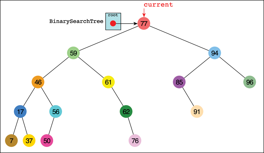
FIGURE 8-8 Finding the node with key 50
Enter the key value in the text entry box, hold down the Shift key, and select the Search button, and then the Step button,  . By repeatedly pressing the Step button, you can see all the individual steps taken to find key 50. On the second press, the
 current pointer shows up at the root of the tree, as seen in Figure 8-8. On the next click, a parent pointer shows up that will follow the current pointer. Ignore that pointer and the code display for a moment; we describe them in detail shortly.
As the Visualization tool looks for the specified node, it makes a decision at the current node. It compares the desired key with the one found at the current node. If it’s the same, it’s found the desired node and can quit. If not, it must decide where to look next.
In Figure 8-8 the current arrow starts at the root. The program compares the goal key value 50 with the value at the root, which is 77. The goal key is less, so the program knows the desired node must be on the left side of the tree—either the root’s left child or one of that child’s descendants. The left child of the root has the value 59, so the comparison of 50 and 59 will show that the desired node is in the left subtree of 59. The current arrow goes to 46, the root of that subtree. This time, 50 is greater than the 46 node, so it goes to the right, to node 56, as shown in Figure 8-9. A few steps later, comparing 50 with 56 leads the program to the left child. The comparison at that leaf node shows that 50 equals the node’s key value, so it has found the node we sought.

FIGURE 8-9 The second to last step in finding key 50
The Visualization tool changes a little after it finds the desired node. The current arrow changes into the node arrow (and parent changes into p). That’s because of the way variables are named in the code, which we show in the next section. The tool doesn’t do anything with the node after finding it, except to encircle it and display a message saying it has been found. A serious program would perform some operation on the found node, such as displaying its contents or changing one of its fields.
Python Code for Finding a Node
Listing 8-3 shows the code for the __find() and search() methods. The __find() method is private because it can return a node object. Callers of the BinarySearchTree class use the search() method to get the data stored in a node.
LISTING 8-3 The Methods to Find a Binary Search Tree Node Based on Its Key
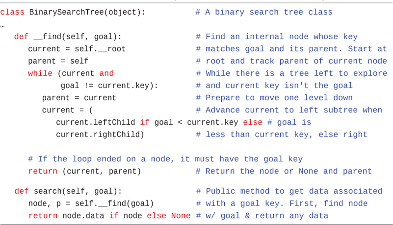
class BinarySearchTree(object):            # A binary search tree class
…
   def __find(self, goal):                 # Find an internal node whose key
      current = self.__root                # matches goal and its parent. Start at
      parent = self                        # root and track parent of current node
      while (current and                   # While there is a tree left to explore
             goal != current.key):         # and current key isn't the goal
          parent = current                 # Prepare to move one level down
          current = (                      # Advance current to left subtree when
             current.leftChild if goal < current.key else # goal is
             current.rightChild)           # less than current key, else right

      # If the loop ended on a node, it must have the goal key
      return (current, parent)            # Return the node or None and parent

   def search(self, goal):                # Public method to get data associated
      node, p = self.__find(goal)         # with a goal key. First, find node
      return node.data if node else None  # w/ goal & return any data
The only argument to __find() is goal, the key value to be found. This routine creates the variable current to hold the node currently being examined. The routine starts at the root – the only node it can access directly. That is, it sets current to the root. It also sets a parent variable to self, which is the tree object. In the Visualization tool, parent starts off pointing at the tree object. Because parent links are not stored in the nodes, the __find() method tracks the parent node of current so that it can return it to the caller along with the goal node. This capability will be very useful in other methods. The parent variable is always either the BinarySearchTree being searched or one of its __Node objects.
In the while loop, __find() first confirms that current is not None and references some existing node. If it doesn’t, the search has gone beyond a leaf node (or started with an empty tree), and the goal node isn’t in the tree. The second part of the while test compares the value to be found, goal, with the value of the current node’s key field. If the key matches, then the loop is done. If it doesn’t, then current needs to advance to the appropriate subtree. First, it updates parent to be the current node and then updates current. If goal is less than current’s key, current advances to its left child. If goal is greater than current’s key, current advances to its right child.
Can't Find the Node
If current becomes equal to None, you’ve reached the end of the line without finding the node you were looking for, so it can’t be in the tree. That could happen if the root node was None or if following the child links led to a node without a child (on the side where the goal key would go). Both the current node (None) and its parent are returned to the caller to indicate the result. In the Visualization tool, try entering a key that doesn’t appear in the tree and select Search. You then see the current pointer descend through the existing nodes and land on a spot where the key should be found but no node exists. Pointing to “empty space” indicates that the variable’s value is None.
Found the Node
If the condition of the while loop is not satisfied while current references some node in the tree, then the loop exits, and the current key must be the goal. That is, it has found the node being sought and current references it. It returns the node reference along with the parent reference so that the routine that called __find() can access any of the node’s (or its parent’s) data. Note that it returns the value of current for both success and failure of finding the key; it is None when the goal isn’t found.
The search() method calls the __find() method to set its node and parent (p) variables. That’s what you see in the Visualization tool after the __find() method returns. If a non-None reference was found, search() returns the data for that node. In this case, the method assumes that data items stored in the nodes can never be None; otherwise, the caller would not be able to distinguish them.
Tree Efficiency
As you can see, the time required to find a node depends on its depth in the tree, the number of levels below the root. If the tree is balanced, this is O(log N) time, or more specifically O(log2 N) time, the logarithm to base 2, where N is the number of nodes. It’s just like the binary search done in arrays where half the nodes were eliminated after each comparison. A fully balanced tree is the best case. In the worst case, the tree is completely unbalanced, like the examples shown in Figure 8-6, and the time required is O(N). We discuss the efficiency of __find() and other operations toward the end of this chapter.
Inserting a Node
To insert a node, you must first find the place to insert it. This is the same process as trying to find a node that turns out not to exist, as described in the earlier “Can’t Find the Node” section. You follow the path from the root toward the appropriate node. This is either a node with the same key as the node to be inserted or None, if this is a new key. If it’s the same key, you could try to insert it in the right subtree, but doing so adds some complexity. Another option is to replace the data for that node with the new data. For now, we allow only unique keys to be inserted; we discuss duplicate keys later.
If the key to insert is not in the tree, then __find() returns None for the reference to the node along with a parent reference. The new node is connected as the parent’s left or right child, depending on whether the new node’s key is less or greater than that of the parent. If the parent reference returned by __find() is self, the BinarySearchTree itself, then the node becomes the root node.
Figure 8-10 illustrates the process of inserting a node, with key 31, into a tree. The __find(31) method starts walking the path from the root node. Because 31 is less than the root node key, 44, it follows the left child link. That child’s key is 27, so it follows that child’s right child link. There it encounters key 33, so it again follows the left child link. That is None, so __find(31) stops with the parent pointing at the leaf node with key 33. The new leaf node with key 31 is created, and the parent’s left child link is set to reference it.

FIGURE 8-10 Inserting a node in binary search tree
Using the Visualization Tool to Insert a Node
To insert a new node with the Visualization tool, enter a key value that’s not in the tree and select the Insert button. The first step for the program is to find where it should be inserted. For example, inserting 81 into the tree from an earlier example calls the __find() method of Listing 8-3, which causes the search to follow the path shown in Figure 8-11.
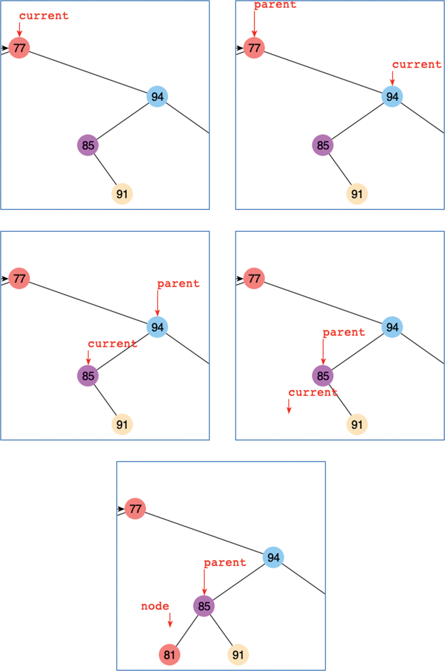
FIGURE 8-11 Steps for inserting a node with key 81 using the Visualization tool
The current pointer starts at the root node with key 77. Finding 81 to be larger, it goes to the right child, node 94. Now the key to insert is less than the current key, so it descends to node 85. The parent pointer follows the current pointer at each of these steps. When current reaches node 85, it goes to its left child and finds it missing. The call to __find() returns None and the parent pointer.
After locating the parent node with the empty child where the new key should go, the Visualization tool creates a new node with the key 81, some data represented by a color, and sets the left child pointer of node 85, the parent, to point at it. The node pointer returned by __find() is moved away because it still is None.
Python Code for Inserting a Node
The insert() method takes parameters for the key and data to insert, as shown in Listing 8-4. It calls the __find() method with the new node’s key to determine whether that key already exists and where its parent node should be. This implementation allows only unique keys in the tree, so if it finds a node with the same key, insert() updates the data for that key and returns False to indicate that no new node was created.
LISTING 8-4 The insert() Method of BinarySearchTree
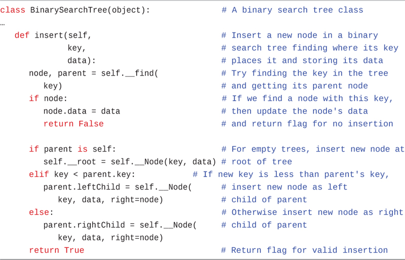
class BinarySearchTree(object):               # A binary search tree class
…
   def insert(self,                           # Insert a new node in a binary
              key,                            # search tree finding where its key
              data):                          # places it and storing its data
      node, parent = self.__find(             # Try finding the key in the tree
         key)                                 # and getting its parent node
      if node:                                # If we find a node with this key,
         node.data = data                     # then update the node's data
         return False                         # and return flag for no insertion

      if parent is self:                      # For empty trees, insert new node at
         self.__root = self.__Node(key, data) # root of tree
      elif key < parent.key:            # If new key is less than parent's key,
         parent.leftChild = self.__Node(      # insert new node as left
            key, data, right=node)            # child of parent
      else:                                   # Otherwise insert new node as right
         parent.rightChild = self.__Node(     # child of parent
            key, data, right=node)
      return True                             # Return flag for valid insertion
If a matching node was not found, then insertion depends on what kind of parent reference was returned from __find(). If it’s self, the BinarySearchTree must be empty, so the new node becomes the root node of the tree. Otherwise, the parent is a node, so insert() decides which child will get the new node by comparing the new node’s key with that of the parent. If the new key is lower, then the new node becomes the left child; otherwise, it becomes the right child. Finally, insert() returns True to indicate the insertion succeeded.
When insert() creates the new node, it sets the new node’s right child to the node returned from __find(). You might wonder why that’s there, especially because node can only be None at that point (if it were not None, insert() would have returned False before reaching that point). The reason goes back to what to do with duplicate keys. If you allow nodes with duplicate keys, then you must put them somewhere. The binary search tree definition says that a node’s key is less than or equal to that of its right child. So, if you allow duplicate keys, the duplicate node cannot go in the left child. By specifying something other than None as the right child of the new node, other nodes with the same key can be retained. We leave as an exercise how to insert (and delete) nodes with duplicate keys.
Traversing the Tree
Traversing a tree means visiting each node in a specified order. Traversing a tree is useful in some circumstances such as going through all the records to look for ones that need some action (for example, parts of a vehicle that are sourced from a particular country). This process may not be as commonly used as finding, inserting, and deleting nodes but it is important nevertheless.
You can traverse a tree in three simple ways. They’re called pre-order, in-order, and post-order. The most commonly used order for binary search trees is in-order, so let’s look at that first and then return briefly to the other two.
In-order Traversal
An in-order traversal of a binary search tree causes all the nodes to be visited in ascending order of their key values. If you want to create a list of the data in a binary tree sorted by their keys, this is one way to do it.
The simplest way to carry out a traversal is the use of recursion (discussed in Chapter 6). A recursive method to traverse the entire tree is called with a node as an argument. Initially, this node is the root. The method needs to do only three things:
Call itself to traverse the node’s left subtree.
Visit the node.
Call itself to traverse the node’s right subtree.
Remember that visiting a node means doing something to it: displaying it, updating a field, adding it to a queue, writing it to a file, or whatever.
The three traversal orders work with any binary tree, not just with binary search trees. The traversal mechanism doesn’t pay any attention to the key values of the nodes; it only concerns itself with the node’s children and data. In other words, in-order traversal means “in order of increasing key values” only when the binary search tree criteria are used to place the nodes in the tree. The in of in-order refers to a node being visited in between the left and right subtrees. The pre of pre-order means visiting the node before visiting its children, and post-order visits the node after visiting the children. This distinction is like the differences between infix and postfix notation for arithmetic expressions described in Chapter 4, “Stacks and Queues.”
To see how this recursive traversal works, Figure 8-12 shows the calls that happen during an in-order traversal of a small binary tree. The tree variable references a four-node binary search tree. The figure shows the invocation of an inOrderTraverse() method on the tree that will call the print function on each of its nodes.
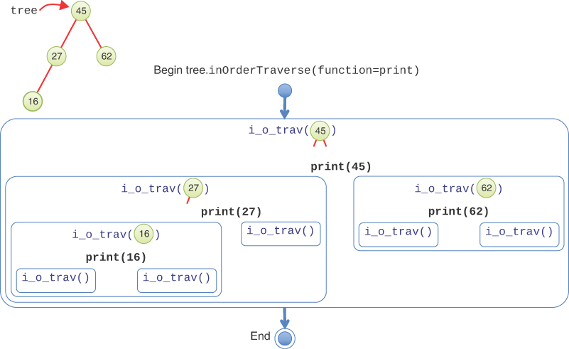
FIGURE 8-12 In-order traversal of a small tree
The blue rounded rectangles show the recursive calls on each subtree. The name of the recursive method has been abbreviated as i_o_trav() to fit all the calls in the figure. The first (outermost) call is on the root node (key 45). Each recursive call performs the three steps outlined previously. First, it makes a recursive call on the left subtree, rooted at key 27. That shows up as another blue rounded rectangle on the left of the figure.
Processing the subtree rooted at key 27 starts by making a recursive call on its left subtree, rooted at key 16. Another rectangle shows that call in the lower left. As before, its first task is to make a recursive call on its left subtree. That subtree is empty because it is a leaf node and is shown in the figure as a call to i_o_trav() with no arguments. Because the subtree is empty, nothing happens and the recursive call returns.
Back in the call to i_o_trav(16), it now reaches step 2 and “visits” the node by executing the function, print, on the node itself. This is shown in the figure as print(16) in black. In general, visiting a node would do more than just print the node’s key; it would take some action on the data stored at the node. The figure doesn’t show that action, but it would occur when the print(16) is executed.
After visiting the node with key 16, it’s time for step 3: call itself on the right subtree. The node with key 16 has no right child, which shows up as the smallest-sized rectangle because it is a call on an empty subtree. That completes the execution for the subtree rooted at key 16. Control passes back to the caller, the call on the subtree rooted at key 27.
The rest of the processing progresses similarly. The visit to the node with key 27 executes print(27) and then makes a call on its empty right subtree. That finishes the call on node 27 and control passes back to the call on the root of the tree, node 45. After executing print(45), it makes a call to traverse its right (nonempty) subtree. This is the fourth and final node in the tree, node 62. It makes a call on its empty left subtree, executes print(62), and finishes with a call on its empty right subtree. Control passes back up through the call on the root node, 45, and that ends the full tree traversal.
Pre-order and Post-order Traversals
The other two traversal orders are similar: only the sequence of visiting the node changes. For pre-order traversal, the node is visited first, and for post-order, it’s visited last. The two subtrees are always visited in the same order: left and then right. Figure 8-13 shows the execution of a pre-order traversal on the same four-node tree as in Figure 8-12. The execution of the print() function happens before visiting the two subtrees. That means that the pre-order traversal would print 45, 27, 16, 62 compared to the in-order traversal’s 16, 27, 45, 62. As the figures show, the differences between the orders are small, but the overall effect is large.
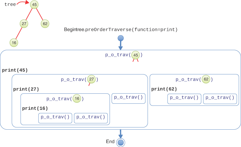
FIGURE 8-13 Pre-order traversal of a small tree
Python Code for Traversing
Let’s look at a simple way of implementing the in-order traversal now. As you saw in stacks, queues, linked lists, and other data structures, it’s straightforward to define the traversal using a function passed as an argument that gets applied to each item stored in the structure. The interesting difference with trees is that recursion makes it very compact.
Because these trees are represented using two classes, BinarySearchTree and __Node, you need methods that can operate on both types of objects. In Listing 8-5, the inOrderTraverse() method handles the traversal on BinarySearchTree objects. It serves as the public interface to the traversal and calls a private method __inOrderTraverse() to do the actual work on subtrees. It passes the root node to the private method and returns.
LISTING 8-5 Recursive Implementation of inOrderTraverse()
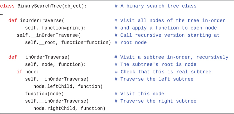
class BinarySearchTree(object):          # A binary search tree class
…
   def inOrderTraverse(                  # Visit all nodes of the tree in-order
         self, function=print):          # and apply a function to each node
      self.__inOrderTraverse(            # Call recursive version starting at
         self.__root, function=function) # root node

   def __inOrderTraverse(                # Visit a subtree in-order, recursively
         self, node, function):          # The subtree's root is node
      if node:                           # Check that this is real subtree
         self.__inOrderTraverse(         # Traverse the left subtree
            node.leftChild, function)
         function(node)                  # Visit this node
         self.__inOrderTraverse(         # Traverse the right subtree
            node.rightChild, function)
The private method expects a __Node object (or None) for its node parameter and performs the three steps on the subtree rooted at the node. First, it checks node and returns immediately if it is None because that signifies an empty subtree. For legitimate nodes, it first makes a recursive call to itself to process the left child of the node. Second, it visits the node by invoking the function on it. Third, it makes a recursive call to process the node’s right child. That’s all there is to it.
Using a Generator for Traversal
The inOrderTraverse() method is straightforward, but it has at least three shortcomings. First, to implement the other orderings, you would either need to write more methods or add a parameter that specifies the ordering to perform.
Second, the function passed as an argument to “visit” each node needs to take a __Node object as argument. That’s a private class inside the BinarySearchTree that protects the nodes from being manipulated by the caller. One alternative that avoids passing a reference to a __Node object would be to pass in only the data field (and maybe the key field) of each node as arguments to the visit function. That approach would minimize what the caller could do to the node and prevent it from altering the other node references.
Third, using a function to describe the action to perform on each node has its limitations. Typically, functions perform the same operation each time they are invoked and don’t know about the history of previous calls. During the traversal of a data structure like a tree, being able to make use of the results of previous node visits dramatically expands the possible operations. Here are some examples that you might want to do:
 Add up all the values in a particular field at every node.
- Get a list of all the unique strings in a field from every node.
- Add the node’s key to some list if none of the previously visited nodes have a bigger value in some field.
In all these traversals, it’s very convenient to be able to accumulate results somewhere during the traversal. That’s possible to do with functions, but generators make it easier. We introduced generators in Chapter 5, and because trees share many similarities with those structures, they are very useful for traversing trees.
We address these shortcomings in a recursive generator version of the traverse method, traverse_rec(), shown in Listing 8-6. This version adds some complexity to the code but makes using traversal much easier. First, we add a parameter, traverseType, to the traverse_rec() method so that we don’t need three separate traverse routines. The first if statement verifies that this parameter is one of the three supported orderings: pre, in, and post. If not, it raises an exception. Otherwise, it launches the recursive private method, __traverse(), starting with the root node, just like inOrderTraverse() does.
There is an important but subtle point to note in calling the __traverse() method. The public traverse_rec() method returns the result of calling the private __traverse() method and does not just simply call it as a subroutine. The reason is that the traverse() method itself is not the generator; it has no yield statements. It must return the iterator produced by the call to __traverse(), which will be used by the traverse_rec() caller to iterate over the nodes.
Inside the __traverse() method, there are a series of if statements. The first one tests the base case. If node is None, then this is an empty tree (or subtree). It returns to indicate the iterator has hit the end (which Python converts to a StopIteration exception). The next if statement checks whether the traversal type is pre-order, and if it is, it yields the node’s key and data. Remember that the iterator will be paused at this point while control passes back to its caller. That is where the node will be “visited.” After the processing is done, the caller’s loop invokes this iterator to get the next node. The iterator resumes processing right after the yield statement, remembering all the context.
When the iterator resumes (or if the order was something other than pre-order), the next step is a for loop. This is a recursive generator to perform the traversal of the left subtree. It calls the __traverse() method on the node’s leftChild using the same traverseType. That creates its own iterator to process the nodes in that subtree. As nodes are yielded back as key, data pairs, this higher-level iterator yields them back to its caller. This loop construction produces a nested stack of iterators, similar to the nested invocations of i_o_trav() shown in Figure 8-12. When each iterator returns at the end of its work, it raises a StopIteration. The enclosing iterator catches each exception, so the various levels don’t interfere with one another.
LISTING 8-6 The Recursive Generator for Traversal
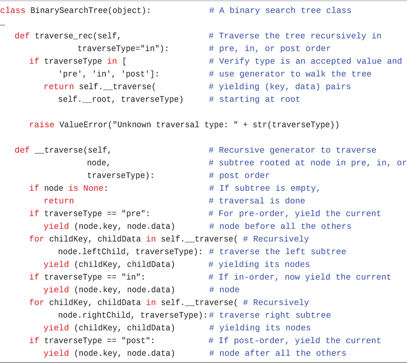
class BinarySearchTree(object):            # A binary search tree class
…
   def traverse_rec(self,                  # Traverse the tree recursively in
                traverseType="in"):        # pre, in, or post order
      if traverseType in [                 # Verify type is an accepted value and
            'pre', 'in', 'post']:          # use generator to walk the tree
         return self.__traverse(           # yielding (key, data) pairs
            self.__root, traverseType)     # starting at root

      raise ValueError("Unknown traversal type: " + str(traverseType))

   def __traverse(self,                    # Recursive generator to traverse
                  node,                    # subtree rooted at node in pre, in, or
                  traverseType):           # post order
      if node is None:                     # If subtree is empty,
         return                            # traversal is done
      if traverseType == "pre":            # For pre-order, yield the current
         yield (node.key, node.data)       # node before all the others
      for childKey, childData in self.__traverse( # Recursively
            node.leftChild, traverseType):  # traverse the left subtree
         yield (childKey, childData)          # yielding its nodes
      if traverseType == "in":             # If in-order, now yield the current
         yield (node.key, node.data)       # node
      for childKey, childData in self.__traverse( # Recursively
            node.rightChild, traverseType):# traverse right subtree
         yield (childKey, childData)       # yielding its nodes
      if traverseType == "post":           # If post-order, yield the current
         yield (node.key, node.data)       # node after all the others
The rest of the __traverse() method is straightforward. After finishing the loop over all the nodes in the left subtree, the next if statement checks for the in-order traversal type and yields the node’s key and data, if that’s the ordering. The node gets processed between the left and right subtrees for an in-order traversal. After that, the right subtree is processed in its own loop, yielding each of the visited nodes back to its caller. After the right subtree is done, a check for post-order traversal determines whether the node should be yielded at this stage or not. After that, the __traverse() generator is done, ending its caller’s loop.
Making the Generator Efficient
The recursive generator has the advantage of structural simplicity. The base cases and recursive calls follow the node and child structure of the tree. Developing the prototype and proving its correct behavior flow naturally from this structure.
The generator does, however, suffer some inefficiency in execution. Each invocation of the __traverse() method invokes two loops: one for the left and one for the right child. Each of those loops creates a new iterator to yield the items from their subtrees back through the iterator created by this invocation of the __traverse() method itself. That layering of iterators extends from the root down to each leaf node.
Traversing the N items in the tree should take O(N) time, but creating a stack of iterators from the root down to each leaf adds complexity that’s proportional to the depth of the leaves. The leaves are at O(log N) depth, in the best case. That means the overall traversal of N items will take O(N×log N) time.
To achieve O(N) time, you need to apply the method discussed at the end of Chapter 6 and use a stack to hold the items being processed. The items include both Node structures and the (key, data) pairs stored at the nodes to be traversed in a particular order. Listing 8-7 shows the code.
The nonrecursive method combines the two parts of the recursive approach into a single traverse() method. The same check for the validity of the traversal type happens at the beginning. The next step creates a stack, using the Stack class built on a linked list from Chapter 5 (defined in the LinkStack module).
Initially, the method pushes the root node of the tree on the stack. That means the remaining work to do is the entire tree starting at the root. The while loop that follows works its way through the remaining work until the stack is empty.
At each pass through the while loop, the top item of the stack is popped off. Three kinds of items could be on the stack: a Node item, a (key, data) tuple, or None. The latter happens if the tree is empty and when it processes the leaf nodes (and finds their children are None).
If the top of the stack is a Node item, the traverse() method determines how to process the node’s data and its children based on the requested traversal order. It pushes items onto the stack to be processed on subsequent passes through the while loop. Because the items will be popped off the stack in the reverse order from the way they were pushed onto it, it starts by handling the case for post-order traversal.
In post-order, the first item pushed is the node’s (key, data) tuple. Because it is pushed first, it will be processed last overall. The next item pushed is the node’s right child. In post-order, this is traversed just before processing the node’s data. For the other orders, the right child is always the last node processed.
After pushing on the right child, the next if statement checks whether the in-order traversal was requested. If so, it pushes the node’s (key, data) tuple on the stack to be processed in-between the two child nodes. That’s followed by pushing the left child on the stack for processing.
LISTING 8-7 The Nonrecursive traverse() Generator
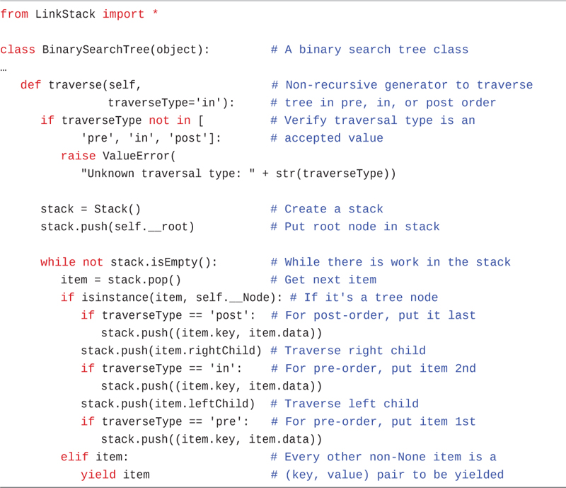
from LinkStack import *

class BinarySearchTree(object):         # A binary search tree class
…
   def traverse(self,                   # Non-recursive generator to traverse
                traverseType='in'):     # tree in pre, in, or post order
      if traverseType not in [          # Verify traversal type is an
            'pre', 'in', 'post']:       # accepted value
         raise ValueError(
            "Unknown traversal type: " + str(traverseType))

      stack = Stack()                   # Create a stack
      stack.push(self.__root)           # Put root node in stack

      while not stack.isEmpty():        # While there is work in the stack
         item = stack.pop()             # Get next item
         if isinstance(item, self.__Node): # If it's a tree node
            if traverseType == 'post':  # For post-order, put it last
               stack.push((item.key, item.data))
            stack.push(item.rightChild) # Traverse right child
            if traverseType == 'in':    # For pre-order, put item 2nd
               stack.push((item.key, item.data))
            stack.push(item.leftChild)  # Traverse left child
            if traverseType == 'pre':   # For pre-order, put item 1st
               stack.push((item.key, item.data))
         elif item:                     # Every other non-None item is a
            yield item                  # (key, value) pair to be yielded
Finally, the last if statement checks whether the pre-order traversal was requested and then pushes the node’s data on the stack for processing before the left and right children. It will be popped off during the next pass through the while loop. That completes all the work for a Node item.
The final elif statement checks for a non-None item on the stack, which must be a (key, data) tuple. When the loop finds such a tuple, it yields it back to the caller. The yield statement ensures that the traverse() method becomes a generator, not a function.
The loop doesn’t have any explicit handling of the None values that get pushed on the stack for empty root and child links. The reason is that there’s nothing to do for them: just pop them off the stack and continue on to the remaining work.
Using the stack, you have now made an O(N) generator. Each node of the tree is visited exactly once, pushed on the stack, and later popped off. Its key-data pairs and child links are also pushed on and popped off exactly once. The ordering of the node visits and child links follows the requested traversal ordering. Using the stack and carefully reversing the items pushed onto it make the code slightly more complex to understand but improve the performance.
Using the Generator for Traversing
The generator approach (both recursive and stack-based) makes the caller’s loops easy. For example, if you want to collect all the items in a tree whose data is below the average data value, you could use two loops:
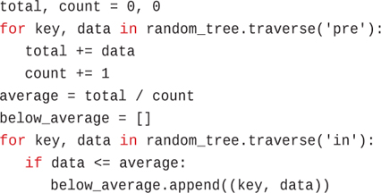
total, count = 0, 0
for key, data in random_tree.traverse('pre'):
   total += data
   count += 1
average = total / count
below_average = []
for key, data in random_tree.traverse('in'):
   if data <= average:
      below_average.append((key, data))
The first loop counts the number of items in random_tree and sums up their data values. The second loop finds all the items whose data is below the average and appends the key and data pair to the below_average list. Because the second loop is done in in-order, the keys in below_average are in ascending order. Being able to reference the variables that accumulate results—total, count, and below_average—without defining some global (or nonlocal) variables outside a function body, makes using the generator very convenient for traversal.
Traversing with the Visualization Tool
The Binary Search Tree Visualization tool allows you to explore the details of traversal using generators. You can launch any of the three kinds of traversals by selecting the Pre-order Traverse, In-order Traverse, or Post-order Traverse buttons. In each case, the tool executes a simple loop of the form
for key, data in tree.traverse("pre"):
   print(key)
To see the details, use the Step button (you can launch an operation in step mode by holding down the Shift key when selecting the button). In the code window, you first see the short traversal loop. The example calls the traverse() method to visit all the keys and data in a loop using one of the orders such as pre.
Figure 8-14 shows a snapshot near the beginning of a pre-order traversal. The code for the traverse() method appears at the lower right. To the right of the tree above the code, the stack is shown. The nodes containing keys 59 and 94 are on the stack. The top of the stack was already popped off and moved to the top right under the item label. It shows the key, 77, with a comma separating it from its colored rectangle to represent the (key, data) tuple that was pushed on the stack. The yield statement is highlighted, showing that the traverse() iterator is about to yield the key and data back to caller. The loop that called traverse() has scrolled off the code display but will be shown on the next step.
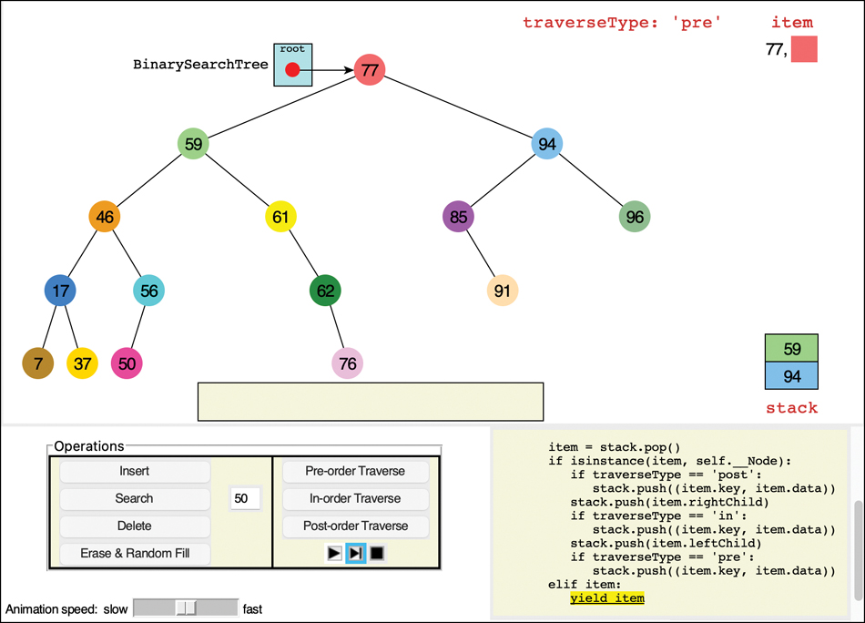
FIGURE 8-14 Traversing a tree in pre-order using the traverse() iterator
When control returns to the calling loop, the traverse() iterator disappears from the code window and so does the stack, as shown in Figure 8-15. The key and data variables are now bound to 77 and the root node’s data. The print statement is highlighted because the program is about to print the key in the output box along the bottom of the tree. The next step shows key 77 being copied to the output box.
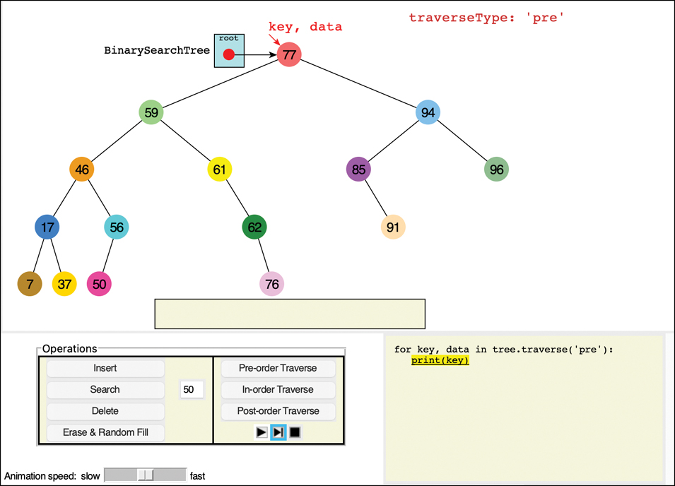
FIGURE 8-15 The loop calling the traverse() iterator
After printing, control returns to the for key, data in tree.traverse('pre') loop. That pushes the traverse() iterator back on the code display, along with its stack similar to Figure 8-14. The while loop in the iterator finds that the stack is not empty, so it pops off the top item. That item is node 59, the left child of node 77. The process repeats by pushing on node 59’s children and the node’s key, data pair on the stack. On the next loop iteration, that tuple is popped off the stack, and it is yielded back to the print loop.
The processing of iterators is complex to describe, and the Visualization tool makes it easier to follow the different levels and steps than reading a written description. Try stepping through the processing of several nodes, including when the iterator reaches a leaf node and pushes None on the stack. The stack guides the iterator to return to nodes that remain to be processed.
Traversal Order
What’s the point of having three traversal orders? One advantage is that in-order traversal guarantees an ascending order of the keys in binary search trees. There’s a separate motivation for pre- and post-order traversals. They are very useful if you’re writing programs that parse or analyze algebraic expressions. Let’s see why that is the case.
A binary tree (not a binary search tree) can be used to represent an algebraic expression that involves binary arithmetic operators such as +, –, /, and *. The root node and every nonleaf node hold an operator. The leaf nodes hold either a variable name (like A, B, or C) or a number. Each subtree is a valid algebraic expression.
For example, the binary tree shown in Figure 8-16 represents the algebraic expression

FIGURE 8-16 Binary tree representing an algebraic expression
(A+B) * C – D / E
This is called infix notation; it’s the notation normally used in algebra. (For more on infix and postfix, see the section “Parsing Arithmetic Expressions” in Chapter 4.) Traversing the tree in order generates the correct in-order sequence A+B*C–D/E, but you need to insert the parentheses yourself to get the expected order of operations. Note that subtrees form their own subexpressions like the (A+B) * C outlined in the figure.
What does all this have to do with pre-order and post-order traversals? Let’s see what’s involved in performing a pre-order traversal. The steps are
Visit the node.
Call itself to traverse the node’s left subtree.
Call itself to traverse the node’s right subtree.
Traversing the tree shown in Figure 8-16 using pre-order and printing the node’s value would generate the expression
–*+ABC/DE
This is called prefix notation. It may look strange the first time you encounter it, but one of its nice features is that parentheses are never required; the expression is unambiguous without them. Starting on the left, each operator is applied to the next two things to its right in the expression, called the operands. For the first operator, –, these two things are a product expression, *+ABC, and a division expression, /DE. For the second operator, *, the two things are a sum expression, +AB, and a single variable, C. For the third operator, +, the two things it operates on are the variables, A and B, so this last expression would be A+B in in-order notation. Finally, the fourth operator, /, operates on the two variables D and E.
The third kind of traversal, post-order, contains the three steps arranged in yet another way:
Call itself to traverse the node’s left subtree.
Call itself to traverse the node’s right subtree.
Visit the node.
For the tree in Figure 8-16, visiting the nodes with a post-order traversal generates the expression
AB+C*DE/–
This is called postfix notation. It means “apply the last operator in the expression, –, to the two things immediately to the left of it.” The first thing is AB+C*, and the second thing is DE/. Analyzing the first thing, AB+C*, shows its meaning to be “apply the * operator to the two things immediately to the left of it, AB+ and C.” Analyzing the first thing of that expression, AB+, shows its meaning to be “apply the + operator to the two things immediately to the left of it, A and B.” It’s hard to see initially, but the “things” are always one of three kinds: a single variable, a single number, or an expression ending in a binary operator.
To process the meaning of a postfix expression, you start from the last character on the right and interpret it as follows. If it’s a binary operator, then you repeat the process to interpret two subexpressions on its left, which become the operands of the operator. If it’s a letter, then it’s a simple variable, and if it’s a number, then it’s a constant. For both variables and numbers, you “pop” them off the right side of the expression and return them to the process of the enclosing expression.
We don’t show the details here, but you can easily construct a tree like that in Figure 8-16 by using a postfix expression as input. The approach is analogous to that of evaluating a postfix expression, which you saw in the PostfixTranslate.py program in Chapter 4 and its corresponding InfixCalculator Visualization tool. Instead of storing operands on the stack, however, you store entire subtrees. You read along the postfix string from left to right as you did in the PostfixEvaluate() method. Here are the steps when you encounter an operand (a variable or a number):
Make a tree with one node that holds the operand.
Push this tree onto the stack.
Here are the steps when you encounter an operator, O:
Pop two operand trees R and L off the stack (the top of the stack has the rightmost operand, R).
Create a new tree T with the operator, O, in its root.
Attach R as the right child of T.
Attach L as the left child of T.
Push the resulting tree, T, back on the stack.
When you’re done evaluating the postfix string, you pop the one remaining item off the stack. Somewhat amazingly, this item is a complete tree depicting the algebraic expression. You can then see the prefix and infix representations of the original postfix notation (and recover the postfix expression) by traversing the tree in one of the three orderings we described. We leave an implementation of this process as an exercise.
Finding Minimum and Maximum Key Values
Incidentally, you should note how easy it is to find the minimum and maximum key values in a binary search tree. In fact, this process is so easy that we don’t include it as an option in the Visualization tool. Still, understanding how it works is important.
For the minimum, go to the left child of the root; then go to the left child of that child, and so on, until you come to a node that has no left child. This node is the minimum. Similarly, for the maximum, start at the root and follow the right child links until they end. That will be the maximum key in the tree, as shown in Figure 8-17.

FIGURE 8-17 Minimum and maximum key values of a binary search tree
Here’s some code that returns the minimum node’s data and key values:
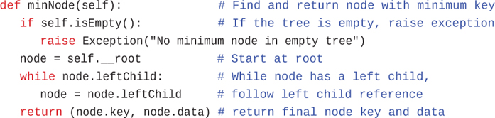
   def minNode(self):              # Find and return node with minimum key
      if self.isEmpty():           # If the tree is empty, raise exception
         raise Exception("No minimum node in empty tree")
      node = self.__root           # Start at root
      while node.leftChild:        # While node has a left child,
         node = node.leftChild     # follow left child reference
      return (node.key, node.data) # return final node key and data
Finding the maximum is similar; just swap the right for the left child. You learn about an important use of finding the minimum value in the next section about deleting nodes.
Deleting a Node
Deleting a node is the most complicated common operation required for binary search trees. The fundamental operation of deletion can’t be ignored, however, and studying the details builds character. If you’re not in the mood for character building, feel free to skip to the Efficiency of Binary Search Trees section.
You start by verifying the tree isn’t empty and then finding the node you want to delete, using the same approach you saw in __find() and insert(). If the node isn’t found, then you’re done. When you’ve found the node and its parent, there are three cases to consider:
The node to be deleted is a leaf (has no children).
The node to be deleted has one child.
The node to be deleted has two children.
Let’s look at these three cases in turn. The first is easy; the second, almost as easy; and the third, quite complicated.
Case 1: The Node to Be Deleted Has No Children
To delete a leaf node, you simply change the appropriate child field in the node’s parent to None instead of to the node. The node object still exists, but it is no longer part of the tree, as shown when deleting node 17 in Figure 8-18.
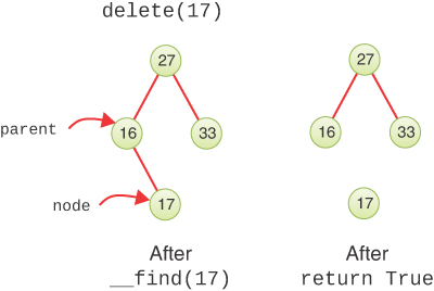
FIGURE 8-18 Deleting a node with no children
If you’re using a language like Python or Java that has garbage collection, the deleted node’s memory will eventually be reclaimed for other uses (if you eliminate all references to it in the program). In languages that require explicit allocation and deallocation of memory, the deleted node should be released for reuse.
Using the Visualization Tool to Delete a Node with No Children
Try deleting a leaf node using the Binary Search Tree Visualization tool. You can either type the key of a node in the text entry box or select a leaf with your pointer device and then select Delete. You see the program use __find() to locate the node by its key, copy it to a temporary variable, set the parent link to None, and then “return” the deleted key and data (in the form of its colored background).
Case 2: The Node to Be Deleted Has One Child
This second case isn’t very difficult either. The node has only two edges: one to its parent and one to its only child. You want to “cut” the node out of this sequence by connecting its parent directly to its child. This process involves changing the appropriate reference in the parent (leftChild or rightChild or __root) to point to the deleted node’s child. Figure 8-19 shows the deletion of node 16, which has only one child.

FIGURE 8-19 Deleting a node with one child
After finding the node and its parent, the delete method has to change only one reference. The deleted node, key 16 in the figure, becomes disconnected from the tree (although it may still have a child pointer to the node that was promoted up (key 20). Garbage collectors are sophisticated enough to know that they can reclaim the deleted node without following its links to other nodes that might still be needed.
Now let’s go back to the case of deleting a node with no children. In that case, the delete method also made a single change to replace one of the parent’s child pointers. That pointer was set to None because there was no replacement child node. That’s a similar operation to Case 2, so you can treat Case 1 and Case 2 together by saying, “If the node to be deleted, D, has 0 or 1 children, replace the appropriate link in its parent with either the left child of D, if it isn’t empty, or the right child of D.” If both child links from D are None, then you’ve covered Case 1. If only one of D’s child links is non-None, then the appropriate child will be selected as the parent’s new child, covering Case 2. You promote either the single child or None into the parent’s child (or possibly __root) reference.
Using the Visualization Tool to Delete a Node with One Child
Let’s assume you’re using the Visualization tool on the tree in Figure 8-5 and deleting node 61, which has a right child but no left child. Click node 61 and the key should appear in the text entry area, enabling the Delete button. Selecting the button starts another call to __find() that stops with current pointing to the node and parent pointing to node 59.
After making a copy of node 61, the animation shows the right child link from node 59 being set to node 61’s right child, node 62. The original copy of node 61 goes away, and the tree is adjusted to put the subtree rooted at node 62 into its new position. Finally, the copy of node 61 is moved to the output box at the bottom.
Use the Visualization tool to generate new trees with single child nodes and see what happens when you delete them. Look for the subtree whose root is the deleted node’s child. No matter how complicated this subtree is, it’s simply moved up and plugged in as the new child of the deleted node’s parent.
Python Code to Delete a Node
Let’s now look at the code for at least Cases 1 and 2. Listing 8-8 shows the code for the delete() method, which takes one argument, the key of the node to delete. It returns either the data of the node that was deleted or None, to indicate the node was not found. That makes it behave somewhat like the methods for popping an item off a stack or deleting an item from a queue. The difference is that the node must be found inside the tree instead of being at a known position in the data structure.
LISTING 8-8 The delete() Method of BinarySearchTree

class BinarySearchTree(object):             # A binary search tree class
…
   def delete(self, goal):                  # Delete a node whose key matches goal
      node, parent = self.__find(goal) # Find goal and its parent
      if node is not None:                  # If node was found,
         return self.__delete(              # then perform deletion at node
            parent, node)                   # under the parent

   def __delete(self,                       # Delete the specified node in the tree
                parent, node):              # modifying the parent node/tree
      deleted = node.data                   # Save the data that's to be deleted
      if node.leftChild:                    # Determine number of subtrees
         if node.rightChild:                # If both subtrees exist,
            self.__promote_successor(       # Then promote successor to
               node)                        # replace deleted node
         else:                              # If no right child, move left child up
            if parent is self:              # If parent is the whole tree,
               self.__root = node.leftChild # update root
            elif parent.leftChild is node:  # If node is parent's left,
               parent.leftChild = node.leftChild # child, update left
            else:                           # else update right child
               parent.rightChild = node.leftChild
      else:                                 # No left child; so promote right child
         if parent is self:                 # If parent is the whole tree,
            self.__root = node.rightChild   # update root
         elif parent.leftChild is node:     # If node is parent's left
            parent.leftChild = node.rightChild # child, then update
         else:                              # left child link else update
            parent.rightChild = node.rightChild # right child
      return deleted                        # Return the deleted node's data
Just like for insertion, the first step is to find the node to delete and its parent. If that search does not find the goal node, then there’s nothing to delete from the tree, and delete() returns None. If the node to delete is found, the node and its parent are passed to the private __delete() method to modify the nodes in the tree.
Inside the __delete() method, the first step is to store a reference to the node data being deleted. This step enables retrieval of the node’s data after the references to it are removed from the tree. The next step checks how many subtrees the node has. That determines what case is being processed. If both a left and a right child are present, that’s Case 3, and it hands off the deletion to another private method, __promote_successor(), which we describe a little later.
If there is only a left subtree of the node to delete, then the next thing to look at is its parent node. If the parent is the BinarySearchTree object (self), then the node to delete must be the root node, so the left child is promoted into the root node slot. If the parent’s left child is the node to delete, then the parent’s left child link is replaced with the node’s left child to remove the node. Otherwise, the parent’s right child link is updated to remove the node.
Notice that working with references makes it easy to move an entire subtree. When the parent’s reference to the node is updated, the child that gets promoted could be a single node or an immense subtree. Only one reference needs to change. Although there may be lots of nodes in the subtree, you don’t need to worry about moving them individually. In fact, they “move” only in the sense of being conceptually in different positions relative to the other nodes. As far as the program is concerned, only the parent’s reference to the root of the subtree has changed, and the rest of the contents in memory remain the same.
The final else clause of the __delete() method deals with the case when the node has no left child. Whether or not the node has a right child, __delete() only needs to update the parent’s reference to point at the node’s right child. That handles both Case 1 and Case 2. It still must determine which field of the parent object gets the reference to the node’s right child, just as in the earlier lines when only the left child was present. It puts the node.rightChild in either the __root, leftChild, or rightChild field of the parent, accordingly. Finally, it returns the data of the node that was deleted.
Case 3: The Node to Be Deleted Has Two Children
Now the fun begins. If the deleted node has two children, you can’t just replace it with one of these children, at least if the child has its own (grand) children. Why not? Examine Figure 8-20 and imagine deleting node 27 and replacing it with its right subtree, whose root is 33. You are promoting the right subtree, but it has its own children. Which left child would node 33 have in its new position, the deleted node’s left child, 16, or node 33’s left child, 28? And what do you do with the other left child? You can’t just throw it away.

FIGURE 8-20 Options for deleting a node with two subtrees
The middle option in Figure 8-20 shows potentially allowing three children. That would bring a whole host of other problems because the tree is no longer binary (see Chapter 9 for more on that idea). The right-hand option in the figure shows pushing the deleted node’s left child, 16, down and splicing in the new node’s left child, 28, above it. That approach looks plausible. The tree is still a binary search tree, at least. The problem, however, is what to do if the promoted node’s left child has a complicated subtree of its own (for example, if node 28 in the figure had a whole subtree below it). That could mean following a long path to figure out where to splice the left subtrees together.
We need another approach. The good news is that there’s a trick. The bad news is that, even with the trick, there are special cases to consider. Remember that, in a binary search tree, the nodes are arranged in order of ascending keys. For each node, the node with the next-highest key is called its in-order successor, or simply its successor. In the original tree of Figure 8-20, node 28 is the in-order successor of node 27.
Here’s the trick: To delete a node with two children, replace the node with its in-order successor. Figure 8-21 shows a deleted node being replaced by its successor. Notice that the nodes are still in order. All it took was a simple replacement. It’s going to be a little more complicated if the successor itself has children; we look at that possibility in a moment.
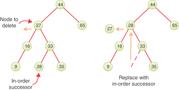
FIGURE 8-21 Node replaced by its successor
Finding the Successor
How do you find the successor of a node? Human beings can do this quickly (for small trees, anyway). Just take a quick glance at the tree and find the next-largest number following the key of the node to be deleted. In Figure 8-21 it doesn’t take long to see that the successor of 27 is 28, or that the successor of 35 is 44. The computer, however, can’t do things “at a glance"; it needs an algorithm.
Remember finding the node with the minimum or maximum key? In this case you’re looking for the minimum key larger than the key to be deleted. The node to be deleted has both a left and right subtree because you’re working on Case 3. So, you can just look for the minimum key in the right subtree, as illustrated in Figure 8-22. All you need to do is follow the left child links until you find a node with no left child.
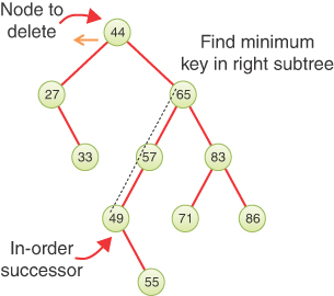
FIGURE 8-22 Finding the successor
What about potential nodes in the trees rooted above the node to be deleted? Couldn’t the successor be somewhere in there? Let’s think it through. Imagine you seek the successor of node 27 in Figure 8-22. The successor would have to be greater than 27 and less than 33, the key of its right child. Any node with a key between those two values would be inserted somewhere in the left subtree of node 33. Remember that you always search down the binary search tree choosing the path based on the key’s relative order to the keys already in the tree. Furthermore, node 33 was placed as the right child of node 27 because it was less than the root node, 44. Any node’s right child key must be less than its parent’s key if it is the left child of that parent. So going up to parent, grandparent, or beyond (following left child links) only leads to larger keys, and those keys can’t be the successor.
There are a couple of other things to note about the successor. If the right child of the original node to delete has no left children, this right child is itself the successor, as shown in the example of Figure 8-23. Because the successor always has an empty left child link, it has at most one child.

FIGURE 8-23 The right child is the successor
Replacing with the Successor
Having found the successor, you can easily copy its key and data values into the node to be deleted, but what do you do with the subtree rooted at the successor node? You can’t leave a copy of the successor node in the tree there because the data would be stored in two places, create duplicate keys, and make deleting the successor a problem in the future. So, what’s the easiest way to get it out of the tree?
Hopefully, reading Chapter 6 makes the answer jump right out. You can now delete the successor from the tree using a recursive call. You want to do the same operation on the successor that you’ve been doing on the original node to delete—the one with the goal key. What’s different is that you only need to do the deletion in a smaller tree, the right subtree where you found the successor. If you tried to do it starting from the root of the tree after replacing the goal node, the __find() method would follow the same path and end at the node you just replaced. You could get around that problem by delaying the replacement of the key until after deleting the successor, but it’s much easier—and more importantly, faster—if you start a new delete operation in the right subtree. There will be much less tree to search, and you can’t accidentally end up at the previous goal node.
In fact, when you searched for the successor, you followed child links to determine the path, and that gave you both the successor and the successor’s parent node. With those two references available, you now have everything needed to call the private __delete() method shown in Listing 8-8. You can now define the __promote_successor() method, as shown in Listing 8-9. Remember, this is the method used to handle Case 3—when the node to delete has two children.
The __promote_successor() method takes as its lone parameter the node to delete. Because it is going to replace that node’s data and key and then delete the successor, it’s easier to refer to it as the node to be replaced in this context. To start, it points a successor variable at the right child of the node to be replaced. Just like the __find() method, it tracks the parent of the successor node, which is initialized to be the node to be replaced. Then it acts like the minNode() method, using a while loop to update successor with its left child if there is a left child. When the loop exits, successor points at the successor node and parent to its parent node.
LISTING 8-9 The __promote_successor() Method of BinarySearchTree

class BinarySearchTree(object):        # A binary search tree class
…
   def __promote_successor(            # When deleting a node with both subtrees,
         self,                         # find successor on the right subtree, put
                                       # its data in this node, and delete the
         node):                        # successor from the right subtree
      successor = node.rightChild      # Start search for successor in
      parent = node                    # right subtree and track its parent
      while successor.leftChild:         # Descend left child links until
         parent = successor            # no more left links, tracking parent
         successor = successor.leftChild
      node.key = successor.key         # Replace node to delete with
      node.data = successor.data       # successor's key and data
      self.__delete(parent, successor) # Remove successor node
All that’s left to do is update the key and data of the node to be replaced and delete the successor node using a recursive call to __delete(). Unlike previous recursive methods you’ve seen, this isn’t a call to the same routine where the call occurs. In this case, the __promote_successor() method calls __delete(), which in turn, could call __promote_successor(). This is called mutual recursion—where two or more routines call each other.
Your senses should be tingling now. How do you know this mutual recursion will end? Where’s the base case that you saw with the “simple” recursion routines? Could you get into an infinite loop of mutually recursive calls? That’s a good thing to worry about, but it’s not going to happen here. Remember that deleting a node broke down into three cases. Cases 1 and 2 were for deleting leaf nodes and nodes with one child. Those two cases did not lead to __promote_successor() calls, so they are the base cases. When you do call __promote_successor() for Case 3, it operates on the subtree rooted at the node to delete, so the only chance that the tree being processed recursively isn’t smaller than the original is if the node to delete is the root node. The clincher, however, is that __promote_successor() calls __delete() only on successor nodes—nodes that are guaranteed to have at most one child and at least one level lower in the tree than the node they started on. Those always lead to a base case and never to infinite recursion.
Using the Visualization Tool to Delete a Node with Two Children
Generate a tree with the Visualization tool and pick a node with two children. Now mentally figure out which node is its successor, by going to its right child and then following down the line of this right child’s left children (if it has any). For your first try, you may want to make sure the successor has no children of its own. On later attempts, try looking at the more complicated situation where entire subtrees of the successor are moved around, rather than a single node.
After you’ve chosen a node to delete, click the Delete button. You may want to use the Step or Pause/Play buttons to track the individual steps. Each of the methods we’ve described will appear in the code window, so you can see how it decides the node to delete has two children, locates the successor, copies the successor key and data, and then deletes the successor node.
Is Deletion Necessary?
If you’ve come this far, you can see that deletion is fairly involved. In fact, it’s so complicated that some programmers try to sidestep it altogether. They add a new Boolean field to the __Node class, called something like isDeleted. To delete a node, they simply set this field to True. This is a sort of a “soft” delete, like moving a file to a trash folder without truly deleting it. Then other operations, like __find(), check this field to be sure the node isn’t marked as deleted before working with it. This way, deleting a node doesn’t change the structure of the tree. Of course, it also means that memory can fill up with previously “deleted” nodes.
This approach is a bit of a cop-out, but it may be appropriate where there won’t be many deletions in a tree. Be very careful. Assumptions like that tend to come back to haunt you. For example, assuming that deletions might not be frequent for a company’s personnel records might encourage a programmer to use the isDeleted field. If the company ends up lasting for hundreds of years, there are likely to be more deletions than active employees at some point in the future. The same is true if the company experiences high turnover rates, even over a short time frame. That will significantly affect the performance of the tree operations.
The Efficiency of Binary Search Trees
As you’ve seen, most operations with trees involve descending the tree from level to level to find a particular node. How long does this operation take? We mentioned earlier that the efficiency of finding a node could range from O(log N) to O(N), but let’s look at the details.
In a full, balanced tree, about half the nodes are on the bottom level. More accurately, in a full, balanced tree, there’s exactly one more node on the bottom row than in the rest of the tree. Thus, about half of all searches or insertions or deletions require finding a node on the lowest level. (About a quarter of all search operations require finding the node on the next-to-lowest level, and so on.)
During a search, you need to visit one node on each level. You can get a good idea how long it takes to carry out these operations by knowing how many levels there are. Assuming a full, balanced tree, Table 8-1 shows how many levels are necessary to hold a given number of nodes.
Table 8-1 Number of Levels for Specified Number of Nodes
Number of Nodes | Number of Levels |
|---|---|
1 | 1 |
3 | 2 |
7 | 3 |
15 | 4 |
31 | 5 |
… | … |
1,023 | 10 |
… | … |
32,767 | 15 |
… | … |
1,048,575 | 20 |
… | … |
33,554,431 | 25 |
… | … |
1,073,741,823 | 30 |
The numbers are very much like those for searching the ordered array discussed in Chapter 2. In that case, the number of comparisons for a binary search was approximately equal to the base 2 logarithm of the number of cells in the array. Here, if you call the number of nodes in the first column N, and the number of levels in the second column L, you can say that N is 1 less than 2 raised to the power L, or
N = 2L – 1
Adding 1 to both sides of the equation, you have
N + 1 = 2L
Using what you learned in Chapter 2 about logarithms being the inverse of raising a number to a power, you can take the logarithm of both sides and rearrange the terms to get
log2(N + 1) = log2(2L) = L
L = log2(N + 1)
Thus, the time needed to carry out the common tree operations is proportional to the base 2 log of N. In Big O notation, you say such operations take O(log N) time.
If the tree isn’t full or balanced, the analysis is difficult. You can say that for a tree with a given number of levels, average search times will be shorter for the nonfull tree than the full tree because fewer searches will proceed to lower levels.
Compare the tree to the other data storage structures we’ve discussed so far. In an unordered array or a linked list containing 1,000,000 items, finding the item you want takes, on average, 500,000 comparisons, basically O(N). In a balanced tree of 1,000,000 items, only 20 (or fewer) comparisons are required because it’s O(log N).
In an ordered array, you can find an item equally quickly, but inserting an item requires, on average, moving 500,000 items. Inserting an item in a tree with 1,000,000 items requires 20 or fewer comparisons, plus a small amount of time to connect the item. The extra time is constant and doesn’t depend on the number of items.
Similarly, deleting an item from a 1,000,000-item array requires moving an average of 500,000 items, while deleting an item from a 1,000,000-node tree requires 20 or fewer comparisons to find the item, plus a few more comparisons to find its successor, plus a short time to disconnect the item and connect its successor. Because the successor is somewhere lower in the tree than the node to delete, the total number of comparisons to find both the node and its successor will be 20 or fewer.
Thus, a tree provides high efficiency for all the common data storage operations: searches, insertions, and deletions. Traversing is not as fast as the other operations, but it must be O(N) to cover all N items, by definition. In all the data structures you’ve seen, it has been O(N), but we show some other data structures later where it could be greater. There is a little more memory needed for traversing a tree compared to arrays or lists because you need to store the recursive calls or use a stack. That memory will be O(log N). That contrasts with the arrays and lists that need only O(1) memory during traversal.
Trees Represented as Arrays
Up to now, we’ve represented the binary tree nodes using objects with references for the left and right children. There’s a completely different way to represent a tree: with an array.
In the array approach, the nodes are stored in an array and are not linked by references. The position of the node in the array corresponds to its position in the tree. We put the root node at index 0. The root’s left child is placed at index 1, and its right child at index 2, and so on, progressing from left to right along each level of the tree. This approach is shown in Figure 8-24, which is a binary search tree with letters for the keys.
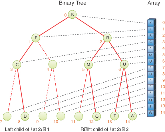
FIGURE 8-24 A binary tree represented by an array
Every position in the tree, whether it represents an existing node or not, corresponds to a cell in the array. Adding a node at a given position in the tree means inserting the node into the equivalent cell in the array. Cells representing tree positions with no nodes are filled with 0, None, or some other special value that cannot be confused with a node. In the figure, the ° symbol is used in the array for empty nodes.
With this scheme, a node’s children and parent can be found by applying some simple arithmetic to the node’s index number in the array. If a node’s index number is index, this node’s left child is
2 * index + 1
its right child is
2 * index + 2
and its parent is
(index – 1) // 2
(where the // indicates integer division with no remainder). You can verify these formulas work by looking at the indices in Figure 8-24. Any algorithm that follows links between nodes can easily determine where to check for the next node. The scheme works for any binary tree, not just binary search trees. It has the nice feature that edges/links between nodes are just as easy to travel up as they are going down (without the double linking needed for lists). Even better, it can be generalized to any tree with a fixed number of children.
In most situations, however, representing a tree with an array isn’t very efficient. Unfilled nodes leave holes in the array, wasting memory. Even worse, when deletion of a node involves moving subtrees, every node in the subtree must be moved to its new location in the array, which is time-consuming in large trees. For insertions that insert nodes beyond the current maximum depth of the tree, the array may need to be resized.
If deletions aren’t allowed or are very rare and the maximum depth of the tree can be predicted, the array representation may be useful, especially if obtaining memory for each node dynamically is, for some reason, too time-consuming. That might be the case when programming in assembly language or a very limited operating system, or a system with no garbage collection.
Tree Levels and Size
When trees are represented as arrays, the maximum level and number of nodes is constrained by the size of the array. For linked trees, there’s no specific maximum. For both representations, the current maximum level and number of nodes can be determined only by traversing the tree. If there will be frequent calls to request these metrics, the BinarySearchTree object can maintain values for them, but the insert() and delete() methods must be modified to update the values as nodes are added and removed.
To count nodes in a linked tree, you can use the traverse() method to iterate over all the nodes and increment a count, as shown earlier in the example to find the average key value and again in the nodes() method of Listing 8-10. To find the maximum level, you cannot use the same technique because the level of each node during the traversal is not provided (although it could be added by modifying the generator). Instead, the recursive definition shown in Listing 8-10 gets the job done in a few lines of code.
LISTING 8-10 The levels() and nodes() Methods of BinarySearchTree
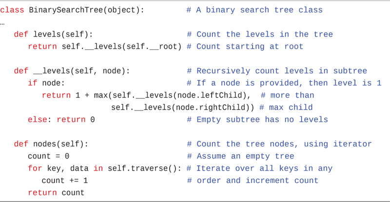
class BinarySearchTree(object):         # A binary search tree class
…
   def levels(self):                    # Count the levels in the tree
      return self.__levels(self.__root) # Count starting at root

   def __levels(self, node):            # Recursively count levels in subtree
      if node:                          # If a node is provided, then level is 1
         return 1 + max(self.__levels(node.leftChild),  # more than
                        self.__levels(node.rightChild)) # max child
      else: return 0                    # Empty subtree has no levels

   def nodes(self):                     # Count the tree nodes, using iterator
      count = 0                         # Assume an empty tree
      for key, data in self.traverse(): # Iterate over all keys in any
         count += 1                     # order and increment count
      return count
Counting the levels of a subtree is somewhat different than what you’ve seen before in that each node takes the maximum level of each of its subtrees and adds one to it for the node itself. It might seem as if there should be a shortcut by looking at the depth of the minimum or maximum key so that you don’t need to visit every node. If you think about it, however, even finding the minimum and maximum keys shows the depth only on the left and right “flanks” of the tree. There could be longer paths somewhere in the middle, and the only way to find them is to visit all the nodes.
Printing Trees
You’ve seen how to traverse trees in different orders. You could always use the traversal method to print all the nodes in the tree, as shown in the Visualization tool. Using the in-order traversal would show the items in increasing order of their keys. On a two-dimensional output, you could use the in-order sequence to position the nodes along the horizontal axis and the level of each node to determine its vertical position. That could produce tree diagrams like the ones shown in the previous figures.
On a simple command-line output, it’s easier to print one node per line. The problem then becomes positioning the node on the line to indicate the shape of the tree. If you want the root node at the top, then you must compute the width of the full tree and place that node in the middle of the full width. More accurately, you would have to compute the width of the left and right subtrees and use that to position the root in order to show balanced and unbalanced trees accurately.
On the other hand, if you place the root at the left side of an output line and show the level of nodes as indentation from the leftmost column, it’s easy to print the tree on a terminal. Doing so essentially rotates the tree 90° to the left. Each node of the tree appears on its own line of the output. That allows you to forget about determining the width of subtrees and write a simple recursive method, as shown in Listing 8-11.
LISTING 8-11 Methods to Print Trees with One Node per Line
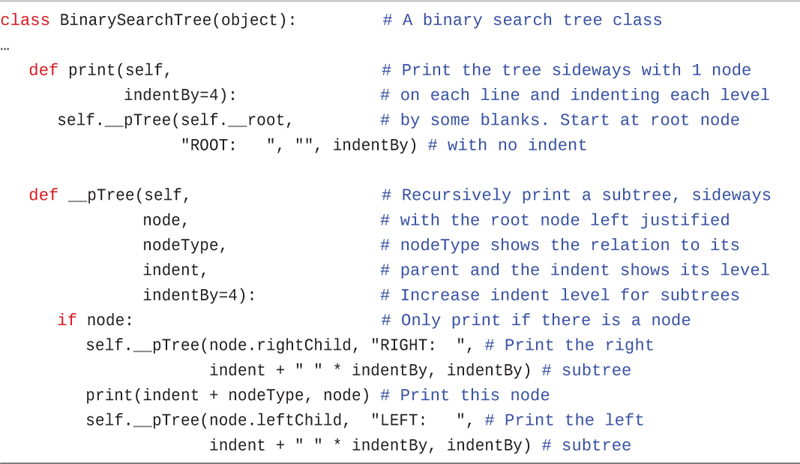
class BinarySearchTree(object):         # A binary search tree class
…
   def print(self,                      # Print the tree sideways with 1 node
             indentBy=4):               # on each line and indenting each level
      self.__pTree(self.__root,         # by some blanks. Start at root node
                   "ROOT:   ", "", indentBy) # with no indent

   def __pTree(self,                    # Recursively print a subtree, sideways
               node,                    # with the root node left justified
               nodeType,                # nodeType shows the relation to its
               indent,                  # parent and the indent shows its level
               indentBy=4):             # Increase indent level for subtrees
      if node:                          # Only print if there is a node
         self.__pTree(node.rightChild, "RIGHT:  ", # Print the right
                      indent + " " * indentBy, indentBy) # subtree
         print(indent + nodeType, node) # Print this node
         self.__pTree(node.leftChild,  "LEFT:   ", # Print the left
                      indent + " " * indentBy, indentBy) # subtree
The public print() method calls the private __pTree() method to recursively print the nodes starting at the root node. It takes a parameter, indentBy, to control how many spaces are used to indent each level of the tree. It labels the nodes to show their relationship with their parent (if it wasn’t already clear from their indentation and relative positions). The recursive method implementation starts by checking the base case, an empty node, in which case nothing needs to be printed. For every other node, it first recursively prints the right subtree because that is the top of the printed version. It adds spaces to the indent so that subtree is printed further to the right. Then it prints the current node prefixed with its indentation and nodeType label. Lastly, it prints the left subtree recursively with the extended indentation. This produces an output such as that shown in Figure 8-25. The nodes are printed as {key, data} pairs and the figure example has no data stored with it.
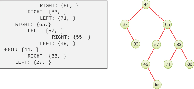
FIGURE 8-25 Tree printed with indentation for node depth
In printing the tree like this, you use a different traversal order from the three standard ones. The print order uses a reverse in-order traversal of the tree.
Duplicate Keys
As in other data structures, the problem of duplicate keys must be addressed. In the code shown for insert() and in the Visualization tool, a node with a duplicate key will not be inserted. The tool shows the data for the node being updated by moving a new colored circle to fill the node.
To allow for duplicate keys, you must make several choices. The duplicates go in the right subtree based on the fundamental binary search tree rule. They form a chain of nodes with only right child links, as shown in Figure 8-26. One of the design choices is where to put any left child link. It should go only at the first or last duplicate in the chain so that the algorithms know where to find it. The figure illustrates the two choices. New duplicate keys should be inserted at the opposite end of the chain.

FIGURE 8-26 Duplicate keys in binary search trees
Another choice is what to return from the __find() and search() methods for a key that has duplicates. Should it return the first or the last? The choice should also be consistent with what node is deleted and returned by the delete() method. If they are inserted at the first and removed from the first, then delete() will act like a mini stack for the duplicate nodes.
The delete operation is complicated by the fact that different data values could be stored at each of the duplicate nodes. The caller may need to delete a node with specific data, rather than just any node with the duplicate key. Whichever scheme is selected, the deletion routine will need to ensure that the left subtree, if any, remains attached to the appropriate place.
With any kind of duplicate keys, balancing the tree becomes difficult or impossible. The chains of duplicates add extra levels that cannot be rearranged to help with balance. That means the efficiency of finding an item moves away from best case of O(log N) toward O(N).
As you can see, allowing duplicate keys is not a simple enhancement to the data structure. In other data structures, duplicate keys present challenges, but not all of them are as tricky as the binary search tree.
The BinarySearchTreeTester.py Program
It’s always a good idea to test the functioning of a code module by writing tests that exercise each operation. Writing a comprehensive set of tests is an art in itself. Another useful strategy is to write an interactive test program that allows you to try a series of operations in different orders and with different arguments. To test all the BinarySearchTree class methods shown, you can use a program like BinarySearchTreeTester.py shown in Listing 8-12.
LISTING 8-12 The BinarySearchTreeTester.py Program
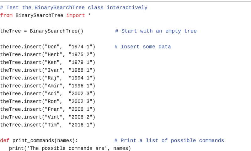
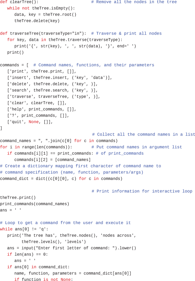
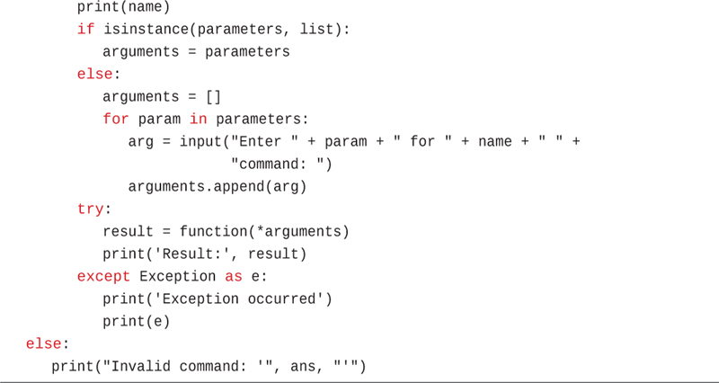
# Test the BinarySearchTree class interactively
from BinarySearchTree import *

theTree = BinarySearchTree()          # Start with an empty tree

theTree.insert("Don",  "1974 1")      # Insert some data
theTree.insert("Herb", "1975 2")
theTree.insert("Ken",  "1979 1")
theTree.insert("Ivan", "1988 1")
theTree.insert("Raj",  "1994 1")
theTree.insert("Amir", "1996 1")
theTree.insert("Adi",  "2002 3")
theTree.insert("Ron",  "2002 3")
theTree.insert("Fran", "2006 1")
theTree.insert("Vint", "2006 2")
theTree.insert("Tim",  "2016 1")

def print_commands(names):            # Print a list of possible commands
   print('The possible commands are', names)

def clearTree():                      # Remove all the nodes in the tree
   while not theTree.isEmpty():
      data, key = theTree.root()
      theTree.delete(key)

def traverseTree(traverseType="in"):  # Traverse & print all nodes
   for key, data in theTree.traverse(traverseType):
      print('{', str(key), ', ', str(data), '}', end=' ')
   print()

commands = [  # Command names, functions, and their parameters
   ['print', theTree.print, []],
   ['insert', theTree.insert, ('key', 'data')],
   ['delete', theTree.delete, ('key', )],
   ['search', theTree.search, ('key', )],
   ['traverse', traverseTree, ('type', )],
   ['clear', clearTree, []],
   ['help', print_commands, []],
   ['?', print_commands, []],
   ['quit', None, []],
]
                                      # Collect all the command names in a list
command_names = ", ".join(c[0] for c in commands)
for i in range(len(commands)):        # Put command names in argument list
   if commands[i][1] == print_commands: # of print_commands
      commands[i][2] = [command_names]
# Create a dictionary mapping first character of command name to
# command specification (name, function, parameters/args)
command_dict = dict((c[0][0], c) for c in commands)

                                      # Print information for interactive loop
theTree.print()
print_commands(command_names)
ans = ' '

# Loop to get a command from the user and execute it
while ans[0] != 'q':
   print('The tree has', theTree.nodes(), 'nodes across',
         theTree.levels(), 'levels')
   ans = input("Enter first letter of command: ").lower()
   if len(ans) == 0:
      ans = ' '
   if ans[0] in command_dict:
      name, function, parameters = command_dict[ans[0]]
      if function is not None:
         print(name)
         if isinstance(parameters, list):
            arguments = parameters
         else:
            arguments = []
            for param in parameters:
               arg = input("Enter " + param + " for " + name + " " +
                           "command: ")
               arguments.append(arg)
         try:
            result = function(*arguments)
            print('Result:', result)
         except Exception as e:
            print('Exception occurred')
            print(e)
   else:
      print("Invalid command: '", ans, "'")
This program allows users to enter commands by typing them in a terminal interface. It first imports the BinarySearchTree module and creates an empty tree with it. Then it puts some data to it, using insert() to associate names with some strings. The names are the keys used to place the nodes within the tree.
The tester defines several utility functions to print all the possible commands, clear all the nodes from the tree, and traverse the tree to print each node. These functions handle commands in the command loop below.
The next part of the tester program defines a list of commands. For each one, it has a name, a function to execute the command, and a list or tuple of arguments or parameters. This is more advanced Python code than we’ve shown so far, so it might look a little strange. The names are what the user will type (or at least their first letter), and the functions are either methods of the tree or the utility functions defined in the tester. The arguments and parameters will be processed after the user chooses a command.
To provide a little command-line help, the tester concatenates the list of command names into a string, separating them with commas. This operation is accomplished with the join() method of strings. The text to place between each command name is the string (a comma and a space), and the argument to join() is the list of names. The program uses a list comprehension to iterate through the command specifications in commands and pull out the first element, which is the command name: ”, ”.join(c[0] for c in commands). The result is stored in the command_names variable.
Then the concatenated string of command names needs to get inserted in the argument list for the print_commands function. That’s done in the for loop. Two entries have the print_commands function: the help and ? commands.
The last bit of preparation for the command loop creates a dictionary, command_dict, that maps the first character of each command to the command specification. You haven’t used this Python data structure yet. In Chapter 11, “Hash Tables,” you see how they work, so if you’re not familiar with them, think of them as an associative array—an array indexed by a string instead of integer. You can assign values in the array and then look them up quickly. In the tester program, evaluating command_dict['p'] would return the specification for the print command, namely ['print', theTree.print, []]. Those specifications get stored in the dictionary using the compact (but cryptic) comprehension: dict((c[0][0], c) for c in commands).
The rest of the tester implements the command loop. It first prints the tree on the terminal, followed by the list of commands. The ans variable holds the input typed by the user. It gets initialized to a space so that the command loop starts and prompts for a new command.
The command loop continues until the user invokes the quit command, which starts with q. Inside the loop body, the number of nodes and levels in the tree is printed, and then the user is asked for a command. The string that is returned by input() is converted to lowercase to simplify the command lookup. If the user just pressed Return, there would be no first character in the string, so you would fill in a ? to make the default response be to print all the command names again.
In the next statement—if ans[0] in command_dict:—the tester checks whether the first character in the user’s response is one of the known commands. If the character is recognized, it extracts the name, function, and parameters from the specification stored in the command_dict. If there’s a function to execute, then it will be processed. If not, then the user asked to quit, and the while loop will exit. When the first character of the user’s response does not match a command, an error message is printed, and the loop prompts for a new command.
After the command specification is found, it either needs to prompt the user for the arguments to use when calling the function or get them from the specification. This choice is based on whether the parameters were specified as Python tuple or list. If it’s a tuple, the elements of the tuple are the names of the parameters. If it’s a list, then the list contains the arguments of the function. For tuples, the user is prompted to enter each argument by name, and the answers are stored in the arguments list. After the arguments are determined, the command loop tries calling the function with the arguments list using result = function(*arguments). The asterisk (*) before the arguments is not a multiplication operator. It means that the arguments list should be used as the list of positional arguments for the function. If the function raises any exceptions, they are caught and displayed. Otherwise, the result of the function is printed before looping to get another command.
Try using the tester to run the four main operations: search, insert, traverse, and delete. For the deletion, try deleting nodes with 0, 1, and 2 child nodes to see the effect. When you delete a node with 2 children, predict which successor node will replace the deleted node and see whether you’re right.
The Huffman Code
You shouldn’t get the idea that binary trees are always search trees. Many binary trees are used in other ways. Figure 8-16 shows an example where a binary tree represents an algebraic expression. We now discuss an algorithm that uses a binary tree in a surprising way to compress data. It’s called the Huffman code, after David Huffman, who discovered it in 1952. Data compression is important in many situations. An example is sending data over the Internet or via digital broadcasts, where it’s important to send the information in its shortest form. Compressing the data means more data can be sent in the same time under the bandwidth limits.
Character Codes
Each character in an uncompressed text file is represented in the computer by one to four bytes, depending on the way characters are encoded. For the venerable ASCII code, only one byte is used, but that limits the range of characters that can be expressed to fewer than 128. To account for all the world’s languages plus other symbols like emojis ![]() , the various Unicode standards use up to four bytes per character. For this discussion, we assume that only the ASCII characters are needed, and each character takes one byte (or eight bits). Table 8-2 shows how some characters are represented in binary using the ASCII code.
, the various Unicode standards use up to four bytes per character. For this discussion, we assume that only the ASCII characters are needed, and each character takes one byte (or eight bits). Table 8-2 shows how some characters are represented in binary using the ASCII code.
Table 8-2 Some ASCII Codes
Character | Decimal | Binary |
|---|---|---|
@ | 64 | 01000000 |
A | 65 | 01000001 |
B | 66 | 01000010 |
… | … | … |
Y | 89 | 01011001 |
Z | 90 | 01011010 |
… | … | … |
a | 97 | 01100001 |
b | 98 | 01100010 |
There are several approaches to compressing data. For text, the most common approach is to reduce the number of bits that represent the most-used characters. As a consequence, each character takes a variable number of bits in the “stream” of bits that represents the full text.
In English, E and T are very common letters, when examining prose and other person-to-person communication and ignoring things like spaces and punctuation. If you choose a scheme that uses only a few bits to write E, T, and other common letters, it should be more compact than if you use the same number of bits for every letter. On the other end of the spectrum, Q and Z seldom appear, so using a large number of bits occasionally for those letters is not so bad.
Suppose you use just two bits for E—say 01. You can’t encode every letter of the English alphabet in two bits because there are only four 2-bit combinations: 00, 01, 10, and 11. Can you use these four combinations for the four most-used characters? Well, if you did, and you still wanted to have some encoding for the lesser-used characters, you would have trouble. The algorithm that interprets the bits would have to somehow guess whether a pair of bits is a single character or part of some longer character code.
One of the key ideas in encoding is that we must set aside some of the code values as indicators that a longer bit string follows to encode a lesser-used character. The algorithm needs a way to look at a bit string of a particular length and determine if that is the full code for one of the characters or just a prefix for a longer code value. You must be careful that no character is represented by the same bit combination that appears at the beginning of a longer code used for some other character. For example, if E is 01, and Z is 01011000, then an algorithm decoding 01011000 wouldn’t know whether the initial 01 represented an E or the beginning of a Z. This leads to a rule: No code can be the prefix of any other code.
Consider also that in some messages, E might not be the most-used character. If the text is a program source file, for example, punctuation characters such as the colon (:), semicolon (;), and underscore (_) might appear more often than E does. Here’s a solution to that problem: for each message, you make up a new code tailored to that particular message. Suppose you want to send the message SPAM SPAM SPAM EGG + SPAM. The letter S appears a lot, and so does the space character. You might want to make up a table showing how many times each letter appears. This is called a frequency table, as shown in Table 8-3.
Table 8-3 Frequency Table for the SPAM Message
Character | Count |
| Character | Count |
|---|---|---|---|---|
A | 4 |
| P | 4 |
E | 1 |
| S | 4 |
G | 2 |
| Space | 5 |
M | 4 |
| + | 1 |
The characters with the highest counts should be coded with a small number of bits. Table 8-4 shows one way how you might encode the characters in the SPAM message.
Table 8-4 Huffman Code for the SPAM Message
Character | Count | Code |
| Character | Count | Code |
|---|---|---|---|---|---|---|
A | 4 | 111 |
| P | 4 | 110 |
E | 1 | 10000 |
| S | 4 | 101 |
G | 2 | 1001 |
| Space | 5 | 01 |
M | 4 | 00 |
| + | 1 | 10001 |
You can use 01 for the space because it is the most frequent. The next most frequent characters are S, P, A, and M, each one appearing four times. You use the code 00 for the last one, M. The remaining codes can’t start with 00 or 01 because that would break the rule that no code can be a prefix of another code. That leaves 10 and 11 to use as prefixes for the other characters.
What about 3-bit code combinations? There are eight possibilities: 000, 001, 010, 011, 100, 101, 110, and 111, but you already know you can’t use anything starting with 00 or 01. That eliminates four possibilities. You can assign some of those 3-bit codes to the next most frequent characters, S as 101, P as 110, and A as 111. That leaves the prefix 100 to use for the remaining characters. You use a 4-bit code, 1001, for the next most frequent character, G, which appears twice. There are two characters that appear only once, E and +. They are encoded with 5-bit codes, 10000 and 10001.
Thus, the entire message is coded as
101 110 111 00 01 101 110 111 00 01 101 110 111 00 01 10000 1001 1001 01 10001 01
101 110 111 00
For legibility, we show this message broken into the codes for individual characters. Of course, all the bits would run together because there is no space character in a binary message, only 0s and 1s. That makes it more challenging to find which bits correspond to a character. The main point, however, is that the 25 characters in the input message, which would typically be stored in 200 bits in memory (8 × 25), require only 72 bits in the Huffman coding.
Decoding with the Huffman Tree
We show later how to create Huffman codes. First, let’s examine the somewhat easier process of decoding. Suppose you received the string of bits shown in the preceding section. How would you transform it back into characters? You could use a kind of binary tree called a Huffman tree. Figure 8-27 shows the Huffman tree for the SPAM message just discussed.

FIGURE 8-27 Huffman tree for the SPAM message
The characters in the message appear in the tree as leaf nodes. The higher their frequency in the message, the higher up they appear in the tree. The number outside each leaf node is its frequency. That puts the space character (sp) at the second level, and the S, P, A, and M characters at the second or third level. The least frequent, E and +, are on the lowest level, 5.
How do you use this tree to decode the message? You start by looking at the first bit of the message and set a pointer to the root node of the tree. If you see a 0 bit, you move the pointer to the left child of the node, and if you see a 1 bit, you move it right. If the identified node does not have an associated character, then you advance to the next bit in the message. Try it with the code for S, which is 101. You go right, left, then right again, and voila, you find yourself on the S node. This is shown by the blue arrows in Figure 8-27.
You can do the same with the other characters. After you’ve arrived at a leaf node, you can add its character to the decoded string and move the pointer back to the root node. If you have the patience, you can decode the entire bit string this way.
Creating the Huffman Tree
You’ve seen how to use a Huffman tree for decoding, but how do you create this tree? There are many ways to handle this problem. You need a Huffman tree object, and that is somewhat like the BinarySearchTree described previously in that it has nodes that have up to two child nodes. It’s quite different, however, because routines that are specific to keys in search trees, like find(), insert(), and delete(), are not relevant. The constraint that a node’s key be larger than any key of its left child and equal to or less than any key of its right child doesn’t apply to a Huffman tree. Let’s call the new class HuffmanTree, and like the search tree, store a key and a value at each node. The key will hold the decoded message character such as S or G. It could be the space character, as you’ve seen, and it needs a special value for “no character”.
Here is the algorithm for constructing a Huffman tree from a message string:
Preparation
Count how many times each character appears in the message string.
Make a
HuffmanTreeobject for each character used in the message. For the SPAM message example, that would be eight trees. Each tree has a single node whose key is a character and whose value is that character’s frequency in the message. Those values can be found in Table 8-3 or Table 8-4 for the SPAM message.Insert these trees in a priority queue (as described in Chapter 4). They are ordered by the frequency (stored as the value of each root node) and the number of levels in the tree. The tree with the smallest frequency has the highest priority. Among trees with equal frequency, the one with more levels is the highest priority. In other words, when you remove a tree from the priority queue, it’s always the one with the deepest tree of the least-used character. (Breaking ties using the tree depth, improves the balance of the final Huffman tree.)
That completes the preparation, as shown in Step 0 of Figure 8-28. Each single node Huffman trees has a character shown in the center of the node and a frequency value shown below and to the left of the node.
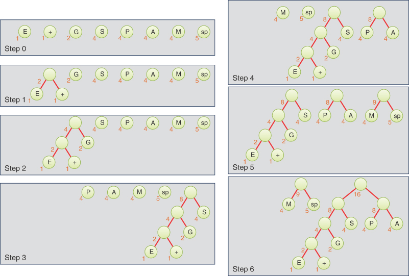
FIGURE 8-28 Growing the Huffman tree, first six steps
Then do the following:
Tree consolidation
Remove two trees from the priority queue and make them into children of a new node. The new node has a frequency value that is the sum of the children’s frequencies; its character key can be left blank (the special value for no character, not the space character).
Insert this new, deeper tree back into the priority queue.
Keep repeating steps 1 and 2. The trees will get larger and larger, and there will be fewer and fewer of them. When there is only one tree left in the priority queue, it is the Huffman tree and you’re done.
Figure 8-28 and Figure 8-29 show how the Huffman tree is constructed for the SPAM message.
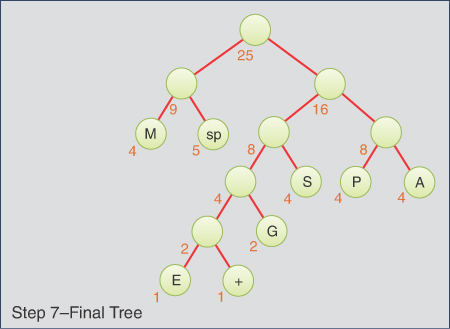
FIGURE 8-29 Growing the Huffman tree, final step
Coding the Message
Now that you have the Huffman tree, how do you encode a message? You start by creating a code table, which lists the Huffman code alongside each character. To simplify the discussion, we continue to assume that only ASCII characters are possible, so we need a table with 128 cells. The index of each cell would be the numerical value of the ASCII character: 65 for A, 66 for B, and so on. The contents of the cell would be the Huffman code for the corresponding character. Initially, you could fill in some special value for indicating “no code” like None or an empty string in Python to check for errors where you failed to make a code for some character.
Such a code table makes it easy to generate the coded message: for each character in the original message, you use its code as an index into the code table. You then repeatedly append the Huffman codes to the end of the coded message until it’s complete.
To fill in the codes in the table, you traverse the Huffman tree, keeping track of the path to each node as it is visited. When you visit a leaf node, you use the key for that node as the index to the table and insert the path as a binary string into the cell’s value. Not every cell contains a code—only those appearing in the message. Figure 8-30 shows how this looks for the SPAM message. The table is abbreviated to show only the significant rows. The path to the leaf node for character G is shown as the tree is being traversed.

FIGURE 8-30 Building the code table
The full code table can be built by calling a method that starts at the root and then calls itself recursively for each child. Eventually, the paths to all the leaf nodes will be explored, and the code table will be complete.
One more thing to consider: if you receive a binary message that’s been compressed with a Huffman code, how do you know what Huffman tree to use for decoding it? The answer is that the Huffman tree must be sent first, before the binary message, in some format that doesn’t require knowledge of the message content. Remember that Huffman codes are for compressing the data, not encrypting it. Sending a short description of the Huffman tree followed by a compressed version of a long message saves many bits.
Summary
- Trees consist of nodes connected by edges.
- The root is the topmost node in a tree; it has no parent.
- All nodes but the root in a tree have exactly one parent.
- In a binary tree, a node has at most two children.
- Leaf nodes in a tree have no child nodes and exactly one path to the root.
- An unbalanced tree is one whose root has many more left descendants than right descendants, or vice versa.
- Each node of a tree stores some data. The data typically has a key value used to identify it.
- Edges are most commonly represented by references to a node’s children; less common are references from a node to its parent.
- Traversing a tree means visiting all its nodes in some predefined order.
- The simplest traversals are pre-order, in-order, and post-order.
- Pre-order and post-order traversals are useful for parsing algebraic expressions.
- Binary Search Trees
- In a binary search tree, all the nodes that are left descendants of node A have key values less than that of A; all the nodes that are A’s right descendants have key values greater than (or equal to) that of A.
- Binary search trees perform searches, insertions, and deletions in O(log N) time.
- Searching for a node in a binary search tree involves comparing the goal key to be found with the key value of a node and going to that node’s left child if the goal key is less or to the node’s right child if the goal key is greater.
- Insertion involves finding the place to insert the new node and then changing a child field in its new parent (or the root of the tree) to refer to it.
- An in-order traversal visits nodes in order of ascending keys.
- When a node has no children, you can delete it by clearing the child field in its parent (for example, setting it to
Nonein Python). - When a node has one child, you can delete it by setting the child field in its parent to point to its child.
- When a node has two children, you can delete it by replacing it with its successor and deleting the successor from the subtree.
- You can find the successor to a node A by finding the minimum node in A’s right subtree.
- Nodes with duplicate key values require extra coding because typically only one of them (the first) is found in a search, and managing their children complicates insertions and deletions.
- Trees can be represented in the computer’s memory as an array, although the reference-based approach is more common and memory efficient.
- A Huffman tree is a binary tree (but not a search tree) used in a data-compression algorithm called Huffman coding.
- In the Huffman code, the characters that appear most frequently are coded with the fewest bits, and those that appear rarely are coded with the most bits.
- The paths in the Huffman tree provide the codes for each of the leaf nodes.
- The level of a leaf node indicates the number of bits used in the code for its key.
- The characters appearing the least frequently in a Huffman coded message are placed in leaf nodes at the deepest levels of the Huffman tree.
Questions
These questions are intended as a self-test for readers. Answers may be found in Appendix C.
1. Insertion and deletion in a binary search tree require what Big O time?
2. A binary tree is a search tree if
a. every nonleaf node has children whose key values are less than or equal to the parent.
b. the key values of every nonleaf node are the sum or concatenation of the keys of its children
c. every left child has a key less than its parent and every right child has a key greater than or equal to its parent.
d. in the path from the root to every leaf node, the key of each node is greater than or equal to the key of its parent.
3. True or False: If you traverse a tree and print the path to each node as a series of the letters L and R for whether the path followed the left or right child at each step, there could be some duplicate paths.
4. When compared to storing data in an ordered array, the main benefit of storing it in a binary search tree is
a. having the same search time as traversal time in Big O notation.
b. not having to copy data when inserting or deleting items.
c. being able to search for an item in O(log N) time.
d. having a key that is separate from the value identified by the key.
5. In a complete, balanced binary tree with 20 nodes, and the root considered to be at level 0, how many nodes are there at level 4?
6. A subtree of a binary tree always has
a. a root that is a child of the main tree’s root.
b. a root unconnected to the main tree’s root.
c. fewer nodes than the main tree.
d. a sibling with an equal or larger number of nodes.
7. When implementing trees as objects, the ______ and the _______ are generally separate classes.
8. Finding a node in a binary search tree involves going from node to node, asking
a. how big the node’s key is in relation to the search key.
b. how big the node’s key is compared to its right or left child’s key.
c. what leaf node you want to reach.
d. whether the level you are on is above or below the search key.
9. An unbalanced tree is one
a. in which most of the keys have values greater than the average.
b. where there are more nodes above the central node than below.
c. where the leaf nodes appear much more frequently as the left child of their parents than as the right child, or vice versa.
d. in which the root or some other node has many more left descendants than right descendants, or vice versa.
10. True or False: A hierarchical file system is essentially a binary search tree, although it can be unbalanced.
11. Inserting a node starts with the same steps as _______ a node.
12. Traversing tree data structures
a. requires multiple methods to handle the different traversal orders.
b. can be implemented using recursive functions or generators.
c. is much faster than traversing array data structures.
d. is a way to make soft deletion of items practical.
13. When a tree is extremely unbalanced, it begins to behave like the ______ data structure.
14. Suppose a node A has a successor node S in a binary search tree with no duplicate keys. Then S must have a key that is larger than _____ but smaller than or equal to _______.
15. Deleting nodes in a binary search tree is complex because
a. copying subtrees below the successor requires another traversal.
b. finding the successor is difficult to do, especially when the tree is unbalanced.
c. the tree can split into multiple trees, a forest, if it’s not done properly.
d. the operation is very different for the different number of child nodes of the node to be deleted, 0, 1, or 2.
16. In a binary tree used to represent a mathematical expression,
a. both children of an operator node must be operands.
b. following a post-order traversal, parentheses must be added.
c. following a pre-order traversal, parentheses must be added.
d. in pre-order traversal, a node is visited before either of its children.
17. When a tree is represented by an array, the right child of a node at index n has an index of _______.
18. True or False: Deleting a node with one child from a binary search tree involves finding that node’s successor.
19. A Huffman tree is typically used to _______ text data.
20. Which of the following is not true about a Huffman tree?
a. The most frequently used characters always appear near the top of the tree.
b. Normally, decoding a message involves repeatedly following a path from the root to a leaf.
c. In coding a character, you typically start at a leaf and work upward.
d. The tree can be generated by removal and insertion operations on a priority queue of small trees.
Experiments
Carrying out these experiments will help to provide insights into the topics covered in the chapter. No programming is involved.
8-A Use the Binary Search Tree Visualization tool to create 20 random trees using 20 as the requested number of items. What percentage would you say are seriously unbalanced?
8-B Use the BinarySearchTreeTester.py program shown in Listing 8-12 and provided with the code examples from the publisher’s website to do the following experiments:
a. Delete a node that has no children.
b. Delete a node that has 1 child node.
c. Delete a node that has 2 child nodes.
d. Pick a key for a new node to insert. Determine where you think it will be inserted in the tree, and then insert it with the program. Is it easy to determine where it will go?
e. Repeat the previous step with another key but try to put it in the other child branch. For example, if your first node was inserted as the left child, try to put one as the right child or in the right subtree.
8-C The BinarySearchTreeTester.py program shown in Listing 8-12 prints an initial tree of 11 nodes across 7 levels, based on the insertion order of the items. A fully balanced version of the tree would have the same nodes stored on 4 levels. Use the program to clear the tree, and then determine what order to insert the same keys to make a balanced tree. Try your ordering and see whether the tree comes out balanced. If not, try another ordering. Can you describe in a few sentences the insertion ordering that will always create a balanced binary search tree from a particular set of keys?
8-D Use the Binary Search Tree Visualization tool to delete a node in every possible situation.
Programming Projects
Writing programs to solve the Programming Projects helps to solidify your understanding of the material and demonstrates how the chapter’s concepts are applied. (As noted in the Introduction, qualified instructors may obtain completed solutions to the Programming Projects on the publisher’s website.)
8.1 Alter the BinarySearchTree class described in this chapter to allow nodes with duplicate keys. Three methods are affected: __find(), insert(), and delete(). Choose to insert new left children at the shallowest level among equal keys, as shown on the left side of Figure 8-26, and always find and delete the deepest among equal keys. More specifically, the __find() and search() methods should return the deepest among equal keys that it encounters but should allow an optional parameter to specify finding the shallowest. The insert() method must handle the case when the item to be inserted duplicates an existing node, by inserting a new node with an empty left child below the deepest duplicate key. The delete() method must delete the deepest node among duplicate keys, thus providing a LIFO or stack-like behavior among duplicate keys. Think carefully about the deletion cases and whether the choice of successor nodes changes. Demonstrate how your implementation works on a tree inserting several duplicate keys associated with different values. Then delete those keys and show their values to make it clear that the last duplicate inserted is the first duplicate deleted.
8.2 Write a program that takes a string containing a postfix expression and builds a binary tree to represent the algebraic expression like that shown in Figure 8-16. You need a BinaryTree class, like that of BinarySearchTree, but without any keys or ordering of the nodes. Instead of find(), insert(), and delete() methods, you need the ability to make single node BinaryTrees containing a single operand and a method to combine two binary trees to make a third with an operator as the root node. The syntax of the operators and operands is the same as what was used in the PostfixTranslate.py module from Chapter 4. You can use the nextToken() function in that module to parse the input string into operator and operand tokens. You don’t need the parentheses as delimiters because postfix expressions don’t use them. Verify that the input expression produces a single algebraic expression and raise an exception if it does not. For valid algebraic binary trees, use pre-, in-, and post-order traversals of the tree to translate the input into the output forms. Include parentheses for the in-order traversal to make the operator precedence clear in the output translation. Run your program on at least the following expressions:
a. 91 95 + 15 + 19 + 4 *
b. B B * A C 4 * * –
c. 42
d. A 57 # this should produce an exception
e. + / # this should produce an exception
8.3 Write a program to implement Huffman coding and decoding. It should do the following:
![]() Accept a text message (string).
Accept a text message (string).
![]() Create a Huffman tree for this message.
Create a Huffman tree for this message.
![]() Create a code table.
Create a code table.
![]() Encode the text message into binary.
Encode the text message into binary.
![]() Decode the binary message back to text.
Decode the binary message back to text.
![]() Show the number of bits in the binary message and the number of characters in the input message.
Show the number of bits in the binary message and the number of characters in the input message.
If the message is short, the program should be able to display the Huffman tree after creating it. You can use Python string variables to store binary messages as arrangements of the characters 1 and 0. Don’t worry about doing actual bit manipulation using bytearray unless you really want to. The easiest way to create the code table in Python is to use the dictionary (dict) data type. If that is unfamiliar, it’s essentially an array that can be indexed by a string or a single character. It’s used in the BinarySearchTreeTester.py module shown in Listing 8-12 to map command letters to command records. If you choose to use an integer indexed array, you can use Python’s ord() function to convert a character to an integer but be aware that you will need a large array if you allow arbitrary Unicode characters such as emojis (☺) in the message.
8.4 Measuring tree balance can be tricky. You can apply two simple measures: node balance and level (or height) balance. As mentioned previously, balanced trees have an approximately equal number of nodes in their left and right subtrees. Similarly, the left and right subtrees must have an approximately equal number of levels (or height). Extend the BinarySearchTree class by writing the following methods:
a. nodeBalance()—Computes the number of nodes in the right subtree minus the number of nodes in the left subtree
b. levelBalance()—Computes the number of levels in the right subtree minus the number of levels in the left subtree
c. unbalancedNodes(by=1)— Returns a list of node keys where the absolute value of either of the balance metrics exceeds the by threshold, which defaults to 1
These three methods all require (recursive) helper methods that traverse subtrees rooted at nodes inside the tree. In a balanced tree, the list of unbalanced nodes would be empty. Try your measures by inserting the following four lists of keys into an empty BinarySearchTree (in order, left to right), printing the resulting 15-node tree, printing the node and level balance of the resulting root node, and then printing the list of unbalanced keys with by=1 and by=2.
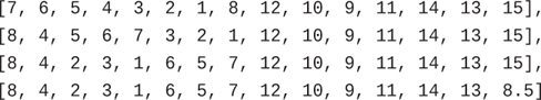
	[7, 6, 5, 4, 3, 2, 1, 8, 12, 10, 9, 11, 14, 13, 15],
	[8, 4, 5, 6, 7, 3, 2, 1, 12, 10, 9, 11, 14, 13, 15],
	[8, 4, 2, 3, 1, 6, 5, 7, 12, 10, 9, 11, 14, 13, 15],
	[8, 4, 2, 3, 1, 6, 5, 7, 12, 10, 9, 11, 14, 13, 8.5]
8.5 Every binary tree can be represented as an array, as described in the section titled “Trees Represented as Arrays.” The reverse of representing an array as a tree, however, works only for some arrays. The missing nodes of the tree are represented in the array cells as some predefined value—such as None—that cannot be a value stored at a tree node. If the root node is missing in the array, then the corresponding tree cannot be built. Write a function that takes an array as input and tries to make a binary tree from its contents. Every cell that is not None is a value to store at a tree node. When you come across a node without a parent node (other than the root node), the function should raise an exception indicating that the tree cannot be built. Note that the result won’t necessarily be a binary search tree, just a binary tree. Hint: It’s easier to work from the leaf nodes to the root, building nodes for each cell that is not None and storing the resulting node back in the same cell of the input array for retrieval when it is used as a subtree of a node on another level. Print the result of running the function on the following arrays where n = None. The values in the array can be stored as either the key or the value of the node because the tree won’t be interpreted as a binary search tree.

[],
[n, n, n],
[55, 12, 71],
[55, 12, n, 4],
[55, 12, n, 4, n, n, n, n, 8, n, n, n, n, n, n, n, n, 6, n],
[55, 12, n, n, n, n, 4, n, 8, n, n, n, n, n, n, n, n, 6, n]