

10
Trees
Objectives
An introduction to rooted and unrooted trees
An introduction to spanning trees
Code and data structures for representing trees
Code and data structures for representing binary trees
The heap structure as a tree structure
Preorder, postorder, and inorder traversal of a tree
Key Terms
ancestor of a node
balanced tree
binary tree
breadth-first search
breadth-first traversal
bush factor
children
complete binary tree
complete ternary tree
decision tree
depth-first search
depth-first traversal
depth of a node
embarrassingly parallel
greatest common divisor
heap
heap property
height-balanced
height of a binary tree
height of a node
inorder traversal
interior node
leaf node
left child
level of a tree
level traversal
load balancing
max-heap
min-heap
objective function
parent
postorder traversal
preorder traversal
right child
root
spanning tree
tree
tree traversal
unrooted tree
221

222 CHAPTER 10 TREES
Introduction
In the previous chapter, we covered the basic notion of a graph and the formal
definitions needed to discuss graphs in a precise way. We will cover general graphs
in a later chapter. This chapter, however, is devoted to a special kind of graph
called a tree because organizing data and information into trees is ubiquitous in
computing. You have already used trees any time you have used a modern computer,
and now we will discuss how to create and use trees in programs.
10.1 Trees
There are many equivalent definitions of a tree. We will define a tree to be a con-
nected graph with n nodes and n −1 edges. We will equivalently use the definition
that a tree is a connected graph with no cycles. We will leave the proof that these
two definitions are equivalent as an exercise.
Perhaps the most obvious tree is a family tree of one’s parents, grandparents,
and so forth (assuming no incest or other unusual circumstances). Each person has
two biological parents, who are distinct nodes in the tree. Each parent has two
parents, who are distinct, and so forth.
As defined here, a tree is not viewed as a “directional” object. However, if we were
to think of an evolutionary tree from a common ancestor, we would probably view
the common ancestor at “the top” and the descendants hanging “down” from the
top. Conversely, if we were thinking of our own descent from parents, grandparents,
etc., we would probably place the root of the tree (ourself) at the bottom and
extend our ancestors upward back in time. Note that there are many examples of
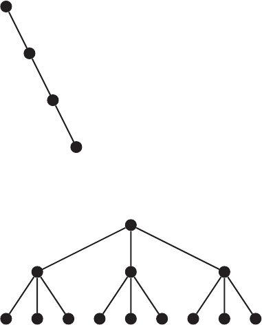
unrooted trees that have no obvious focal point. Figure 10.1 is a general tree with
no identifiable root. Figure 10.2 is a less general tree, with an identifiable root at
the top of the figure and the children of each node hanging down from the parent
node. Continuing the analogy with a family tree, for any node v, we refer to any
parent, grandparent, great-grandparent, etc., node as an ancestor node.
We refer in a tree to the nodes with only one edge incident upon them as leaf
nodes. Whether the tree is displayed in a directional manner, like a family tree, or
without direction or root, the notion of a leaf is obvious. If one is traversing the
tree by using the edges to move from one node to another, then once one comes to
a leaf, there is no place to go except to return along the edge just traversed to the
node from which one just came. A node that is not a leaf node is referred to as an
interior node. In the tree in Figure 10.1, nodes a, c, h,andi are leaf nodes and the
rest are interior nodes.
As you might imagine, dealing computationally with unrooted trees is more com-
plicated than dealing with rooted trees. There is, for example, no obvious starting
10.1 Trees 223
a
c
d
e
f
g
h
i
b
FIGURE 10.1 A general unrooted tree.
FIGURE 10.2 A general rooted tree.
point from which to traverse an unrooted tree, nor is it obvious how we might
use the intuitive two-dimensional layout of the tree to our advantage. In contrast,
most tree algorithms make heavy use of the concept of the root of the tree. In a
game-playing program, for example, the root represents the starting point of the
game, the first level “down” the choices of opening moves, the next level “down”
the choices of responses to the opening moves, and so forth. Further, we can make
heavy use of the two-dimensional layout with the idea of progressing “down” from
the root and of working “left” to “right.”
Given a rooted tree such as in Figure 10.2 (which we have already seen in
Figure 9.1), the height and depth of a particular node in the tree are defined as
follows. The depth of a node v is the number of edges between v and the root of the
tree, that is, the number of ancestors of v, not including the node v itself. Given
that a tree is a graph with no cycles, there is only one path from any given node
to the root, and the depth of a node is the length of that path. We can also define
224 CHAPTER 10 TREES
this recursively: the depth of the root is 0, and the depth of a nonroot node is 1
plus the depth of the node’s parent.
The depth of a node is the measurement of its distance from the root. The
height of a node is the distance in the opposite direction, that is, the distance
to the farthest leaf node. We must be a little more careful, however, in defining
the height than in defining the depth because not all trees are balanced. A tree is
balanced if no leaf node is “much farther” away from the root than any other leaf
node. As should be obvious, this isn’t a precise definition due to the vague nature
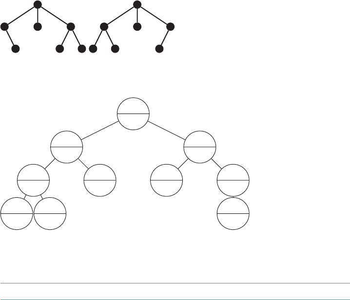
of the “much farther” part. Clearly, the tree in Figure 10.3 should be viewed as not
being balanced, and the tree in Figure 10.4 should be viewed as being balanced. In
most contexts, however, we would also consider the trees in Figure 10.5 both to be
balanced and for many (but not all) purposes equivalent.
In general, as we shall see later in this chapter and in Chapter 12, we want our
trees to be balanced because processing on balanced trees is more efficient.
FIGURE 10.3 An unbalanced tree.
FIGURE 10.4 A balanced tree.
Thus: The height of a leaf node is 0, and the height of a nonleaf node v is 1 plus
the maximum of the heights of all the children of v. This is illustrated in Figure 10.6.
Finally, we will refer to all the nodes of depth n as level n of that tree.

10.2 Spanning Trees 225
FIGURE 10.5 Equally balanced trees?
d = 0
h = 3
d = 1
h = 2
d = 2
h = 1
d = 3
h = 0
d = 3
h = 0
d = 2
h = 0
d = 1
h = 2
d = 2
h = 0
d = 2
h = 1
d = 3
h = 0
FIGURE 10.6 Depths and heights.
10.2 Spanning Trees
A common problem in computing is to compute a spanning tree for a more general
graph. Given a general graph, a spanning tree would be a tree that includes all the
nodes in the graph and a subset of the edges that connect the nodes into a tree. Just
as a phone tree allows an organization like a political action committee to reach all
its members by having members call members who then in turn call more members,
a spanning tree is often constructed when it is necessary to create a communica-
tions backbone that would reach all the nodes in a graph. This is an increasingly
important computation in setting up networks of wireless devices. Such devices
change position relative to each other and relative to the fixed communications
towers through which they communicate, so efficiently establishing networks for
what amounts to a conference call among mobile devices has become an important
problem to solve.
Figure 10.7 shows a spanning tree with dashed edges indicating the spanning tree
and colored edges indicating other edges in the graph. We will discuss algorithms
for spanning trees in Chapter 13.

226 CHAPTER 10 TREES
FIGURE 10.7 Two spanning trees (dashed) for the same graph.
10.3 Data Structures for Trees
One can easily implement a tree using almost the same code as one uses for a
linked list. Indeed, most of the structures in this text follow the hierarchy of a data
structure class, which contains instances of a node class in the structure with each
node class containing a data payload. The primary changes, from one structure to
the next, in the node class are in the connections from one node to the next that
implement the data structure one level higher up.
In the case of linked lists to implement linked lists, stacks, and queues, the
nodes have a next and a previous pointer. With a node in a tree, there will be a
parent pointer that points “up” and some number of children pointers that will
point “down.” The complication that arises in dealing with trees is that a tree is a

10.3 Data Structures for Trees 227
public class TreeNode
{
private TreeNode parent;
private ArrayList<TreeNode> children;
private DataPayload data;
// constructors
// accessors
// mutators
// other methods
} // public class TreeNode
FIGURE 10.8
A code stub for a tree node.
TreeNode
-parent:TreeNode
-children:ArrayList<TreeNode>
-dataPayload:Record
+ accessors
FIGURE 10.9 UML diagram for a tree node.
two-dimensional object, not a one-dimensional object like an array or ArrayList.
Also, since the number of children of any given node is variable, we need a variable-
length structure like an ArrayList or a linked list in which to store the pointers
to the children. A TreeNode in Java might therefore have a stub that looks like
Figure 10.8 and a UML diagram that looks like Figure 10.9. This is really only
a very slightly different structure from the node for a linked list, stack, or queue.
Instead of a previous node, we have a parent node. Instead of a single next node
for a given node, we have zero or more children nodes that hang down from a given
node and can be stored in an ArrayList. Since an ArrayList imposes a natural
order (the subscripting) on its entries, we would naturally think of the sequential
ordering of child nodes in the ArrayList as being the same as our graphical layout
of the tree on paper, as indicated in Figure 10.10. In traversing a linked list, we
used next and previous to make a linear traversal. If we want to make a similar
traversal of all the nodes in a tree, we will now have to run a loop over the list of
children entries in the ArrayList.
Clearly, if we wanted to, we could use the Iterator concept to implement a
structure that hides the TreeNode from the programmer. This will, of course, be
harder to do with a tree than with a stack or queue because the notion of the “next”
item is no longer unique.

228 CHAPTER 10 TREES
A
B, C
B
D, E
D
J, K
J K
E
ø
øø
øøøø
C
F, G ,H
F
L
L
G
M
M
H
N, O
N O
FIGURE 10.10 Node labels (top) and ArrayList children (bottom).
10.4 Binary Trees
In many situations a general tree is needed because one cannot control or specify
in advance the number of children for any given node.
1
However, there are many
situations in which the program design or the algorithm can be imposed upon the
data, and in many of these situations what is needed is a binary tree,atreein
which each node has at most two children.
We have already seen binary trees appear in (at least) two different contexts—
the heap structure for a priority queue and the binary decision structure of binary
search.
A particular use of binary trees comes in these two situations—when the tree
structure is used for adding the ability to search or sort some data or the binary
tree is either explicit or implicit as part of a divide-and-conquer algorithm. Since
we have at most two children, we can refer explicitly to the left child and the right
child of a given node, with left and right determined by the visual placement of the
nodes when the tree is displayed in standard position as in Figure 10.11.
Almost invariably, if we are referring to a tree as a binary tree, we will retain the
right-child or left-child layout even if one of the two nodes is missing. That is, even
if we have missing nodes, we will display the tree as in Figure 10.12 rather than as
in Figure 10.10 with the single nodes dropping straight down from the parent. For
some binary trees, such as the binary search trees we will discuss in Chapter 12, the
left-ness or right-ness has meaning, so maintaining the missing node as a missing
right node or a missing left node is required.
1
For example, if this is a family tree and the children really are children.

10.4 Binary Trees 229
1
2
4
8 9
5
10 11
3
6
12 13
7
14 15
FIGURE 10.11 A binary tree.
1
2
5
10 11
3
6
13
FIGURE 10.12 A binary tree with missing nodes.
Wecallabinarytreecomplete if every interior node has exactly two children.
As one can easily see, a complete binary tree with n levels will have exactly 2
n
− 1
nodes and 2
n−1
leaf nodes. We define the height of a binary tree to be the maximum
distance from the root of the tree to any leaf. In some instances we will relax slightly
the definition of complete binary tree to allow for a partial row of leaf nodes,
provided that the partial row of leaves is the “bottom” row and that the “missing”
nodes are all at the right-hand edge of this bottom row, just as we specified earlier
in the case of a heap for a priority queue. If the purpose of calling a tree “complete”
is to refer to the fact that there are no holes in the display, then clearly there is
more justification for calling the tree in Figure 10.16 complete than there is for the
tree in Figure 10.12, which clearly has holes in the middle.
10.4.1 Implementing Binary Trees with Nodes
To implement a binary tree we can use a program stub like the code in Figure 10.13
for the nodes in the tree; the fixed nature of one parent and two children (one or

230 CHAPTER 10 TREES
public class BinaryTreeNode
{
private BinaryTreeNode parent, leftChild, rightChild;
private DataPayload data;
// constructors
// accessors
// mutators
// other methods
} // public class BinaryTreeNode
FIGURE 10.13
A code stub for a binary tree node.
both of which may be NULL) make this look very much like the node for a linked
list. All the complications that arise from the possibility of a variable number of
children disappear, and we do not need the variable-length ArrayList of a general
tree. One might also wish to include an instance variable sibling that points to
the rightChild of the parent if one is a leftChild and to the leftChild of the
parent if one is a rightChild. Knowing who the sibling is can be useful (as in the
heap discussed later), but in a minimalist implementation of a binary tree a node
might not know whether it is the right or the left child of its parent.
A word about programming style is relevant here. In developing code for a general
tree, we have almost no choice but to use an ArrayList to store the children of
a node because we don’t know how many children, if any, will exist. Processing
of children nodes will probably take place in subscript order in the ArrayList
because the natural way to deal with an ArrayList is with a simple loop. With
a binary tree, we have the option of explicitly labeling child nodes as either left
or right. Although this can make the code easier to read (because the text of the
code will specifically say “left” or “right”), it can also lead to duplication of code
segments, which could lead to errors. It also means that general-purpose tree code
will be much different from binary tree code. A middle ground might be to use
the general-purpose tree code with an ArrayList for storing children but to build
into that code additional safeguards to ensure that no node mistakenly is assigned
more than two children. Since the ArrayList would likely be processed in subscript
order, the code documentation should point out that the abstract subscript order
(0, 1) should match up as (left
child, right child), and this can be facilitated
by defining final constants LEFT
CHILD = 0 and RIGHT CHILD = 1 to ensure that
the code has no magic numbers. To Einstein is attributed the statement, “Make
everything as simple as possible, but not simpler.” In writing code, there is always
the need to find a middle ground between explicit code that is very readable but can

10.4 Binary Trees 231
be buggy because it is overly verbose and general-purpose code that is smaller but
less readable because it is less explicit, and thus can be buggy because it requires
more concentration to ensure correctness. Your mileage may vary. If circumstances
permit, it is often better to write the explicit version first to get the output correct
and then to write the general-purpose version. In that way, when you write the
general-purpose version with more abstraction and chance for error, you will have
correct results to use for diagnosing the errors.
10.4.2 Implementing Binary Trees with Arrays
In implementing a general tree, we have no way apriorito determine a sequence
number for a given node because the number of child nodes is variable. This is
an example of the local–global information issue we commented on in the previous
chapter; we cannot look locally at a given node in a tree and determine a proper
sequence number for that node without looking globally at the rest of the tree. For
example, viewing the tree in Figure 10.14 as a general tree, we can look globally
to determine that the three nodes on the bottom level should be numbered 4, 5,
and 6, but it requires global information and some sort of indexing scheme to be
able to point definitively to a specific node as the child of some other specific node.
Consider the tree in Figure 10.14 with nodes labeled as array subscripts working top
to bottom and left to right. If we were to store the nodes in an array or ArrayList
of nodes, we would need an auxiliary index array such as
index =[1, 4, NULL, 5, NULL, NULL, NULL]
to indicate that the children of the root node (which is subscript 0) begin at sub-
script 1, the children of the node at subscript 1 begin at subscript 4, and so forth. If
our only means for chasing down the paths of a tree were to run through the array
of nodes, we would also need to determine the number of children for any node. For
example, we would be able to determine that the child nodes of the root begin at
index[0] = 1 and end at index[1] − 1 =3.
0
1
4
2 3
5 6
FIGURE 10.14 A hard-to-subscript tree?

232 CHAPTER 10 TREES
In contrast to this situation with general trees, we can with binary trees establish
a fixed subscripting mechanism using an array (or an ArrayList). This is exactly
what we did for the heap in Chapter 7.
The complete binary tree in Figure 10.11 has been deliberately subscripted
1-up instead of 0-up so as to map the nodes into a linear array with the sub-
scripts matching up cleanly. In Java, which subscripts 0-up, an implementor would
have to adjust subscripts accordingly or else just decide to waste the zeroth storage
location but gain the advantage of code that was easier to read.
With this choice of subscripting, the left child of the node at subscript i will be
the node that has subscript 2i,andtheright child of the node at subscript i will
be the node that has subscript 2i + 1, as can be seen by comparing the table in
Figure 10.15 against the tree in Figure 10.11. Level k in such a tree will have nodes
subscripted 2
k
through 2
k
− 1, which is clearly easier to work with than it would be
with 0-up subscripting and nodes at level k having subscripts 2
k
− 1 through 2
k
− 2.
Subscript Tree Level Node
1 0 v
1
2 1 v
2
3 1 v
3
4 2 v
4
5 2 v
5
6 2 v
6
7 2 v
7
8 3 v
8
9 3 v
9
10 3 v
10
11 3 v
11
12 3 v
12
13 3 v
13
14 3 v
14
15 3 v
15
FIGURE 10.15 Mapping a binary tree into an array.
Of course, we can implement any tree with a fixed maximum on the number of
child nodes using exactly this subscripting algorithm for array subscripts. However,
the potential benefit from using an array diminishes if a large number of the array
locations wind up not being filled. Only if a tree is reasonably complete will the
advantage of the array with simple subscripting and access to nodes overcome the
added cost of memory space that is allocated but not used.
10.5 The Heap 233
10.5 The Heap
Most of the time, the algorithmic and implementation issues involved in turning
an idea into program code are relatively straightforward, often being simply the
commonsense conclusion from looking at the problem in the right way. As we saw
in Chapter 7, though, one structure that appears to add some almost-magical extra
value is the heap. We have already seen a heap used for a priority queue in Chapter 7,
and we will use the heap in Chapter 11 to implement the heapsort.Someofwhat
is presented here has already been presented in Chapter 7. That’s OK—this is a
concept so important that it is worth explaining it in two different ways.
Let’s repeat the definition but this time in the terminology of trees. A binary
tree whose nodes carry data payloads that have comparable numerical values is said
to satisfy the heap property if for all nodes other than the root we have
thisNode.getValue() <= thisNode.getParent().getValue()
that is, if the data payload value stored at any given node is less than or equal
to the payload value stored at the parent node. A binary tree that is complete
except possibly for missing nodes on the right-hand edge of the lowest level, and
all of whose nodes satisfy the heap property, is called a heap. Figure 10.16 shows a
complete binary tree that is a heap.
(1)104
(2)93
(4)17
(8)13 (9)2
(5)82
(10)71 (11)69
(3)76
(6)65
(12)63 (13)61
(7)71
(14)70
FIGURE 10.16 A heap.

234 CHAPTER 10 TREES
We note that in a heap,
2
whose data payload values are nonincreasing from the
root “down” to any leaf node, the maximum value (which need not be unique)
would be stored as the payload in the root.
The power of the heap as a data structure comes in large part from Theorems 7.1
and 7.2. The first asserts that we can create a heap in O(N lg N) time, and the second
asserts that we can add or delete an item and then rebuild the heap in O(lg N) time.
10.6 Traversing a Tree
The basic notion of a tree is ubiquitous in computer science because it is such a use-
ful concept. In many instances, such as with a priority queue, the two-dimensional
structure of a tree can be used as added information to a one-dimensional array
and thus be used to maintain at low cost a structure from which the minimum (or
maximum) entry needs to be extracted and then replaced.
Equally important is the concept of traversing a tree. One canonical example
of tree traversal comes in thinking of a game-solving program for a puzzle such as
Sudoku. We start with a set of open squares and some rules about whether or not
a given number can be placed in one of those open squares. Starting at a dummy
root node (the starting position), we can choose a large number of possible first
moves. For each of those, there is another large set of possible moves, each of which
must take into account the fact that our first move also limited the ability to make
certain second moves by taking out of consideration moves that would reuse the
number of our first choice in that row, column, or subsquare.
Looked at in this way, what we have for a given Sudoku puzzle is a decision
tree of the possible moves: “If X is our first move, then we have a different set of
possible second moves, and we choose move Y from among the possible choices.
This provides us with a set of possible third moves, from which we choose Z....”
If we have a properly formulated puzzle, there will be some decision tree that leads
to a unique solution. That is, if we were to lay out the entire tree graphically, then
a particular choice that was legal at level n but that could not be completed to a
legal solution would have no children at level n +1.
Such decision trees are commonplace both in life and in computer science. Given
the decisions we make, the options open after a given decision are changed, leading
to a set of options for the second decision. If we are to analyze properly what the
tree looks like, then we need to know how to traverse the tree, that is, to visit all the
nodes of the tree in some predefined order. In what follows, all traversal methods
except for inorder traversal make sense for any tree. Inorder traversal makes sense
only for binary trees. And although any tree can be traversed, a complete binary
2
Actually, this is a max-heap because we insist that the data value for the parent is greater
than that of the child. This property forces the overall maximum value to be in the root node of
the tree. If we reversed the inequality, we would have a min-heap.

10.6 Traversing a Tree 235
tree is used as our canonical example. For preorder and postorder traversal of
general trees, one should do the obvious generalization in the algorithms that follow:
replace the “recursively visit the left subtree ...recursively visit the right subtree”
instruction with “recursively visit subtrees from left to right.”
We will use the complete binary tree with labels that was presented in
Figure 10.11.
Algorithmically, the preorder traversal, postorder traversal,andinorder traversal
are done as follows:
Preorder traversal:
visit the root
recursively visit the left subtree
recursively visit the right subtree
Postorder traversal:
recursively visit the left subtree
recursively visit the right subtree
visit the root
Inorder traversal:
recursively visit the left subtree
visit the root
recursively visit the right subtree
If we execute a preorder traversal of the tree in Figure 10.11, we will visit the
nodes in the sequence shown in Figure 10.17.
1, 2, 4, 8, 9, 5, 10, 11, 3, 6, 12, 13, 7, 14, 15
2(2)
3(9)
6(10)5(6)
11(8)10(7)9(5)8(4)
4(3) 7(13)
12(11) 13(12) 14(14) 15(15)
1(1)
FIGURE 10.17 Preorder traversal of a binary tree.

236 CHAPTER 10 TREES
If we execute a postorder traversal of the tree in Figure 10.11, we will visit the
nodes in the sequence shown in Figure 10.18.
8, 9, 4, 10, 11, 5, 2, 12, 13, 6, 14, 15, 7, 3, 1
1(15)
2(7)
5(6) 6(10)
3(14)
7(13)
15(12)12(8) 13(9) 14(11)
4(3)
8(1) 9(2) 10(4) 11(5)
FIGURE 10.18 Postorder traversal of a binary tree.
If we execute an inorder traversal of the tree in Figure 10.11, we will visit the
nodes in the sequence shown in Figure 10.19.
8, 4, 9, 2, 10, 5, 11, 1, 12, 6, 13, 3, 14, 7, 15
You have in fact seen these traversals before but perhaps not with the formality
of these names. Consider an arithmetic expression, such as
5+(3+2+1)∗ (6 + 7) + 26/2.
Although the usual MDAS (My Dear Aunt Sally) rules for performing Multipli-
cation and Division before Addition and Subtraction would apply here, the rules
usually applied in algebra are not the left-to-right rules used by most compilers, so
we will insert extra parentheses to be completely unambiguous:
{5+[(3+2+1)∗ (6 + 7)] + (26/2)}.
This expression can now be written as a tree as shown in Figure 10.20 and the
evaluation of the expression, inside out and left to right, is exactly the postorder

10.6 Traversing a Tree 237
1(8)
6(10)
3(12)
12(9) 13(11) 14(13) 15(15)
7(14)
2(4)
4(2)
8(1) 9(3) 10(5)
5(6)
11(7)
FIGURE 10.19 Inorder traversal of a binary tree.
+
+
+
+
5
3 2
1
+
6 7
/
26 2
∗
FIGURE 10.20 An arithmetic expression tree.
traversal of the tree, especially if we view the evaluation of the expression in the
same way we looked at stack processing in Chapter 7. Processing is essentially
inside out: we visit the 5 node first and then must progress down the right child
path to the leaves containing 3 and 2. Having visited both children and collected
the arithmetic arguments in doing the visit, we can visit their parent, the +, and
add 3 + 2 to get 5. We then visit the right child to pick up the 1, and then the root
(again a +) to add 5 + 1 to get 6. And so forth. Some of the successive stages of the

238 CHAPTER 10 TREES
+
5
3 2
1 6 7
/
26 2
5
5 1 6 7
/
26 2
+
+
+
+
+
+
+
+
∗
∗
FIGURE 10.21 Postorder processing of an arithmetic expression tree, part 1.
postorder processing are shown in Figures 10.21–10.23. (Not all the individual visits
are shown in order to save some space, and we don’t run the processing through to
the final result.)
In covering the use of a stack in Chapter 7, we discussed XML or HTML tree
structures, which very closely resemble arithmetic expressions. In fact, there are
extensive standards for laying out web pages and XML documents as trees so
that standard software packages can process the trees. One of these standards is
the DOM, or Document Object Model, and there are standard packages in many
programming languages (including Java) that will read web pages and XML doc-
uments, create a tree much as we have created trees for arithmetic expressions or
XML, and provide methods for navigating the tree and processing the document. It
should be clear that if the XML tree structure were analogous to Figure 10.20, then
the processing of the XML would be analogous to evaluating an algebraic expression.
We will see in Chapter 12 a use for inorder traversal of a tree.
We presented postorder processing as one version of the use of a stack for pro-
cessing algebraic expressions or nested markups in a markup language like HTML
or XML. Somewhat similar examples of preorder processing can be found. We
10.6 Traversing a Tree 239
5
5 1 6 7
/
26 2
+
+
+
5
∗
6
6 7
/
26 2
+
+
+
+
∗
FIGURE 10.22 Postorder processing of an arithmetic expression tree, part 2.
described the greatest common divisor function back in Chapter 8. We can also
define a recursive gcd function as follows.
int gcd(int a, int b)
{
if(a == b)
return a;
else if(a < b)
return gcd(a, b-a);
else if(a > b)
return gcd(a-b, b);
}
This definition and method rely on the (easy to prove) fact that
gcd(a, b)=gcd(a, b − a)=gcd(a − b, b),
with suitable special cases for negative integers, zero, and such. In Scheme, which
is a variant of LISP,
3
both of which are languages used for many years now in
3
Both “Lisp” and “LISP” seem to be in common usage. What is true for both is that the
acronym could possibly stand for “Lots of Irritating Single Parentheses”; counting up the right
number of nested parentheses has always been difficult.

240 CHAPTER 10 TREES
5
6
6 7
/
26 2
+
+
+
∗
5
6 13
/
26 2
+
+
∗
FIGURE 10.23 Postorder processing of an arithmetic expression tree, part 3.
artificial intelligence and compiler writing, the greatest common divisor function
canbewrittenasfollows.
(define gcd
(lambda (a b)
(cond ((= a b) a)
((> a b) (gcd (- a b) b))
(else (gcd (- b a) a)))))
The Scheme language is intended to be parsed in a preorder fashion. The define
keyword becomes the root of the tree, the gcd name of the function is the left
child of the root, and the function itself is the subtree whose root is the right child,
beginning with the keyword lambda. Then lambda istherootofasubtreewith
the parameters abas the left child and the rest of the expression as the right
child. Even if you don’t know Scheme (and you probably don’t, which is perfectly
OK until you take the programming languages course later in the curriculum),
it’s possible to see that keywords (or function names or operators) like gcd are
followed by two arguments, both of which could be entire subtrees. All this is entirely
analogous to the postorder processing of algebraic expressions; the real difference is
that with algebraic expressions and a stack one waits for an operator to appear and

10.6 Traversing a Tree 241
then applies that operator to the top two arguments on the stack. With algebraic
expressions, it is easy to think inside out, in a postorder fashion. With LISP or
Scheme, the intent is that one thinks top-down, with a preorder mindset.
10.6.1 Breadth-First and Depth-First Traversal
There are two other traversal methods for trees (or more generally for graphs). A
depth-first traversal is essentially the same as an inorder traversal. The order in
which nodes are visited is the same (left subtree, root, right subtree), but a depth-
first traversal is used in many instances as part of a depth-first search, which will
be discussed in the next chapter. There are two variations of depth-first search that
come immediately to mind if the tree represents, for example, a game strategy.
First, we might probe paths of game moves, starting with the leftmost unexplored
path, all the way to the end of the game to determine whether or not that path
was a winning strategy. In the case of a naive Sudoku solver, with each level being
a specific square to fill in and each node branching out to nine possible choices for
that square, we would encounter a very large number of search “crash” conditions
for illegal choices, and the entire tree below the node giving the crash would be
pruned away; we wouldn’t actually have to probe all the way to the end of the
game. One can imagine that this would be a simple program to write because it
would be a recursive call to a method that ran a couple of loops, and also that
it would be very inefficient because a large number of the paths would be illegal.
The program would spend most of its time in worthless looping and testing of
possibilities already shown to be illegal. We note that in this kind of search the
interior nodes don’t really have a part to play. Unlike the tree in Figure 10.20, in
which the interior nodes were the operations to be performed on the data in the
child nodes, in this kind of search the interior nodes contain no information other
than “more work to do” or “all subpaths already examined.”
The other kind of depth-first search tree is exemplified by a game such as chess. In
chess, there are too many possible moves to be able to explore any path all the way
to the end, but we also have, based on the knowledge of experts, a way to quantify
the “goodness” of any given board position. If we were to consider one move on
our part and then one response by the opponent, we could calculate the board’s
“goodness” for each move and response, and the purpose of our tree search would
be to choose our move so as to maximize the goodness. The goodness (or badness,
depending on one’s point of view) function is referred to in this kind of search as
an objective function to be minimized or maximized depending on the details.
The naive depth-first search, then, would probe down as many levels as was fea-
sible (competition chess games are timed, after all), compute the objective function
for the leaves at that level, and then minimize or maximize the objective function
as needed by applying a min or max function in the interior nodes of the tree.

242 CHAPTER 10 TREES
In a breadth-first traversal, also called a level traversal, the nodes of the tree in
Figure 10.11 are visited in order
1, 2, 3, 4, 5, 6, 7, 8, 9, 10, 11, 12, 13, 14, 15
that is to say, all the nodes of level 0, followed by all the nodes of level 1, all the
nodes of level 2, and so forth. In a complete binary tree, especially one that is stored
in an array or ArrayList with subscripts, breadth-first traversal is relatively sim-
ple because there is a static assignment of nodes to subscripts as in Figure 10.15.
For a general tree, however, or one that is maintained simply as nodes with links
to parents and children, there isn’t enough information to allow one to conve-
niently perform breadth-first search. For example, we have no way to determine
the breadth-first successor to node 9 in Figure 10.11 without knowing more about
the position of node 9 in the overall tree. The same is true of nodes 5 and 11. Think
back to our comments about local information and global information: in order
to process breadth first, we need more information about depth and position. A
further complication arises if we have a dynamic tree with additions and deletions
occurring. Let’s assume that we include in a tree node the links going right and
left that would make the nodes at a given level into a doubly-linked list. If we now
allow a node (say node 5) to be deleted, we must now adjust the doubly-linked lists
at the level of node 5 and at the levels of all its children. Although this may be
entirely appropriate in some situations, it also starts looking like a complication for
which some other data structure might be more appropriate.
10.6.2 Traversal on Parallel Computers
It frequently happens that tree traversal is a computationally expensive proposition
because game trees can be very large. In any serious game, such as chess or go, the
total number of possible move-and-response paths is huge, making an exhaustive
search impossible. Even for something as simple as Sudoku, it can be prohibitively
expensive in CPU time to pursue a naive search through trial and error. Because
searching in decision trees is an important application but is computationally expen-
sive, it is often done on parallel computers, in part because searching on a decision
tree is an embarrassingly parallel process. A problem is referred to as embarrassingly
parallel if it is absolutely trivial to sketch out an approach for doing independent
parts of the computation in parallel with each other.
4
Consider a totally naive program for Sudoku. There are 81 total squares, and in a
medium-difficult puzzle there might be about 31 of these filled in. Since each square
4
It is commonplace at this point for those in parallel computing to point out that they are not
at all embarrassed to work on problems that are embarrassingly parallel.

10.6 Traversing a Tree 243
could be filled in with one of the digits 1 through 9, there are 9
50
≈ 5.15 · 10
47
possible solutions that could each be checked in parallel, since each of these is
completely independent of one another. We have naively a 9-ary tree of 50 levels
representing the possible decision trees toward a solution to the puzzle. We start at
the root of the decision tree, choose an empty square S
ij
, and farm out the work
to nine different processors P
1
through P
9
. Each processor P
k
will check whether
k is a legal value in square S
ij
; if so, it will assign k to the square and recursively
farm out the test for the next square to nine more processors.
We obviously aren’t going to solve the Sudoku puzzle this way. First, in even the
largest supercomputers we have perhaps 10
5
processors, not 10
47
, so we are clearly
not going to be able to use a different processor to test each possible solution.
Second, spawning a parallel process to test a solution almost certainly takes a lot
more work than does the simple test of whether the possible solution actually works,
so using one processor for one test incurs an enormous waste in overhead. Finally,
it is obvious that huge parts of the game tree don’t have to be explored—for every
value that fails to be possibly valid in the choice at the first level, 1/9 of the entire
tree can be pruned away. If we don’t take this into account in assigning processors
to tests, we will waste processors by having them sit idle.
What invariably happens in doing a search through a tree on parallel processors
is as much art as it is science, and it is to perform a hybrid of breadth-first and
depth-first search, with the parallel processors self-scheduling their work off a task
queue. The task queue in steady state will be a partial puzzle board and a list
of “some number” of “the next” squares to be tested. If a single processor can
reasonably handle exhausting the 9
6
possibilities of a complete search through six
levels, then the value of “some number” will be set to 6. In steady state, then, each
processor will pull a task off the task queue and will conduct a six-level depth-first
exhaustive search. Every partial board for which six new squares can be assigned
values will become a new task appended to the task queue. The processor will
then take another task off the top of the task queue and continue. Locally, on
each processor, a depth-first exhaustion of the tree is performed. Globally, if all the
tasks were to take exactly the same amount of time, then the parallel assignment
of tasks to a block of processors would resemble a breadth-first search. We would
be assigning a block of processors to a horizontal set of nodes or tasks at a given
level every time, thus progressing across the level in blocks.
The “art” in this kind of computation involves ensuring load balancing so that an
individual task is an efficient computation and the cost of spawning processes and
managing tasks is small compared to the cost of computing depth-first chunks of the
tree. If the “some number” of levels is too small, we waste processor time in startup
and shutdown activities. If the number of levels is too large, we run the risk of having
an inefficient local computation (more tests often means more memory used) and

244 CHAPTER 10 TREES
insufficient parallelism. The “science” is generally just the general principles; the
art comes from knowing detailed costs for the machine on which the computation
will be performed.
10.7 Summary
We have introduced rooted and unrooted trees and the notion of a spanning tree.
Trees are important computational structures, and they can be implemented in
any of several ways, although most general tree structures would be implemented
in Java using an ArrayList to store pointers to the child nodes for any given node.
Binary trees are trees that have at most two children for any given node. Since
binary trees often correspond to binary divide-and-conquer algorithms, binary trees
are often implemented explicitly instead of with the more general code and data
structures.
Another use of a binary tree is to implement a heap.
Finally, we have presented preorder, postorder, and inorder traversals of a tree.
These are the common traversal methods, and each of these is used for specific
important purposes.
10.8 Exercises
1. Show that the two definitions of a tree are equivalent. That is, show that
(a) If a graph on n nodes is connected and has n −1 edges, then it has no
cycles.
(b) If a graph on n nodes is connected and has no cycles, then it has n −1
edges.
2. Identify the leaf nodes and the interior nodes on the graphs in Figures 10.1,
10.2, 10.3, 10.4, and 10.5.
3. (a) Show that a complete binary tree with levels 0 through m has exactly 2
i
nodes at each level i,0≤ i<m,exactly2
m+1
− 1 total nodes, exactly 2
m
leaf nodes, and exactly 2
m
− 1 interior nodes.
(b) A complete ternary tree is a tree in which every interior node has exactly
three children. Show that a complete ternary tree with levels 0 through
m has exactly 3
m
nodes at each level i,0≤ i<m,exactly
3
m+1
−1
2
total
nodes, exactly 3
m
leaf nodes, and exactly
3
m
−1
2
interior nodes.
(c) Develop the general formulas for a complete n-ary tree for any n.
4. Give the preorder, postorder, and inorder traversals of the tree in Figure 10.20.

10.8 Exercises 245
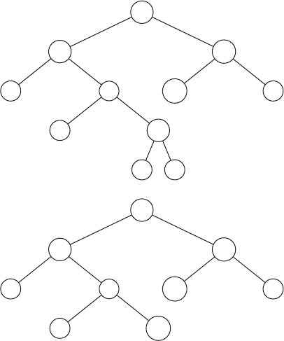
5. Give the preorder, postorder, and inorder traversals of the following tree.
A
B
C
D
E
F
G
H
I
6. Implement a tree in code and use it to process the XML in Figure 7.5.
7. Implement a binary tree in code using an ArrayList and the standard sub-
scripting for a binary tree done as a list. Use it to process the arithmetic
expression in Figure 10.20. If you convert the expression into the explicit list
of nodes and subscripts, you can concentrate on the tree traversal and evalu-
ation of the expression rather than on parsing the expression. The input file
can be found on the website at go.jblearning.com/Buell.
8. Implement a binary tree in code with explicit left and right child nodes. Use
it to process the arithmetic expression of Figure 10.20 just as in Exercise 7.
9. Add a method to any of your tree codes to compute the minimum, maximum,
and average depth of the leaf nodes in the tree.
10. Add a method to any of your tree codes to determine if the tree is height-
balanced. A tree is said to be height-balanced if the maximum and minimum
distance from any node v to any leaf node below v differbyatmost1.Your
method should be recursive because this definition is inherently recursive.
11. Add a method to any of your general tree codes to compute the minimum,
maximum, and average bush factor of a node. The bush factor is the number
of children emanating from a given node in the tree.
12. Given a general tree without a root, such as the following, show all possi-
ble trees that can be constructed from the original tree by adding one more
leaf node. Write a method that will generate from an arbitrary tree all the
augmentations obtained by adding one leaf node.
A
B
C
D
E

..................Content has been hidden....................
You can't read the all page of ebook, please click here login for view all page.