

11
Sorting
Objectives
The concept and implementation of standard sorting algorithms—
bubblesort, heapsort, insertionsort, mergesort, and quicksort
Analysis of the worst-case running times of the standard sorting algorithms
Analysis of the average-case running times of the standard sorting algo-
rithms
The difference between worst-case and average-case running times of algo-
rithms and how to perform an average-case analysis
Practical considerations of sorting: auxiliary space, disk, the extent to which
the input data is already sorted, multilevel sorting, and stability
The lower bound on sorting by comparisons
* Sorting on a distributed memory parallel computer
Key Terms
average-case running
time
best-case running time
bubblesort
bucketsort
distributed memory
parallel computer
in-place algorithm
insertionsort
key
mergesort
out-of-place algorithm
pivot element
quicksort
shared memory parallel
computer
stable sort
worst-case running time
Introduction
It has been asserted by Knuth that perhaps a third of all CPU cycles are spent in
sorting data. This is a huge fraction, but the problem of sorting data comes up in
247

248 CHAPTER 11 SORTING
many circumstances when it might not be so obvious that sorting was important.
Sorting and searching go hand in hand (indeed, Volume 3 of The Art of Computer
Programming by Knuth bears Sorting and Searching as the title), and creating and
maintaining sorted lists, or searchable trees like a priority queue with a heap or a
binary search tree, is enormously important. For example, when a Java program
is compiled, the compiler must do a lookup every time a symbol or variable name
appears. Every time Google does a search, it must process index files. We have
already seen that in the absence of some means for creating a sorted or search-
able list, the time needed to find a single record among N records is, on average,
O(N/2), which is expensive. With binary search on a sorted or indexed file, as in
our FlatFile example, or with a binary search tree, that cost can be reduced to
O(lg N). With a heap used as a priority queue, we can extract the most important
entry and then rebuild the heap structure in O(lg N) time.
As is customary, we will refer to sorting keys under the assumption that our data
record, which might be an entire student transcript, is to be sorted based on the
value of some key, like the student’s ID number. Although it sometimes happens
that there is an assigned key for a record, like an ID number or a Social Security
number, it is often the case that the key is constructed from data in the record.
For example, one might try to construct as unambiguous a key as possible from
last name, first name, and middle name (probably in that order) when sorting an
address book. This involves some art rather than science, and perhaps also some
rules for deciding how to alphabetize. We will gloss over somewhat the process of
creating the key and simply assume that keys can be created based on a set of rules.
Our interest is in how to use the keys in sorting algorithms.
11.1 Worst-Case, Best-Case, and Average-Case
In this chapter we will, for the first time, explore more deeply the issue of worst-
case running time versus average-case running time and best-case running time.For
the purpose of doing asymptotic analysis, we always concentrate on the worst-case
running time, and we would like to discover algorithms that are fast even in the
worst case. However, as we shall see with quicksort, an algorithm that has a good
average-case behavior might be preferable if its implementation takes advantage of
other factors beyond simple asymptotics. The usual goal, after all, is to sort, not
to prove theorems about how one might sort.
Under some circumstances we might also look at the best-case behavior of an
algorithm. We can’t write code as if we are going to encounter the best case in
practice, but we can learn sometimes from best-case behavior. For example, there
are some sorting algorithms that are fixed-cost algorithms, taking always the same
11.2 Bubblesort 249
length of time regardless of the nature of the input data. Some algorithms, though,
are much more effective on almost-sorted data than they are on random data. The
algorithm chosen to sort a large file that is known to be nearly sorted to begin with
will probably be different from the algorithm chosen to sort a file of data about
which we know nothing.
11.2 Bubblesort
The simple version of code for a bubblesort,asusedintheIndexedFlatFile
example, is given in Figure 11.1.
public void bubblesort()
{
for(int length = this.getSize(); length > 1; --length)
{
for(inti=0;i<length-1; ++i)
{
if(record[i] > record[i+1])
{
CODE TO SWAP record[i] WITH record[i+1]
}
}
}
}
FIGURE 11.1
Code fragment for a bubblesort.
As should be clear by now, this is an O(N
2
) computation. The outer loop iterates
N −1 times. In the first iteration of the outer loop, the inner loop iterates N − 2
times. In the next outer iteration, the inner loop iterates N − 3times,andsoforth.
This is a total of
(N −1) + (N − 2) + ···+1=
(N −1)N
2
= O(N
2
)
iterations of the inner loop code to compare and perhaps swap two records based
on comparing the values of their keys.
This algorithm works because in each iteration of the outer loop we exchange
pairs, bubbling the largest element down the list into the current “last” position,
and by the time we have finished the ith iteration, the element in the ith location
from the end is the ith largest of all elements. With each outer loop iteration, then,
we fix only one more element into its proper place.

250 CHAPTER 11 SORTING
11.3 Insertionsort
An insertionsort is not asymptotically better than a bubblesort, but it can be better
in practice under some circumstances. The insertionsort from Chapter 4 is given in
Figure 11.2.
public void insertionsort()
{
for(inti=1;i<=n;++i)
{
insertSub = i;
for(int j = insertSub-1; j >= 0; --j)
{
if(key[insertSub] > key[j])
{
CODE TO SWAP record[insertSub] WITH record[j]
insertSub = j;
}
else
break;
}
}
}
FIGURE 11.2
Code fragment for an insertionsort.
This is really very similar to a bubblesort, in that we are fixing only one entry into
position with each iteration of the outer loop. In the first iteration, we compare key
1 with key 0 and swap if the two records are out of order. After this first iteration,
the records at subscripts 0 and 1 are in the proper order. In the second iteration, we
“pull” record 2 forward through records 1 and 0 (if necessary) and swap if necessary
so that when we finish this iteration, the three records at subscripts 0 through 2
will be in the proper order. In the worst case, then, when the records are presented
in exactly reverse sorted order, this requires
1+2+···+(N −1) =
(N −1)N
2
= O(N
2
)
comparisons.
In the best case, however, insertionsort could run in linear time. If the records
are presented in correct sorted order, then we will test the new value against the
last of the old values. These two will be in the correct order already, so we know

11.4 Improving Bubblesort 251
that the entire list with the new value included is in the correct order, and we break
out of the loop with every iteration after only one comparison.
In the average case of insertionsort, we have to progress halfway through the
current list with every iteration, so we only cut a factor of
1
2
off the worst-case total
comparison count, and that’s still O(N
2
) comparisons.
Finally, we point out that insertionsort as presented here runs an outer loop
on subarrays of lengths 2, 3,..., and in the inner loop pulls the last entry in the
subarray forward until it drops into place. Our code actually does a swap of two
entries if they are out of place. This isn’t necessary; if we save off the entry we are
trying to position, we can avoid half the stores into the array by simply moving the
one that is out of place down one location, and then eventually just dropping the
entry to be positioned into its correct location. Whether this will actually save any
time will depend on how the computer actually does the storing back into memory.
Although a program that reads a data item can’t progress until it has that data
item, a program that stores a data item can continue if the lower-level code and
hardware of the machine carry out the store in the background.
11.4 Improving Bubblesort
In both the bubblesort and insertionsort presented here, the effect of the outer loop
is to move exactly one element into its proper position with every iteration. We seize
upon the one element to be placed into position and compare and exchange only
with that element. In the case of bubblesort, the element is the “current largest”
(or smallest); in the case of insertionsort, the element is the new element at the end
of the list. We also saw that insertionsort could run in linear time, but bubblesort
as described previously will always take worst-case time.
There are variations of these sorts that still have worst-case O(N
2
) running time
but could finish much faster.
In an improved version of bubblesort, we keep track of whether there have been
any swaps in a given outer loop. If there have been no swaps, then there were no
pairs of elements out of place, which means that the list is sorted. The code for
this version could look like Figure 11.3. After the ith iteration of the outer loop,
we know that the element at position i + 1 (and all subsequent elements) are in the
correct locations. However, in this variation we compare all adjacent elements and
swap any pairs that are out of order, and we keep track of whether any swaps in
the current inner iteration have been necessary. If there have been no swaps in the
inner iteration, then there were no pairs out of order and we can exit early.

252 CHAPTER 11 SORTING
public void bubblesort()
{
boolean didSwap = true;
length = this.getSize();
while(didSwap)
{
didSwap = false;
for(inti=0;i<length-1; ++i)
{
if(record[i] > record[i+1])
{
CODE TO SWAP record[i] WITH record[i+1]
didSwap = true;
}
}
--length;
}
}
FIGURE 11.3
Code fragment for an improved bubblesort.
11.5 Heapsort
We will learn later, in Section 11.12.1, that any sort that is done with comparisons,
and indeed any sort of a large number of data records, cannot be accomplished in
fewer than O(N lg N) comparisons in the worst case. The heapsort is one of a small
number of sorts that is guaranteed to run in exactly O(N lg N) comparisons for the
worst case and the average case, so it is a sort that is guaranteed to run in the
asymptotically best possible time. Algorithmically, heapsort is accomplished with
the following algorithm. On an array of N records,
// Run code to build a max-heap
for (i = N; i > 0; --i)
{
Exchange the root data item with the item at location i
Run fixHeapDown(*) on the root of the tree/heap/array
}
What this does is the following. After building the max-heap, the largest value
in the array is stored at the root. We exchange this largest value with the value
stored at location N, so the maximal value is now at location N. We shorten the
array by one so that this maximal value will never be looked at again, and then we

11.6 Worst-Case, Best-Case, and Average-Case (Again) 253
recreate the heap structure using fixHeapDown() to push the new value stored at
theroot(andthatusedtobeatlocationN) down into its proper place. After this
step, the second-largest value in the entire array, which is the largest value in the
newly shortened array, is now stored at the root. We exchange this with the value
at location N − 1, shorten the array again, and rebuild the heap.
We have N items to extract from the root and place at the end of the array,
and for each of these extractions, we pay O(lg N) comparisons to rebuild the heap.
Thus the entire process requires, for extracting the values in sorted order, O(N lg N)
comparisons. We combine this with the O(N lg N) running time for creating the
heap in the first place to get an overall running time of O(N lg N).
(Remember also that we said back in Chapter 7 that there was an O(N) algorithm
to build the heap from scratch. One of the reasons we weren’t so worried about the
O(N lg N) cost is that the heapsort takes O(N lg N) time to sort after having built
the heap, so we couldn’t get an asymptotically better sort even if we did build the
heap in O(N) time.)
11.6 Worst-Case, Best-Case, and Average-Case (Again)
Determining best-case, average-case, and worst-case running times is important for
sorting because sorting is important. It is also important because there are a number
of situations in which we know that data will be partly sorted or that data will have
specific characteristics, so if we can exploit what we know about the data we can
have algorithms that run faster than worst case. In the case of insertionsort, for
example, we have O(N) best case if the data is already sorted correctly, but O(N
2
)
average-case and worst-case running times. Similarly, our variant of bubblesort, in
which we keep track of the number of swaps that have been necessary, and if there
are no swaps we can terminate early, provides a best-case O(N) running time on a
list that is already sorted. But for both insertionsort and bubblesort, if the data are
sorted in exactly backward order, we have to pull every new entry all the way to the
beginning of the array or push every entry to the end. Unfortunately, the average
case is no better asymptotically than the worst case: If the data are randomly
presented to the insertionsort, then on average we save only half the worst-case
time because on average we have to move an entry halfway into the list before it
can be placed in its proper location.
In the case of heapsort, the best-case, worst-case, and average-case running times
are all O(N lg N), making it at least a totally predictable algorithm to implement.
Quicksort, on the other hand, to be presented later in the chapter, has become the
de facto standard sorting method because, although its worst-case time is O(N
2
),
its average-case running time is O(N lg N) and its operating characteristics make it
highly suited for a variety of standard computing platforms. Further, the constant

254 CHAPTER 11 SORTING
out in front of the big Oh seems, based on experimentation, to be better than that
of heapsort. Our own tables and graph in Figures 11.5–11.7 bear out this fact.
One feature of sorting that makes it somewhat easier to analyze the algorithms
is that we know exactly what the possible data inputs are. Given three data items
a, b, c to be sorted, they can be presented to the sort in exactly 6 = 3! possible
permutations (orderings): abc, acb, bac, bca, cab, cba. With four data items, there are
4! = 24 possible permutations:
abcd, abdc, acbd, acdb, adbc, adcb,
bacd, badc, bcad, bcda, bdac, bdca,
cabd, cadb, cbad, cbda, cdab, cdba,
dabc, dacb, dbac, dbca, dcab, dcba.
Andsoforth.IfwehaveN data values, then we can have N! possible permu-
tations of those data values, as is easily seen: We can choose the first value in N
ways. For the second value, we have N − 1 unused values, and we can thus choose
the second value to be any of these. For the third value, we have N −2 choices,
and so forth. All these choices are independent, so the number of possibilities is the
product of the number of individual choices, and we have
N ×(N − 1) ×···2 × 1=N!
total possibilities. As stated in Chapter 6, we can use Stirling’s formula to get
an approximation for the number of possible different permutations as data inputs.
This approximation has (N/e)
N
as its main term, and grows faster than an ordinary
exponential function e
N
.
For examining the average-case behavior of an algorithm, the symmetry inher-
ent in the set of possible permutations helps to make analysis possible. For every
instance of insertionsort, for example, in which the new element to be inserted is
smaller than all the existing elements, and thus needs to be pulled all the way to the
front, there is a corresponding permutation in which the new element is larger than
all the existing elements and will only need to be compared against the element
at the end. These pairs of input permutations will be mutually exclusive and will
exhaust the possible inputs. In this instance, then, the average case can be found
as the average of best case and worst case.
The fact that the possible inputs to a sorting algorithm include all possible
permutations also makes harder our analysis and choice of algorithm, partly because
the number of permutations grows rapidly and partly because having all possible
inputs as legal means that we have no aprioriinformation that we can use to our
advantage.
Unless we have additional knowledge of what the data will look like, we will not be
able to assume anything except the worst case for input data in analyzing worst-case

11.7 Mergesort 255
running time, and therefore we have to prepare for the worst. If, however, we have
reason to believe that the data do not appear in entirely random order, then it is
conceivable that a less-than-optimal sorting algorithm might still be appropriate. If,
for example, one has an array of N records already sorted, and it is necessary to add
only another m records, then an insertionsort will run in only m · N time. If m is
much smaller than N, this may not actually be so bad. If the situation is that a very
large file needs to be updated only occasionally, then the insertion of new records
with an insertionsort is likely to be preferable to even a good sorting algorithm if
the “good” algorithm would require resorting a large and almost-sorted file.
11.7 Mergesort
Mergesort is a divide-and-conquer algorithm that requires 2N space in order to
sort N records but completes a sort in O(N lg N) time. The 2N space includes the
original N-sized space to hold the array to be sorted, but the downside of mergesort
is that it cannot be done in place but must be done out of place using auxiliary
space equal to the size of the original data. This need for extra space is in significant
contrast to bubblesort, insertionsort, heapsort, and quicksort, each of which requires
only one extra storage location (as temporary space for the swap) beyond the space
for the original data array.
Mergesort can be described top-down or bottom-up. Either way, the motivation
for mergesort comes from the following steady state merge operation. Given a sorted
array A of length N and a sorted array B of length N, we create the sorted array
of length 2N containing all the elements of arrays A and B with the pseudocode
in Figure 11.4 (this isn’t correct Java, but the intent of the pseudocode should be
obvious and we want to emphasize the array lengths).
What this code fragment does is the following. We have a pointer into the array
A,apointerintothearrayB, and a pointer into the array C,eachofwhichis
initialized to point to the beginning of the arrays.
We now repeat:
• If the value pointed to in the A array is smaller than the value pointed to in
the B array, then we copy the value from the A array, bump the A pointer by
one, and bump the C pointer by one.
• If the value pointed to in the B array is the smaller, then we copy that value
into C and bump the pointers for B and C instead of those for A and C.
As long as we have data in both arrays, we copy the smaller of the two values into
the result array C, and thus in general merge the two sorted arrays into one sorted
array. At some point we run out of one or the other of A or B.Ifithappensthatthe

256 CHAPTER 11 SORTING
public int[2*N] merge(int[N] A, int[N] B)
{
int[2*N] C;
ASubscript = 0;
BSubscript = 0;
CSubscript = 0;
while((ASubscript < N) && (BSubscript < N))
{
if(A[ASubscript] <= B[BSubscript]
{
C[CSubscript] = A[ASubscript];
++ASubscript;
}
else
{
C[CSubscript] = B[BSubscript];
++BSubscript;
}
++CSubscript;
}
// Note that only one of the following two loops actually executes
while(ASubscript < N)
{
C[CSubscript] = A[ASubscript];
++ASubscript;
++CSubscript;
}
while(BSubscript < N)
{
C[CSubscript] = B[BSubscript];
++BSubscript;
++CSubscript;
}
}
FIGURE 11.4
Pseudocode for a merge.
B array still contains data, then all the keys remaining in B are larger than any of
the keys in A, and since they are in sorted order already, we can simply copy them
in place into the result array. If it happens that the A array still contains data, we
do the corresponding copy from A.
We note three basic facts about this central operation.
• First, the question of equal keys doesn’t affect anything. If there are equal
keys, then we can (unless there are other conditions imposed) choose entries

11.7 Mergesort 257
from either array without affecting the fact that the eventual array is in
sorted order.
• Second, there is no way to avoid using extra storage space. In the best case,
we are interleaving entries from A and B, and we would need only fixed extra
storage. But in the worst case, all the entries of one array (say A) are smaller
than all the entries of B and thus we have to copy all of A into C and then copy
all of B. The only way to do this is by having space in the result array for both
subarrays.
• Finally, this merge runs in linear time. With two arrays of length N,wecan
perform the merge in worst-case 2N comparisons (in the case of perfectly inter-
leaved data).
The mergesort algorithm can be viewed either top-down as a recursive algorithm
or bottom-up as an algorithm that creates with each phase a sorted list of 2N
items by merging two lists of N items each. It is perhaps better understood in the
bottom-up form.
Consider an array of 2
n
items arranged as 2
n−1
pairs of data items. For example,
if n = 4, we would have 16 items in all that could be arranged as 8 pairs as
shown here.
1 3
7 4
0 8
2 1
9 2
8 3
9 8
7 8
In the first pass, we use one comparison per pair, eight times over, to sort the
eight pairs into proper order. (This is in fact the same algorithmic step as the merge
phases later on, but it’s a degenerate merge when we have only two items.)
1 3
4 7
0 8
1 2
2 9
3 8
8 9
7 8

258 CHAPTER 11 SORTING
We now apply the preceding merge operation on the four pairs of pairs.
1 3 →
→
→
→
→
1347
4 7
0 8 → 0128
1 2
2 9 → 2389
3 8
8 9 → 7889
7 8
We now have four quadruples, which we can merge into pairs.
1347 →
→
→
01123478
0128
238
88
9
9
→ 23788899
7
Finally, we merge the pair of arrays of length 8.
→
→
00
9
2378889
1123478 112233477888899
We have described mergesort from the bottom up, which is arguably the more
intuitive approach. If we were to code this, the outer loop of the program would
look something like the following.
// N = 2^n items to be sorted
for(int phase = 1; phase <= n; ++phase)
{
// merge the 2^(n-phase) pairs of arrays of length 2^phase
}
Note that the code inside the loop requires O(N) comparisons. Our earlier
example merge code would perform a merge of two N-long arrays in 2N compar-
isons. Indeed we can merge all the pairs of arrays in time equal to the total length.
If we are merging pairs of arrays of length 8 into arrays of length 16, for example,
our loop would look something like the following.

11.7 Mergesort 259
pointer1 = 0
pointer2 = 8
while((pointer1 < N) and (pointer2 < N))
{
merge entries at 0,1,...,7 and entries at 8,9,...15
store the merged set as entries 0,1,...,15
pointer1 = pointer1 + 8
pointer2 = pointer2 + 8
}
Note that we are walking through the array exactly once, even though we are
using a merge loop nested inside the while loop.
Writing a mergesort bottom up like this is not especially difficult, but it is slightly
tedious. The subscripting is a bit complicated and we must get the subscripting
exactly correct. Mergesort can often be written recursively, and the recursive version
is slightly less complicated. In either case, the critical factor becomes the fact that
extra storage is necessary. Done wrong, a program would need additional storage
with every new phase of the sort. (Think back to the extra storage in the Jumble
puzzle code.) Done right, mergesort would be written to ping-pong from one data
array to another, taking data from array X in phase 1 and storing the result in
array Y, then taking data from array Y in phase 2 and storing the result in array X,
and so forth. If one were to implement mergesort recursively, one would absolutely
not want to implement the code as in Figure 11.4 that passed in data arrays as
parameters but would rather have the data arrays stored outside the method and
pointers (subscripts) passed as parameters to the method.
11.7.1 Analysis of Mergesort
The easiest way to analyze mergesort is to look at the bottom-up algorithm. For
simplicity, we consider the problem of sorting N =2
n
items. In the first merge
phase, we use O(N) comparisons to put 2
n−1
pairs into sorted order. In the second
merge phase, we use O(N) comparisons to merge 2
n−2
quadruples into sorted order.
In the third merge phase, we use O(N) comparisons to merge 2
n−3
octuples into
sorted order. This continues until the entire list is sorted. If N =2
n
, we will need
to continue for n =lgN phases in order to sort the entire list, which means that
overall we will be doing O(Nn)=O(N lg N) comparisons.
11.7.2 Disk-Based Sorting
We would be derelict in our duty if we did not make one final observation with regard
to mergesort. As will be taught in computer architecture and operating systems

260 CHAPTER 11 SORTING
courses (at least), modern computers are built so as to maximize the appearance
of an ideal computer to the user and to minimize for the user the complexity of the
physical device. This is done in part by trying to match what can be done efficiently
on the hardware with the choice of what could be wanted by the user. Since the cost
of physically moving a read head on a disk to a particular location on a disk is high,
compared with the cost of actually doing the read of data, streaming N sequential
items off a disk into memory is much faster than searching for and accessing N
specific items located randomly throughout a file. One slow positioning followed
by N fast reads takes much less time than N slow positionings each followed by a
single N fast read.
If the data to be sorted are on disk instead of in memory (and this will be
the case for extremely large files to be sorted), there will be a huge advantage in
implementation for a sorting algorithm that can take advantage of streaming data
from a disk, and in this regard, mergesort excels. The mergesort algorithm streams
data sequentially from two source locations (files), performs simple (and thus fast)
comparisons, and then streams the result data back to the disk to be stored (in
sequential order). Its execution characteristics thus match the characteristics of the
underlying hardware. Although this doesn’t show up in asymptotic analysis (except
in the constant out front), it can make a huge difference in practice.
11.8 Quicksort
We now come to the last of the sort methods we will examine, which has become
the de facto standard as the best compromise between worst-case asymptotics,
average-case asymptotics, and execution characteristics on extant machines.
To understand the notion of quicksort, we recall one aspect of each of two previous
sorting algorithms. First, we recall the recursive nature of mergesort when run on an
array of N =2
n
data items: by splitting the sorting problem in half for each phase,
we run n =lgN phases. Each phase k comprises 2
n−k
subsorts, each of which is
done on 2
k
data items, and each phase requires N =2
n
=2
k
· 2
n−k
comparisons
and exactly one traversal of the entire data set. This gives us a running time of
N lg N, which is good (we will see in a moment that it’s the best we can do). The
negative feature of mergesort is the need to do the merge using extra storage space.
Quicksort accomplishes this recursive sorting without needing extra space.
On the other side, we remember that both bubblesort and insertionsort fixed, in
a single iteration of the outer loop, one element in the array into its proper place.
Since only one element is properly positioned with each outer iteration, and such a
positioning takes N comparisons, these sorts run in N
2
time.
In contrast, what we will be able to accomplish with quicksort is to fix one
element in phase 1, then two elements in phase 2 (one in each of the two half-arrays

11.8 Quicksort 261
passed recursively to the sort), then four elements in phase 3 (one in each of the
quarter-arrays), and so forth. If we can do this, then in n =lgN phases, each of
which fixes k elements, we will be able to fix
1+2+2
2
+ ···+2
n−1
=2
n
− 1=N −1
elements. Fudging N and N − 1 for convenience, this means we will have an
O(N lg N) algorithm, with lg N phases, each of which takes N time.
The Achilles heel of quicksort, when it comes to worst-case asymptotics, is that
we cannot guarantee that our recursive breakdown of the array will divide the array
into equal halves at each step. If we are lucky, and we get roughly equal halves, then
we will run lg N recursive phases just as with mergesort, and on average we will
get the behavior we need for an efficient algorithm. Each of the recursive phases of
quicksort will run in O(N) time. In the worst case, however, it is possible that when
we split a subarray of length m into two “halves,” we will in fact have one “half”
of a single element and the other half containing m − 1 elements. If this happens
with every phase, then we will have N phases and not lg N phases, and the total
running time will be O(N
2
). Referring to the previous paragraph, in this worst case
we will not be fixing multiple elements into their proper location but in fact fixing
only a single new element with each phase.
11.8.1 The Quicksort Algorithm
The basic quicksort algorithm is as follows.
1. We choose a pivot element whose key is k. This can be any element in the array,
but most implementations will choose either the first or the last element.
2. We divide the full array into three subarrays: subarray A contains the elements
whose keys are less than k; subarray B contains the elements whose keys are
equal to k; and subarray C contains the elements whose keys are greater than k.
3. We recursively sort subarrays A and C, and return the elements of A, B,and
C in that order.
In general, dealing with the case of equal keys adds a certain complexity but
no further understanding to the problem of sorting, and we will assume in our
examples that all keys are distinct.
11.8.1.1 Quicksort—the Magic
Clearly, if we can divide the array into equal subarrays in every phase, then we
would have lg N phases in the computation. If each phase were to take N steps,
the running time would be N lg N. The crucial issue is then the choice of the pivot

262 CHAPTER 11 SORTING
element. A good choice splits the array in half; a bad choice might leave either
subarray A or C empty with all the elements in the other subarray.
Let’s assume for the moment that we have a magical algorithm for choosing a
pivot element. We must still show how to perform each phase of the array-splitting
of step 1 in linear time so as to hope for N lg N overall running time, and we
must show how to perform this splitting so as to do better than mergesort by not
requiring extra space. Consider the following array.
97 11 90 81 34 40 65 72 51 23 57
We choose to pivot on the last element 57, and we set up pointers at the beginning
of the array and at the penultimate entry of the array.
↓↓
97 11 90 81 34 40 65 72 51 23 57
We now move forward from the right pointer. As long as the entry pointed to
by the right pointer is larger than the pivot, we keep moving the right pointer to
the left and checking again. In this case, 23 < 57 so we switch to moving the left
pointer. We test and immediately determine that 57 < 97, so our left pointer and
our right pointer are pointing to elements that are in the wrong half of the array.
We exchange these two values.
↓↓
97 11 90 81 34 40 65 72 51 23 57
↓↓
23 11 90 81 34 40 65 72 51 97 57
We now move the right pointer once and find that 51 < 57, so we stop moving
the right pointer and switch again to the left pointer. We find that 11 is in the
correct subarray, move the left pointer once, and find that 90 is not in the correct
subarray.
↓↓
23 11 90 81 34 40 65 72 51 97 57
↓↓
23 11 90 81 34 40 65 72 51 97 57
↓↓
23 11 90 81 34 40 65 72 51 97 57

11.8 Quicksort 263
We exchange 90 and 51 and continue, moving first the right and then the left
pointer until we encounter entries in the wrong locations and then exchanging.
↓↓
23 11 51 81 34 40 65 72 90 97 57
↓↓
23 11 51 81 34 40 65 72 90 97 57
↓↓
23 11 51 81 34 40 65 72 90 97 57
↓↓
23 11 51 81 34 40 65 72 90 97 57
↓↓
23 11 51 81 34 40 65 72 90 97 57
↓↓
23 11 51 40 34 81 65 72 90 97 57
↓↓
23 11 51 40 34 81 65 72 90 97 57
↓↓
23 11 51 40 34 81 65 72 90 97 57
We now exchange the pivot element with the first element of the “larger-than”
array. The pivot is now in its proper location and we have two subarrays that we
hope are of roughly equal size.
(2311514034)57 (6572909781)
We make the recursive calls to sort the subarrays.
↓↓
(23 11514034) 57 (65 72 90 97 81)
↓↓
(23 11514034) 57 (65 72 90 97 81)
↓↓
(23 11514034) 57 (65 72 90 97 81)
↓↓
(23 11514034) 57 (65 72 90 97 81)

264 CHAPTER 11 SORTING
↓↓
(23 11 34 40 51) 57 (65 72 90 97 81)
↓↓
(23 11) 34 (40 51) 57 (65 72 90 97 81)
↓↓
(23 11) 34 (40 51) 57 (65 72 90 97 81)
↓↓
(23 11) 34 (40 51) 57 (65 72 90 97 81)
↓↓
(23 11) 34 (40 51) 57 (65 72 90 97 81)
↓↓
(23 11) 34 (40 51) 57 (65 72 81 97 90)
(23 11) 34 (40 51) 57 (65 72) 81 (97 90)
At this point, as with mergesort, we have recursed down to subarrays of length
two, and we can simply compare and exchange. The array has been sorted.
(11 23) 34 (40 51) 57 (65 72) 81 (90 97)
This was an example created to be a best-case example. We split 11 elements
into a pivot and two 5-element subarrays, and each subarray was further split into
a pivot and two 2-element subarrays.
What allows us to get a linear time for the array-splitting, however, is that we
have traversed the entire array only once for each splitting phase of the algorithm.
We move pointers and compare elements once in each subarray, and all the subarrays
are nonoverlapping, so we never actually look at any particular element more than
once. This gives us worst-case linear time for each phase.
To see how a worst-case quicksort would execute, consider the following sorted
array.
1234567891011
When we start moving pointers in the first phase, we find that the pivot element
is larger than the rest of the array, and one of our two subarrays is empty. After
the first phase, we have produced the unsatisfying tableau
(12345678910)11 ().

11.8 Quicksort 265
In the next phase, this continues to be true. If we choose 10, the last element,
as our pivot, then after the entire second phase we have
(123456789)10() 11.
After the third phase we have
(12345678)9() 10 11
and so on. Since we are fixing only one element per phase into its proper location,
we will need nine phases (assuming that when only two elements remain we can do
a comparison and return).
The difference between the best-case O(N lg N) and worst-case O(N
2
) running
times clearly lies in our choice of the pivot element. What we would like to have is
an oracle that would tell us which element chosen as pivot would split the array in
half, but if we were that good at predicting the future, we’d be working on Wall
Street instead of learning how to write programs and design algorithms. There are
variations of quicksort that work to mitigate the performance degradation from
pathologically bad input data by choosing a better pivot element. For example,
instead of choosing the last element in the array every time, one could sample three
values from throughout the array and take the middle as the pivoting value. In
the case of already-sorted data, a random sample would be more likely to return
a better pivot; if we did this in the preceding array, we would get a pivot value
of 6 for the first phase, which would be clearly superior. On the other hand, for
any such sampling scheme, there will be some pathological worst case, so no pivot
choice method will be able to overcome the fact that quicksort has O(N
2
) running
time when presented with the worst case of data input for that choice.
11.8.2 Average-Case Running Time for Quicksort
The proof of the following important theorem is beyond the scope of this book, but
the statement of the theorem is not.
Theorem 11.1
The average-case running time of quicksort is O(N lg N).
We will show later in this chapter that no sorting algorithm that sorts by
making comparisons can sort asymptotically faster than O(N lg N). That result
coupled with this one is tremendously important. Together we thus know that

266 CHAPTER 11 SORTING
although the worst-case behavior of quicksort is as bad as the “naive” bubblesort
and insertionsort, the quicksort algorithm actually does as well as any algorithm
could possibly do when presented with a random set of input data.
We will also discuss later why quicksort is a preferred sort in terms of using the
physical hardware efficiently. It is the efficient use of hardware plus the best-possible
average-case running time that make quicksort the standard sorting algorithm in
most implementations.
11.9 Sorting Without Comparisons
All the sorting methods we have just described require comparisons. Under normal
circumstances, this is what we count when we consider the asymptotics for sorting
data. It is possible, though, under certain very restricted circumstances, to be able
to sort without comparisons. For example, if we happen to know that all the keys
have values in the range 1 through 100, we can sort the records using a bucketsort.
In such a bucketsort, we would set up 100 buckets of variable size, and instead
of comparing keys, we would simply look at the key value and store the record in
the appropriate bucket for that key.
Dealing with duplicate keys in a bucketsort requires further knowledge of what
is actually going on. In some cases, we don’t care whether there is one element or
many with a given key, because we need only know that some element occurred
with that key. For such an application, we need only keep a boolean value in
the array.
For other applications, we might be able to assume that all records with the same
key are identical. If we are sorting mail by zip code for a particular metropolitan
area so as to get bulk mail discounts, then this is a safe assumption because we
would probably be physically sorting mail into actual bins. Even if it is not a
physical sort, it may well be the case that it does not matter in which order records
with the same key value are stored. If it does matter, then it might still be the case
that the number of elements with the same key is small and we could use a linked
list with an insertionsort to store the elements in each bucket.
Unfortunately, this kind of sort is usually not possible because it requires that
we know in advance all the possible values and that we be able to set up a bucket
of arbitrary size for each possible key value. In the cases when it can be used, it
runs in linear time O(N) because we need only look at the record once and place
it in the correct bucket.
For the most part, though, we will be looking at sorting algorithms that require
comparisons, and in our asymptotic analysis we will measure the quality of an
algorithm by counting the number of comparisons.

11.10 Experimental Results 267
11.10 Experimental Results
In Volume 3 of The Art of Computer Programming, Knuth presents empirical data
on the performance of various sorting algorithms as he had implemented them. We
have done our own simple implementations of bubblesort, insertionsort, heapsort,
and mergesort in Java, and have counted the number of comparisons and the num-
ber of swaps when run on data arrays of lengths 127, 511, 2,047, 8,191, 32,767, and
113,071. We generated “reasonably random”
1
arrays of these lengths of integers less
than 99,991 (the largest prime smaller than 100,000).
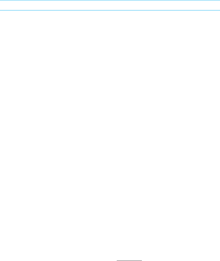
The raw data from these tests are presented in Figure 11.5. We show the number
of comparisons made and the number of swaps for each of the four sorting methods
on our six (ostensibly) random data sets.
Bubblesort Insertionsort
Data Comps Swaps Comps Swaps
127 8,001 4,024 4,146 4,024
511 130,305 64,184 64,690 64,184
2,047 2,094,081 1,058,276 1,060,314 1,058,276
8,191 33,542,145 16,804,307 16,812,488 16,804,307
32,767 536,821,761 268,317,072 268,349,824 268,317,072
131,071 8,589,737,985 4,054,936,240 4,296,967,076 4,296,836,017
Heapsort Quicksort
Data Comps Swaps Comps Swaps
127 1,423 836 930 215
511 7,826 4,416 4,883 1,100
2,047 39,431 21,707 24,596 5,430
8,191 190,910 103,572 121,762 25,365
32,767 894,810 479,714 594,064 116,024
131,071 4,103,982 2,181,680 2,665,459 523,552
FIGURE 11.5 Raw counts of comparisons and swaps.
We have theorems that claim that the worst-case running times for these four
sorts are O(N
2
)andO(N lg N). If our “random” data produced running times like
1
Our generation method would almost certainly not hold up under a rigorous test of random-
nicity, but we believe it is sufficient for this illustrative purpose.

268 CHAPTER 11 SORTING
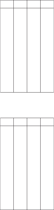
Bubblesort/N
2
Insertionsort/N
2
Data Comps Swaps Comps Swaps
127 0.496 0.249 0.257 0.249
511 0.499 0.246 0.248 0.246
2,047 0.500 0.253 0.253 0.253
8,191 0.500 0.250 0.251 0.250
32,767 0.500 0.250 0.250 0.250
131,071 0.500 0.236 0.250 0.250
Heapsort/(N lg N) Quicksort/(N lg N)
Data Comps Swaps Comps Swaps
127 1.601 0.941 1.046 0.242
511 1.702 0.960 1.062 0.239
2,047 1.751 0.964 1.092 0.241
8,191 1.793 0.973 1.143 0.238
32,767 1.821 0.976 1.209 0.236
131,071 1.842 0.979 1.196 0.235
FIGURE 11.6 Normalized counts of comparisons and swaps.
127 511 2,047 8,191 32,767 131,0710.0
0.2
0.4
0.6
0.8
1.0
1.2
1.4
1.6
1.8
2.0
Bubblesort
comps/N
2
Insertionsort
comps/N
2
Heapsort
comps/(N lg N)
Quicksort
comps/(N lg N)
FIGURE 11.7 Comparison counts for the four sorting algorithms.

11.11 Auxiliary Space and Implementation Issues 269
this, then we would have some reason to believe (but not a proof) that perhaps
these are not just worst-case running times but also average-case running times.
In fact, that’s exactly what we see. In Figure 11.6 we divide these counts by
N
2
and by N lg N as appropriate so as to estimate the constant C in the asymp-
totic estimate. The data of Figure 11.6 is graphed in Figure 11.7. It is reassuring
to notice that as the data size increases, the “constant” is in fact reasonably con-
stant, although there is some upward creep in both heapsort and quicksort. Our
earlier estimate was that heapsort as we implemented it would require 2N lg N
comparisons, so we would expect the constant to stabilize at no larger than 2.0.
One obvious observation is that quicksort is indeed faster than heapsort on this
(allegedly) random data. In addition to the implementation advantage that quick-
sort has, it would appear that on random data it also has an asymptotic advantage
as well. If we accept the truth of Theorem 11.1, we should not be surprised at
the graph for quicksort, but it’s nonetheless reassuring to have observations fit
the theory.
11.11 Auxiliary Space and Implementation Issues
When analyzing a sorting algorithm, the most prominent issue is the asymptotic
running time. In theory, this is the most important aspect of a choice of sorting
methods. Asymptotic running time, however, is not the only criterion to be consid-
ered. Indeed, if one is actually going to be sorting data,
2
then all of the real-world
considerations and characteristics of the problem to be solved must be brought into
the discussion. The U.S. Internal Revenue Service, for example, has a very different
problem when sorting some 200 million tax records that live on disk than does an
Internet server that has to take in packets in real time and sort all the packets for a
particular transmission in order to deliver them to the eventual recipient. We don’t
expect the IRS to be sorting constantly, but when it does it will sort a large number
of items. The packet server, in contrast, is sorting a small number of items, but it’s
doing a new sort on a new message all the time.
Further, data that is known to be almost sorted apriorishould probably be
sorted differently from data about which nothing is known. Data to be sorted on a
large mainframe might well be sorted differently from data on a desktop or laptop.
Unless one is an algorithmist or theoretical computer scientist, the goal in imple-
menting a sorting algorithm is probably to be able to sort data, and the real world,
however messy, must intrude.
2
As opposed to proving theorems about how one might sort data

270 CHAPTER 11 SORTING
11.11.1 Space Considerations
The first implementation issue to be considered is whether extra space is needed for
the sorting algorithm. In the case of bubblesort, insertionsort, heapsort, and quick-
sort, no extra space is needed other than the one extra location necessary for tempo-
rary storage in doing a swap of two records. The array in which the data are stored
at the beginning of the sort is the array in which the data are stored at the end.
In the case of mergesort, extra space is required, and the amount of extra space is
O(N), equal to the size of the original array. On the one hand, this is a major burden
on mergesort if all the data must be kept in memory. On the other hand, mergesort is
the one sorting algorithm, of the several we have discussed, that is highly suitable for
disk-to-disk sorting of very large files. One characteristic of mergesort that is highly
desirable for this purpose is that all the data are accessed in a purely sequential
way. Two (large) files are brought in from disk sequentially for comparisons and
the result array is written exactly in sequence to the output file. Since a disk is
at its best when streaming data to the processor, this match between best use of
the hardware and the needs of the sorting algorithm make mergesort a favorite for
large-file sorts. This is in sharp contrast to heapsort, whose access pattern goes all
over the array, pulling up entries n,2n,and2n + 1 that will be located in very
different places on disk. Even quicksort is likely to perform poorly in a disk-to-disk
implementation because it requires accessing and then rewriting (or not) at specific
locations that may or may not be contiguous on disk.
11.11.2 Memory
Of the three O(N lg N) sorting algorithms we have discussed—mergesort, heapsort,
and quicksort—we can generally decide that mergesort is not the best general-
purpose sort because it requires O(N) extra space. Between heapsort with guaran-
teed O(N lg N) running time and quicksort that is only guaranteed on average to
run in O(N lg N) time, it is somewhat surprising at first that quicksort has become
the standard sort found in software libraries, but that is in fact true.
Part of the reason for quicksort’s success is that the memory access patterns for
quicksort are far superior than those for heapsort given the constraints of standard
computer architectures. We normally only care about the running time of sorts when
we have large arrays to sort, so we assume, in dealing with real-world constraints,
that substantial memory space is needed for our array. The feature of quicksort
that makes it superior to heapsort for general applications is that quicksort usually
runs largely in cache, not in main memory.
Cache, which these days is usually on the processor chip, is a smaller, inter-
mediate memory space between the processor’s registers and logic units and the
RAM that lives elsewhere on the motherboard. For various reasons including the

11.11 Auxiliary Space and Implementation Issues 271
fact that cache is actually on the processor chip, access to cache is much faster
than access to main memory. This comes at a price in real dollars, though, and
while many desktops are configured with some number of gigabytes of RAM, cache
is still measured in megabytes, with as much as 8 MB showing up only in current
high-end processors. For the most part below the level that any programmer can
control (even in assembly language), the processor loads blocks of data from the
main memory RAM into the cache either as the data is requested or in anticipation
of requests for the data. As long as the processor’s requests for data can be met
with values from cache instead of main memory, execution is faster.
It is here, with respect to cache, that heapsort’s memory access patterns work
against the algorithm. Records accessed at subscripts n,2n,and2n + 1 are likely
to be in different blocks of memory for large values of n, so they are unlikely to be
in cache because they are only accessed once every so often. In contrast, quicksort
accesses sequential locations in the array with its moving pointers, and it rapidly
recurses down to working on subarrays that will fit in cache. Once the subarray fits
entirely in cache, all the processing can be done by moving data in cache, not in
main memory, with a concomitant increase in speed.
11.11.3 Multilevel Sorts
It is not uncommon for a large general-purpose sort to be implemented as a mul-
tilevel sort with more than one sorting method. Although a mergesort is effective
on large files, its effectiveness is greater in the later phases when merging large,
sorted arrays than in the early phases. One might well implement a sort of large
data by first bringing into memory blocks of data in as large a block as would fit
conveniently and efficiently, sorting that data in memory with a quicksort, and then
writing that block of data back out to disk. By doing this subsorting in memory,
one gets the advantage of a (faster) memory-based sort on blocks of data as large
as can be managed, and one can follow this with a disk-to-disk merge of the large
blocks of sorted data.
We will see a variation of this idea later in this chapter when we discuss sorting
on parallel computers.
11.11.4 Stability
A final consideration for sorting data is that some sorting methods are stable and
some are not stable. A sort is stable if two records that have the same key end up
being stored in the sorted array in the same order in which they are presented in the
original array. If record i precedes record j in the original array, and if both records
have the same key, then record i should still precede record j when the array is
eventually sorted. Stability of sorting algorithms is important, for example, when
one is adding new data to an already sorted list or when one is sorting on multiple

272 CHAPTER 11 SORTING
keys. If one is sorting on last name and is adding data to an existing list, one usually
wants the new data simply inserted where it ought to go in the augmented list. It
could be especially annoying to find that the original list of last name “Smith”
entries came out in a different order from what they had been before just because
a new “Smith” entry was added.
Not all sorts are stable. Heapsort, for example, is pretty much guaranteed not to
be stable. Bubblesort and insertionsort are stable provided one gets the “less-than”
and “less-than-or-equal” comparisons done properly. In the preceding implementa-
tion, two records are swapped if the key of one is greater than the key of the other.
If the keys are equal, the records are not swapped, so records of equal key end up
being stored in their original order, and the sort is stable. If one wrote the sort
comparison as if(key[i] >= key[j]), the records would still end up sorted, but
the sort would not be stable.
Quicksort is stable in the same way that bubblesort and insertionsort are stable,
that is, provided one takes care not to force the exchange of records with equal keys.
In all three instances we are moving records only because they are out of order,
and we do not move records that are locally in the correct order.
11.12 The Asymptotics of Sorting
We have seen three sorting algorithms that run in O(N lg N) time. What we will
now prove is that this is asymptotically the fastest possible running time for any
sorting algorithm that sorts by comparing keys. This is a very important result. If
the asymptotic running time of heapsort, mergesort, and quicksort (and any other
sort we can come up with that has this running time) is as good as is possible, then
the best we can do is to improve the constant out front and to improve the imple-
mentation; no further theoretical improvement is possible. As we have seen from
Figures 11.5 and 11.6, quicksort appears to have a better constant than heapsort, at
least on our experimental data. As we have discussed previously, it also has better
characteristics when implemented on modern computers. Any algorithm that would
replace quicksort as the standard would have to have an O(N lg N) running time
and a better constant on observed execution instances or better implementation
characteristics.
11.12.1 Lower Bounds on Sorting
What we are going to prove in the next few pages is a lower bound on the cost of sort-
ing by comparisons. That lower bound will be O(N lg N). Since that is the worst-case
running time for heapsort and mergesort, we can conclude that no sorting algo-
rithm that uses comparisons will be asymptotically faster than either of these. If one

11.12 The Asymptotics of Sorting 273
algorithm is to be faster than another, it will be either because the constant out front
is smaller (remember Figure 6.1) or because the algorithm just happens to be better
suited to the way certain computers (possibly most computers) are constructed.
Consider an algorithm to sort three elements {a, b, c} by comparison of keys as a
decision tree, as in Figure 11.8. What we are going to do is show that there is a lower
bound on the number of comparisons needed to sort by comparisons. Specifically,
we will show that no comparison-based sort can possibly sort all possible input
permutations in fewer than O(N lg N) comparisons.
?
?
b < c
a < c
a < b
a < c
b < c
?
a, b,c
Y
a, c,b
N
Y
c, a,b
N
Y
?
b, a,c
Y
?
b, c,a
Y
c, b,a
N
N
N
FIGURE 11.8 A decision tree.
What we have in the decision tree is a tree of comparisons to be applied in order
going down from the root, so that after the sequence of comparisons down any given
path, we know that the leaf provides the order of the input data.
For example, for three inputs {a, b, c}, with the six possible ways in which those
values could appear in sorted order, we could first compare a against b.Ifa is less
than b, then we have one of the three orders a<b<c, a<c<b,orc<a<b.And
that’s all we know after that one comparison. If we next compare a against c,and
find that a is in fact less than c, we can exclude the case c<a<band we know
we have one of the two possibilities a<b<cor a<c<b.Athirdcomparisonof
b against c is necessary to resolve this uncertainty.
If we can prove a lower bound for sorting using decision trees, then clearly the
number of levels in the tree is that lower bound because each level corresponds to
one comparison. We point out that there are many decision trees, all of which result
in being able to uniquely identify which correct sorted order is found in the data.
If we are to prove a lower bound, we have to show that no decision tree has fewer
than some minimum number of levels.
Let’s just hammer away with what we know:
• There are N! total permutations of N elements, so a decision tree for sorting
N elements must have at least N! leaves. If we don’t have a path from the root

274 CHAPTER 11 SORTING
(the first comparison) down to every possible input permutation, then we can’t
actually sort.
• For a binary tree of k leaves and height h,wehavek ≤ 2
h
,thatis,h ≥ lg k.
• Thus a decision tree with N! leaves must have height at least lg(N!).
• The lower bound for number of comparisons is the lower bound for the height
of the decision tree.
• So the lower bound for sorting by comparing keys is lg(N!).
It may take a moment to understand why this guarantees a lower bound and not
just a lower bound for this instance or this representation of the problem. We have
chosen to compare a with b in the top level, and then made other choices as well.
If we chose to compare a with c at the top level, we could produce a decision tree
that was merely the result of exchanging b for c throughout the tree. Any other
decision tree is merely the result of permuting the input of the three elements a, b,
and c, not a change to the algorithm itself.
Next, we can observe that all these comparisons are necessary. With each com-
parison, we have a set of possible permutations for either of the two outcomes of the
comparison. If we take the right path for the first two levels, we know that a is not
less than b and that a is not less than c. We have at this point no information as to
the relative position of b and c.Bothb ≤ c ≤ a and c ≤ b ≤ a are possible, and since
this is a sorting algorithm, any possible ordering of the three inputs is a possible
input to the algorithm. Unless and until we compare b against c, we cannot deter-
mine which of the two remaining possibilities is correct. Unless we have a decision
tree with at least as many leaves as there are possible input possibilities, we will
not have a path of decisions that will uniquely identify each of the possible inputs.
11.12.2 A Proof of Lower Bounds
We now know that it takes at least O(lg(N!)) comparisons to sort N items. The
question is, exactly how big is lg(N!)? The answer, at least for today’s purposes,
comes from Stirling’s formula that we introduced in Chapter 6.
Theorem 11.2
Sorting N items by comparisons takes at least O(N lg N) comparisons.
Proof By what we have just done in the preceding section, what we need to show
is that
lg(N!) = O(N lg N).

11.12 The Asymptotics of Sorting 275
From Stirling’s formula we have
N!=
√
2πN
N
e
N
e
α
N
.
This means that
lg(N!) =
1
2
(1 + lg π +lgN)+N(lg N − lg e)+α
N
lg e
= N lg N − N lg e +
1
2
(1 + lg π +lgN)+α
N
lg e
≥ N lg N − N lg e
≥
1
2
N lg N (for large N)
= O(N lg N)
comparisons are needed to sort N items for large N. The first line becomes the
second line by simply rearranging terms; the second line becomes the third because
we are throwing away terms that are known to be positive; and the final inequality
holds because we know that N lg e = o(N lg N), so for large N we have N lg e ≤
N lg N
2
, and the inequality holds. Sorting cannot be done in fewer than O(N lg N)
comparisons.
11.12.3 Lower Bounds for the Average Case
We have shown that the lower bound for sorting is O(N lg N) by showing that in
the worst case the maximal path down a decision tree has a path of length at
least lg(N!). We can actually prove something somewhat stronger, which is that
the average path length down the decision tree must be at least of length lg(N!).
What we can conclude from this is that we don’t have pathological worst cases that
might be few and far between. Quite the contrary, if we have best cases that take
less time, it is the best cases that are exceptional and few and far between.
Consider the general decision tree for sorting N items. The tree has N!leaves,
so the average path length from the root to a leaf is
sum of all path lengths to leaves
N!
.
We start with a lemma about the numerator.
Lemma 11.3
The sum of all path lengths to leaves is minimized when the tree is completely
balanced.

276 CHAPTER 11 SORTING
Proof If we disconnect any subtree from a balanced binary tree and move that
subtree so as to connect it somewhere else in a binary tree, we necessarily have
increased the sum of the path lengths.
We can now prove the theorem.
Theorem 11.4
The average case of any sort by comparison of keys is at least
lg(N!)
comparisons.
Proof The minimal sum of all path lengths to trees is
(N!) ·(lg(N!))
so the average path length is bounded below by lg(N!).
Thus, sorting either in the worst case or in the average case takes at least
O(N lg N) comparisons. What this means is that we cannot improve upon sorting
methods such as heapsort and mergesort in the worst case, and we cannot improve
upon heapsort, mergesort, or quicksort in the average case.
11.13 Sorting in Parallel
We will close this chapter with a section on parallel computing, specifically on
how to sort on a distributed memory parallel machine. The canonical version
of a distributed memory parallel computer is a collection of standard computers
connected by as fast an interconnect as one can afford. This is the model of
computation adopted by the very common Beowulf cluster computers. Each node
is an independent computer and can only access its own memory locations. If
processor A wants to get data stored in the memory of processor B, for example,
then A must send a message to B requesting data, and B must respond by sending
back the data in another message. This makes the communication of data the
bottleneck to efficient computation because the overhead of sending a message
across a slow connection (possibly just Ethernet) is very large when compared
with the cost of accessing a memory location local to the computer.

11.13 Sorting in Parallel 277
In a cluster computer, a head node computer farms out identical tasks to a
collection of compute nodes, each of which is an independent computer. The com-
pute nodes process for as long as they can using the data they have available to
them locally. At some point in the computation, the compute nodes will probably
have to exchange data. In the cheapest version of a Beowulf cluster, the inter-
connect would be simply an Ethernet connection; although faster interconnects
exist, they are still much slower than is a simple memory reference local to the
computer itself.
Invariably, it is this communication of data from one processor to another that is
the bottleneck that slows down the parallel computation. In the worst-case scenario,
if one processor is collecting data from all the other processors, then the incom-
ing data flood will overwhelm the bandwidth. Ideally, when we have to exchange
data, we would like to arrange things so that all processors are sending and receiv-
ing equal amounts of data because this will distribute the data equally across the
communication paths.
We note that the other kind of parallel computer is a shared memory parallel
computer in which all processors have access to all memory locations in the machine.
Clearly, this is a more powerful model of computation because it eliminates the need
for moving large quantities of data from one machine to another. However, this
power comes at a price—it is not unreasonable for the switch between processors
and memory to be the most expensive single part of the computer. It just isn’t
very easy to have lots of processors all with the ability to access huge amounts of
memory at the very high speeds and very fine granularity of loading and storing
entries in memory.
The contrast between the two different kinds of parallel computer is made very
clear when considering how to sort. Let’s consider what happens when we use four
processors labeled P
0
through P
3
to sort 32 integers, and assume that the data
is initially distributed as shown in Figure 11.9. Remember that computation by a
P
0
P
1
P
2
P
3
25 27 26 3
29 4 24 5
7 8 19 9
2 1 2 2
10 3 12 13
15 14 5 4
18 21 20 3
22 30 28 31
FIGURE 11.9 Initial configuration of data for a parallel sort.

278 CHAPTER 11 SORTING
processor on its own memory locations is fast, but communication of data from one
processor to another is slow.
The first step in the parallel sorting process is for each processor to sort its
own data, using whatever is the fastest sort for that processor. (Probably this is a
quicksort.) This results in the data shown in Figure 11.10.
P
0
P
1
P
2
P
3
2 1 2 2
7 3 5 3
10 4 12 3
15 8 19 4
18 14 20 5
22 21 24 9
25 27 26 13
29 30 28 31
FIGURE 11.10 Data after the local sort.
Now the problem is to extract the sorted lists from the processors and merge
them together to create a single completely sorted list. So far, our computation
has resembled a mergesort, and if this were a single processor doing a mergesort
on disk, we would just continue with the merge. But the rules are different with
parallel machines, especially with Beowulf clusters. The overhead cost of the head
node’s sending messages to P
0
and P
1
, say, asking for the top two elements and
merging the two, is very high. If we are going to send messages and move data,
we want to move blocks of data; we absolutely do not want to pull off entries from
each processor one at a time. Further, if the head node is performing a merge from
P
0
and P
1
, then P
2
and P
3
are sitting idle, and we don’t want half of the machine
doing nothing; we want all processors working in parallel as much as possible. Note
that if we had a truly shared memory machine, then this would be a simple task
even in parallel; although there can be some contention in the lower levels of the
hardware by having multiple processors reading from the same hardware memory
banks, there is nothing algorithmic that prevents all processors in a shared memory
computer from reading different locations in memory simultaneously.
The solution is as follows. Given that we have n = 4 processors, we let each
processor select the n − 1 = 3 breakpoint elements that break up local memory into
four pieces. In Figure 11.11, we read the boldface numbers to mean, for example,
that entries for processor P
2
that are less than or equal to 5 are in the first quarter,
entries greater than 5 but less than or equal to 19 are in the second quarter, and
so forth.
11.13 Sorting in Parallel 279
P
0
P
1
P
2
P
3
2 1 2 2
7 3 5 3
10 4 12 3
15 8 19 4
18 14 20 5
22 21 24 9
25 27 26 13
29 30 28 31
FIGURE 11.11 Data after determining local breakpoints.
Each processor now sends its samples to the head node, so the head node has
the data in Figure 11.12.
7 15 22 3 8 21 5 19 24 3 4 9
FIGURE 11.12 Head node sample data before sorting.
The head node now sorts these sampled values, and then it splits its sample data
into four quarters, as indicated by the bold entries in Figure 11.13.
3 3
4
5 7
8
9 15
19
21 22 24
FIGURE 11.13 Head node sample data after sorting.
The head node now broadcasts the boldface sample values (4, 8, and 19) to all
processors. Each processor now sends all entries less than or equal to 4 to processor
P
0
, all entries greater than 4 but less than or equal to 8 to processor P
1
, all entries
greater than 8 but less than or equal to 19 to processor P
2
, and all entries greater
than 19 to processor P
3
. This results in the situation illustrated in Figure 11.14. In
this tableau we have listed the “local” data first and then the entries that would
have been received in processor subscript order, but this is arbitrary, since we cannot
usually rely on a cluster computer to send data in predictable ways. For example,
for P
3
, the entry 31 comes from the processor locally, the entries 22, 25, and 29
come from P
0
, the entries 21, 27, and 30 come from P
1
, and the entries 20, 24, 26,
and 28 come from P
2
.
Now, each processor sorts its own data locally, using whatever is its fastest sorting
algorithm, to produce the final tableau in Figure 11.15.

280 CHAPTER 11 SORTING
P
0
P
1
P
2
P
3
2 8 12 31
1 7 19 22
3 5 10 25
4 5 15 29
2 18 21
2 14 27
3 9 30
3 13 20
4 24
26
28
FIGURE 11.14 Data after the global sends.
P
0
P
1
P
2
P
0
1 5 9 20
2 5 10 21
2 7 12 22
2 8 13 24
3 14 25
3 15 26
3 18 27
4 19 28
4 29
30
31
FIGURE 11.15 Final tableau of data.
We can now stream the data in sorted order to the head node in processor
subscript order.
11.13.1 Analysis
Let’s step back a moment and think about what we have done, what will make this
algorithm work, and why this is a better approach than other ideas for sorting on
distributed memory computers.
First, we have been able to use the parallelism of the computer. Except for the
time spent by the head node in sorting the samples, all the processors were working
and were working in parallel. That’s a good thing.

11.13 Sorting in Parallel 281
Second, the time spent by the head node in sorting, when the other processors
are sitting idle, is probably relatively short. Each of n processors sends n −1val-
ues to the head node. For a 1024-processor machine (which is large but not huge),
this results in the head node’s having to sort about a million items. Given that
each compute node probably had gigabytes of storage, each local node was prob-
ably sorting much more than a million items, so the head node’s sort is small by
comparison.
The third consideration is the data movement. If there were n processors, then
each processor had to send nearly all its data to other processors, so in essence we
were moving all the data exactly once. But we were moving all the data simultane-
ously to all the other processors. We can’t do much about the fact that the overall
network might have been bandwidth limited, but we didn’t create any hot spots by
moving all the data on a single wire to a single machine.
Finally, let’s think about whether this actually works in practice. If the data get
distributed randomly to the various processors, then each processor’s data will be
similar. This means the breakpoints sent to the head node will be similar. When
the head node sorts to produce a set of global breakpoints, these breakpoints sent
back to the local processors will be fairly similar to what the local processors
already had. This means that we will in fact be sending about 1/nth of the data to
each of the other processors, thus balancing the load on the network. There will be
some imbalance in the size (look again at Figure 11.15, in which P
1
is underloaded
and P
3
is overloaded), but it ought not to be too bad if the data are essentially
randomly distributed.
Contrast this with the worst-case situation (at least for the load balancing of the
data movement) in which the data are already sorted when they get distributed to
the local processors, but the distribution is in reverse order. If the original configura-
tion, for example, is as in Figure 11.16, then each processor winds up having to send
all its data to a single other processor, and there is no real balancing of the load.
P
0
P
1
P
2
P
3
25 17 9 1
26 18 10 2
27 19 11 3
28 20 12 4
29 21 13 5
30 22 14 6
31 23 15 7
32 24 16 8
FIGURE 11.16 Worst-case parallel sort tableau.

282 CHAPTER 11 SORTING
In general, sorting is the worst possible kind of computation to be done on a
parallel machine. No matter where we initially place a data element on a local
processor, there is some input data set that would require the element eventually
to wind up at any other processor. In many parallel computations in physics, for
example, there is a known locality of reference. Seattle’s weather, for example,
has little effect on Miami, so one can safely task one processor with computing
Seattle weather and one with computing Miami weather and not expect there to be
much data movement between the two. But in sorting, all possible configurations
could happen, This makes controlling the worst case of data movement the primary
problem for a cluster computation.
As a general rule, the methodology used in this parallel sorting algorithm is the
norm for cluster computing. If we cannot aprioriforce data and computation to
be localized, then we rely on statistics to try to balance the load. If we suspect that
our data might already be partially sorted, then we would not choose to pivot in a
quicksort on the last element in the array but would instead do a quick sampling
of the array to pick a value we hope would be closer to the middle. Similarly, we
sample locally in this parallel sort and then sort the samples, in hopes of producing
global breakpoints that will break the entire data set into equal-sized chunks. If we
cannot rely on deterministic predictions of what the data will look like, then we
must rely on statistical analysis and hope for reasonably random inputs.
11.14 Summary
We have in this chapter provided a thorough introduction to the standard sort-
ing algorithms of bubblesort, heapsort, insertionsort, mergesort, and quicksort. We
have done both a worst-case running time analysis and an average-case running
time analysis of these algorithms, and discussed the nature of average-case analysis
compared to the (usually easier) worst-case analysis.
Having done an asymptotic analysis, we have gone further to consider the prac-
tical aspects of sorting, such as the use of auxiliary space, disk-based sorting for
very large data sets, the extent to which the input data is already sorted, multi-
level sorting, and stability. These considerations often affect the choice of a sorting
algorithm other than the theoretically best algorithm. Indeed, the common use of
quicksort as the default algorithm is not because its worst-case running time is opti-
mal, but because its average-case running time is O(N lg N), the pathological cases
seem very rare, and it can be implemented more efficiently on modern computers
than the worst-case asymptotically better heapsort algorithm.
Finally, in a starred section, we have discussed sorting on a distributed memory
parallel computer. This is an example of the use of the assumption of statistically
random data in an algorithm that can be shown to be efficient if that assumption
holds.

11.15 Exercises 283
11.15 Exercises
1. Given the following sequence of integers, show the first three levels of the
mergesort from the bottom up (that is, first comparing adjacent pairs).
33, 55, 2, 19, 92, 18, 45, 74, 88, 27, 51, 6, 91, 22, 44, 13
2. If we choose the last element in the (sub)array as the pivot element, show
the first two complete phases of quicksort. The first phase should use the last
element as the pivot and result in two subarrays. The second phase should use
the last element in each subarray as the pivot and result in four subarrays.
33, 55, 2, 19, 92, 18, 45, 74, 88, 27, 51, 6, 91, 22, 44, 13
3. Repeat the previous exercise but choose the first element as the pivot instead
of the last.
4. In the best possible case, what is the minimum number of comparisons neces-
sary in order to determine the proper order of n integers?
What does this tell you about the minimum distance from the root to a leaf
in a decision tree for sorting?
5. Consider the possible input sequence of data items:
Freshman Tyrone
Sophomore Tyrone
Freshman Amanda
Sophomore Amanda
We would like this to be sorted first by class, then by name, so our desired
output is
Freshman Amanda
Freshman Tyrone
Sophomore Amanda
Sophomore Tyrone
We have said that our bubblesort as written is stable with the strict “greater
than” of Figure 11.1, and we have said that stability of sorting is important
when one is doing a multilevel sort first on one key, then on a second key.
With the strict >, we pull the first occurrence of the least value to the top; if
we wrote ≥ instead of >, we would pull the
last occurrence of the least value
to the top.

284 CHAPTER 11 SORTING
Trace the execution of a bubblesort with ≥ replacing the >, sorting first on
class (freshman is lower, of course) and then alphabetically on name. Demon-
strate that we don’t get a stable sort by showing that we don’t get what we
want as the output.
(In the case of bubblesort, we write > more naturally because there is no
reason to do the extra work of an exchange for an equal key. In the case of
heapsort, for example, it is not at all obvious how we might be able to force
stability.)
6. In the preceding problem, we sorted first on class and then on name. Some
people might have argued that it would be easier to concatenate class and
name and do a single sort.
Under what circumstances might this not be such a simple thing to do
or perhaps not a desirable thing to do? (Hint: think Java, object-oriented
programming, reusable code, etc.)
7. The table in Figure 11.6 suggests that our insertionsort takes about 0.25N
2
comparisons and our quicksort takes about 1.1N lg N comparisons for small
N. If we accept these constants as the actual values, how large does N have
to be for quicksort to take fewer comparisons? Given that quicksort is a more
complicated program, does this suggest that we should switch to insertionsort
when the subarrays in quicksort get sufficiently small?
8. Implement a complete mergesort from the bottom up. Include with your sorted
output a counter of the number of comparisons.
9. Implement a complete mergesort recursively from the top down. Include with
your sorted output a counter of the number of comparisons.
10. Implement a complete quicksort as a recursive computation. Make sure that
you do not create new arrays and thus waste memory but rather are working
on subscripts pointing into an array that is declared as an instance variable
for the class. Include with your sorted output a counter of the number of
comparisons and compare this to Figure 11.6.
11. Implement quicksort, but this time, if the subarray is of length at least 9,
sample the first element, the last element, and the middle element, and choose
the middle value as the pivot. Count the comparisons and see if you do any
better than either your previous implementation or Figure 11.6. (Don’t worry
too much about rounding up or down for the pivot or about rounding up or
down to get the middle subscript. Statistically this shouldn’t matter, although
you might see if it does on the sample data you use.)
12. Implement a sort on an ArrayList of Record instances (from Figure 3.1) that
will allow you to sort either by name, by course being taught, or by office

11.15 Exercises 285
number. The office number is formatted with the leading character as the
floor number, the second as the building wing, and then the room number,
and you want to sort by floor, then by wing, then by number. Use an interface
to allow a comparison method to accept as parameters both a Record value
and a constant to direct which field is to be used for sorting.

..................Content has been hidden....................
You can't read the all page of ebook, please click here login for view all page.