10
Why Is Time Variance Difficult?
In my previous book, Building and Maintaining a Data Warehouse, I demonstrated how to build time variance into a data warehouse. In that discussion, an object in a row of a fact table joins to a dimension table via a primary key/foreign key join with an additional WHERE clause that selects the one row of the dimension table that has the Effective and Termination Dates that form a time interval that surrounds the date of the transaction in the fact table row (Silvers 2008). This and subsequent chapters constitute both a retraction and a correction of that time variant design. In practice, I have found that this model performs well at low cardinalities of data. I found that as long as the number of fact table rows is small, the number of objects joining to dimensions is small, and the number of dimension rows is small, the time variant design in Chapter 5 of Building and Maintaining a Data Warehouse performs satisfactorily well. If, however, any of those points of cardinality (i.e., number of fact table rows, number of objects, number of dimension table rows) increases moderately, the query performance of the data warehouse becomes less and less satisfactory as the cardinality increases. When any of those points of cardinality increases significantly, the data warehouse simply ceases to perform well at all. This conundrum was the genesis for the time variant solution design outlined in Chapter 11, “Time Variant Solution Definition.”
Relational Set Logic
SQL queries retrieve data in sets of rows. A basic SQL query (SELECT * FROM TABLE) shows that the statement is asking for all the rows in a table. All the rows constitute a set, specifically a set of rows. The RDBMS retrieves all the rows from the table and delivers them to the user. If a query selects data from two tables, then it retrieves two sets of rows as it builds the final result set. If a query retrieves data from three tables, then it retrieves three sets of rows as it builds the final result set. If a table has an index on a column, and a query uses a WHERE clause on the specific column, the RDBMS will use the index to retrieve only the subset of rows that match the WHERE clause in the query as it builds the final result set. That subset of rows is still a set of rows. So, no matter how you write the query or index the tables, the RDBMS will always retrieve data in sets of rows. This is the set logic inherent in every RDBMS.
Set logic is a very powerful tool and an innovative leap forward past the flat file and hierarchical databases that preceded relational data structures. Prior to relational data structures, data was stored in flat files or keyed files. A procedural application was required to retrieve data from these files and databases. A business user could not submit an ad hoc query against a flat file, join that with a keyed file, and then join the result set of those two files with another keyed file. Prior to relational data structures, that technology did not exist. That technology is the relational data structures of an RDBMS. So, the set logic of an RDBMS is not a weakness. Rather, it is an innovative leap forward that suddenly made large volumes of data available to business users. Instead of waiting for an application to run a job that would create a file that was a combination of the data in two separate files, the creation of an RDBMS gave business users the ability to retrieve the data they need without waiting for a job to run a program that reads the files, combines their data, and then writes a file.
Set logic give an RDBMS the ability to manipulate large volumes of data, join separate sets of data, and combine their data into a single result set without a job running a program that generates a file. Instead, the business user submits a query and the RDBMS does all the work. When the RDBMS is finished, it passes the result set to the business user who submitted the query. For that reason, set logic is the strength of every RDBMS.
Sets—The Bane of Time Variance
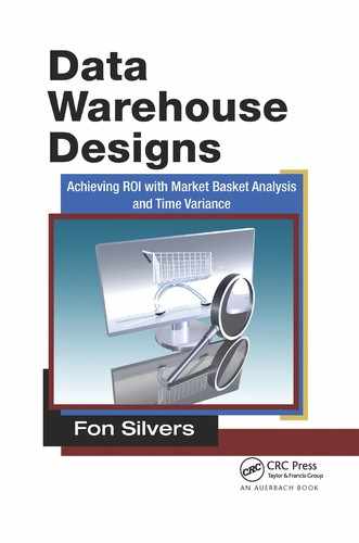
Set logic, the strength of every RDBMS, is the bane of Time Variant data. The problem is the set of rows. All the millions of occurrences of a transaction are represented by millions of rows in a fact table. Each of those millions of rows in the fact table reference an object (probably multiple objects) in a dimension table. An attribute of an object may be prone to occasional changes. Each of those iterations of the object is represented by a row in the dimension table. Each of those dimension rows uses the Row_First_Date and Row_Last_Date columns to indicate the boundaries of the interval of time during which the data in that dimension row was in effect. Each individual row of those millions of rows of the fact table will ultimately join to only one dimension row, specifically the dimension row that was in effect at the time of the transaction represented by the fact row. However, because the RDBMS retrieves data in sets of rows, the fact table actually is joining to all the rows in the dimension table. After the join between the fact and dimension table(s) is complete, then the rows that do not match the time variant condition (i.e., Transaction Date between the Row_First_Date and Row_Last_Date) are discarded. Unfortunately, those rows had to be gathered in memory before they could be discarded. A more efficient path would be to never have gathered the rows that do not meet the time variant condition.
The example in Figure 10.1 shows that a transaction occurred on March 11, 2005. The object of that transaction has an Item Key equal to the number 4. The Transaction table on the left has one row that represents that transaction. When joining to the Item dimension table on the right, the Item Key equal to 4 joins to all the rows in the Item dimension table with an Item Key equal to 4. Then, the RDBMS inspects the set of rows that have an Item Key equal to 4, searching for the row with a time bounded by the Row_First_Date and Row_Last_Date that encompasses the Event_Date from the Transaction fact row. The final result set includes the fourth row, wherein the attribute is yellow.
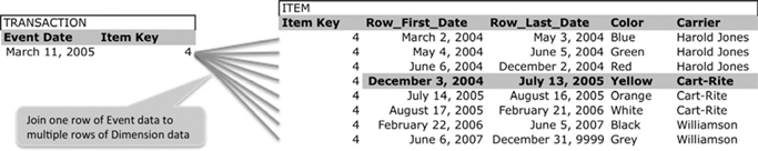
FIGURE 10.1
Time Variant set logic.
Why is the RDBMS unable to use an index or some other relational structure to join the Transaction fact table row to the one and only Item dimension table row that has an Item Key equal to 4 and was in effect on March 11, 2005? The reason is simple. No row in the Item dimension table has both the Item Key equal to 4 and the date March 11, 2005.
The example in Figure 10.1 is rather simple and small. The simplicity of that example is for introductory purposes only. Figure 10.2 extends this example to include Third Normal Form dimension tables that capture the Color Formula and Carrier Terms. Figure 10.2 shows that every row of the Item dimension table joins to every row of the Color Formula where the Color of the Item matches the Color of the Color Formula table. After each Item.Blue row joins to three Color_Formula.Blue rows, all but one row (Blue, C2387J, November 19, 2004, July 18, 2006) are discarded. After each Item.Green row joins to two Color_Formula.Green rows, all but one row (Green, UU879, February 13, 2002, July 13, 2005) are discarded. This same pattern repeats for the Red, Yellow, Orange, White, Black, and Grey colors.
The Carrier_Terms dimension table is a bit different from the Color_Formula table in that multiple Transaction rows have the same Carrier name. All the Item rows that have the Carrier equal to “Harold Jones” join to the Carrier_Terms dimension table where the Carrier name is Harold Jones. Only after all those joins have been performed does the data warehouse attempt to discard all but one row (e.g., Harold Jones, 14:14, December 16, 2004, July 4, 2006). This also happened for the Carriers Cart-Rite and Williamson. In each case, within the join of a foreign key to a primary key, that join becomes a product (or Cartesian) join. After all the rows have been joined, only then is the Time Variant logic of the dates performed.
The example in Figure 10.2 includes only one Transaction row, only one Item with multiple Type 2 Time Variant rows, and two dimension tables (Color Formula and Carrier Terms) that join to the Item dimension table. If the Color Formula or Carrier Terms table join to more dimension tables, the collection of product joins increases with each additional Type 2 Time Variant table. As the proliferation of transaction and dimension rows increases, the performance degradation also increases. As the proliferation of levels, or layers, of dimension tables increases, the performance degradation also increases. Before long, the proliferation of tables and rows causes the performance degradation to render the data warehouse unresponsive.
The join between a fact table row and a dimension table row would work much better if it were indeed a join between a single fact table row and a single dimension table row. Unfortunately, it is a join between a fact table row and a set of dimension table rows. Multiply that join, between a row of fact data and a set of rows of dimension data, by the number of fact rows; then, multiply that by the number of sets of dimension rows and you have a performance bottleneck on your hands. Relational data structures offer no way to index a table on dates between the Row_First_Date and Row_Last_Date because the date value between those two dates is not in the dimension table. An RDBMS cannot apply an index to data that is not there. As a result, Time Variant data, which sounds wonderful in a book or article, becomes a performance bottleneck early in the cardinality growth of the data warehouse.

FIGURE 10.2
Time variant set logic with dimensions.
Options
The search for a solution was initially guided by two questions: “What do I already possess that might solve the performance bottleneck?” and “What has someone else found that solves the performance bottleneck?” The first question led to the consideration of the RDBMS infrastructure. The stored procedure function within every RDBMS might be an option. The second question led to the discovery of temporal databases. In this context, temporal and time variant are synonymous. So, maybe someone else really did solve the performance bottleneck of Time Variant data.
Stored Procedures
Every generally available RDBMS offers the procedural functionality of a stored procedure that uses a cursor to fetch rows one at a time. That procedural cursor/fetch method works well for stored procedures because stored procedures are able to loop through millions of rows, one at a time, applying logic to each row individually. BI Reporting tools and individual data warehouse users rely on the RDBMS to perform the tasks defined in SQL queries. Unfortunately, the cursor/fetch method is not compatible with the SQL queries used by Business Intelligence Reporting (BI Reporting) tools, or the ad hoc queries written by individual data warehouse users.
If we were to use stored procedures to solve the performance bottleneck of Time Variant data, reports would be written as code in a stored procedure. A job would run the stored procedure, which could output its data in the form of a file or a table. This is eerily similar to the jobs and programs that retrieved data from flat files and keyed files prior to the advent of the RDBMS. This solution would not work for the same reason the programs that read flat files and keyed files were replaced by queries that retrieve data from one or more fact tables.
Temporal Databases
Another option is temporal databases. Temporal databases attempt to optimize the join between a fact row with a single event date and a dimension table with two date columns that form an interval (Date, Darwin, and Lorentzos 2003). That construct of a single date joining to an interval of dates is called a “tuple” (Clifford, Jajodia, and Snodgrass 1993; Date, Darwin, and Lorentzos 2003). Within the tuple construct are the two representations of time—Valid Time and Transaction Time. Valid Time is the moment or interval of time wherein the data in a row reflected the reality of the enterprise. Transaction Time is the moment or interval of time wherein a row of data was in effect. Valid Time refers to the data in the row and Transaction Time refers to the row (Clifford, Jajodia, and Snodgrass 1993; Date, Darwin, and Lorentzos 2003). The complexity of the tuple construct creates several relational integrity issues that require the enforcement of constraints by the RDBMS (Date, Darwin, and Lorentzos 2003; Gertz and Lipeck 1995).
The Tuple construct in the temporal database is not quite a Type 3 Time Variant data structure. A Tuple does not present alternate dimensions (e.g., 2001 Region, 2002 Region, 2003 Region) that exist next to the Type 1 or Type 2 Time Variant dimension value (e.g., Region). Instead, the Tuple offers multiple versions of an entity/attribute/property relationship. For example:
On May 14, 2003, the data warehouse recorded that the Color as of May 12, 2003, was blue.
On June 8, 2003, the data warehouse recorded that the Color as of May 12, 2003, was red.
On July 21, 2003, the data warehouse recorded that the Color as of May 12, 2003, was green.
On Nov. 11, 2003, the data warehouse recorded that the Color as of May 12, 2003, was white.
This has a double layered effect of Time Variance of the Time Variant data, which is not the alternate reality intended by Kimball’s Type 3 Time Variant design (Kimball 2005).
The query language for these temporal tables has not yet achieved a single standard query language. One query language uses Relation Variables (RelVars) (Date, Darwin, and Lorentzos 2003). Another query language in use with temporal databases is the Historical Query Language (HSQL) (Clifford, Jajodia, and Snodgrass 1993). A third temporal query language is the TSQL2 (Temporal SQL version 2) (Androutsopoulos, Ritchie, and Thanisch 1995; Bohlen, Jensen, and Snodgrass 1995). None of the query languages have been generally adopted. The difficulty of learning such a query syntax, lack of a standard, and lack of general adoption render the use of temporal databases rather difficult.
The relational integrity issues and relational integrity constraints work together to render the task of managing time variant data even more difficult than it was for a nontemporal RDBMS. The double layered (i.e., Valid Time & Transaction Time) Time Variant data can cause relational integrity issues that are prevented from occurring by constraints within the RDBMS (Gertz and Lipeck 1995).
The confusing query languages, none of which has yet been declared the standard, render the task of querying time variant data more difficult than it was for a nontemporal RDBMS. The tuple construct embraces the set logic inherent in an RDBMS, rather than resolve the set logic to join one row of fact data to one row of dimension data. For these reasons, a temporal database is not the solution to the performance bottleneck I was seeking.
Time Variant Solution Design
The set logic inherent in every RDBMS causes each row of a fact table to join to all the rows of a dimension table for a given primary key. The result of that is a significant performance bottleneck. Stored procedures can retrieve one row at a time but cannot be used by business users and BI Reporting tools to query data from a data warehouse. Finally, temporal databases are a collective set of efforts to reconcile the join issue in time variant data. In the process, temporal databases actually increase the workload on the RDBMS as it enforces relational integrity constraints to avoid relational integrity issues in the temporal database. The temporal query languages are confusing and, as yet, not standardized.
So, what is the solution? How can a data warehouse present time variant data without the performance bottleneck caused by set logic, without the relational integrity issues, and without the confusing query language? Chapter 11 will present a Time Variant solution design that resolves all these design issues and delivers Time Variant data.