
13
ETL into a Time Variant Data Warehouse
The purpose of an Extract, Transform, and Load (ETL) application is to bring data from the enterprise into a data warehouse. That may sound rather simplistic. However, the simplicity of that statement belies the complexities of ETL. In Building and Maintaining a Data Warehouse, Chapter 6 explains the analysis, architecture, design, development, and implementation of an ETL application. If you are reading this chapter intending to learn all you need to know about ETL, please refer to Chapter 6 of Building and Maintaining a Data Warehouse. For a data warehouse rookie, the text of that chapter will provide the foundation information necessary to understand and incorporate the Time Variant ETL design discussed in this chapter. The fundamental ETL concepts included in this chapter include Changed Data Capture (CDC) and ETL Key. The Time Variant ETL design will build on these two concepts.
Changed Data Capture
Entities
The CDC function applies specifically to dimension tables. Remember, dimension tables contain the entities of the enterprise. Those entities can include the products, locations, personnel, vendors, customers, formulas, transportation vehicles, and so on. Entities are those things that are somehow involved in the business processes of the enterprise. For example, the manufacture of a product might include the following entities:
Factory Worker: The person performing or monitoring the manufacture of a product
Raw Materials: The physical inputs into the manufacture process
Location: The factory in which the manufacture occurred
Formula: The algorithm by which raw materials are combined into a finished product
Each of those entities could be described, or further defined, by other entities:
Factory Worker: The person performing or monitoring the manufacture of a product
Certification: The jobs that a factory worker is educated to perform
Safety Rating: The safety risk level associated with a worker based on past history
Raw Materials: The physical inputs into the manufacture process
Supplier: The vendor who provided a raw material to the enterprise
Quality: The level of rejected raw materials associated with the Supplier and that specific raw material based on past history
Location: The factory in which the manufacture occurred
Geography: The physical region wherein the factory is located
Hierarchy: The organizational placement of the factory within the enterprise
Formula: The algorithm by which raw materials are combined into a finished product
Fail Rate: The percentage of rework associated with a specific formula
Skill Set: The abilities required to perform the manufacture process with a specific formula
Attributes
When an entity describes or defines another entity (e.g., Certification and Safety Rating describe Factory Worker), that describing and defining entity is an attribute of the described or defined entity. In the example above, Certification and Safety Rating are attributes of Factory Worker; Supplier and Quality are attributes of Raw Material; Geography and Hierarchy are attributes of Location; and Fail Rate and Skill Set are attributes of Formula.
An attribute entity can be described or further defined by another attribute entity. For example, Certification might be further described by Certification Board, Accreditation Date, and Test Criteria. In that example Certification Board is an attribute of Certification, which is an attribute of Factory Worker. The same can also be true for all other entities. The Raw Material entity is defined by its Supplier, which could be further described by the Credit Terms of the Supplier. In this way an entity of the enterprise can be both an entity and an attribute of an entity, and an attribute of an entity can have its own attributes that are also entities of the enterprise.
The role of a CDC function is to identify changes in each individual entity and integrate those changes into the data warehouse. Table 13.1 displays the comparison performed by a CDC function. Obviously, a CDC function does not operate on one Factory Worker, one Raw Material, one Location, and one Formula. Instead, a CDC function focuses on all Factor Workers, another CDC function focuses on all Raw Materials, another CDC function focuses on all Locations, and another CDC function focuses on all Formulas. The example here in Table 13.1 is presented in this form for continuity throughout this chapter.
TABLE 13.1
Changed Data Capture

The “Change?” results for Factory Worker, Raw Material, Location, and Formula are all equal to the value “n/a.” This happens because the Factory Worker’s name is Fred. Fred’s name identifies Fred and is therefore the ETL Key by which a CDC function will identify changes in Fred’s attributes. Fred’s name does not define or describe Fred. We can garner no information about Fred by Fred’s name, not even Frederica’s gender, or Frederick’s gender. The attributes Certification and Safety Rating provide some information about Fred. A CDC function compares entity attributes as they presently exist in the source system to the comparable set of entity attributes in the data warehouse. The output of a CDC comparison process can only identify four scenarios, explained here in the context of Fred, the factory worker:
New: Fred was not in the enterprise previously.
Update: Fred was in the enterprise previously, but now has a different attribute(s).
Discontinue: Fred was in the enterprise previously, but is no longer in the enterprise.
Continue: Fred was in the enterprise, and continues to exist in the enterprise with the same attributes.
ETL Cycle and Periodicity
Chapter 11 presented the concepts of ETL Cycle and Periodicity. The ETL Cycle and the periodicity it creates are an integral element of the ETL design. An ETL application includes three major functions:
Extract: This function retrieves data from an operational source system. In the context of Table 13.1, one Extract function retrieves all Factory Workers from the Personnel system; another retrieves all Raw Materials from the Buying system, all Locations from the Facilities system, and all Formulas from the Manufacturing system.
Transform: This function performs the CDC function that identifies new, updated, discontinued, or continued entities within a set of entities (e.g., all Factory Workers, all Raw Materials).
Load: This function incorporates the output of the Transform function into the data of the data warehouse.
If an ETL application performs these three functions (Extract, Transform, and Load) every fifteen minutes, then the periodicity of the data warehouse is in fifteen-minute increments. If the periodicity of the data warehouse is in fifteen-minute increments, then the time variant metadata of each row of dimension data must be expressed in fifteen-minute increments. That would mean every row of dimension data would be able to identify the moment that row came into effect, and out of effect, in fifteen-minute increments. Fifteen-minute periodicity would also mean the ETL application is reading all Factory Worker values, all Raw Material values, all Location values, and all Formula values every fifteen minutes. Typically, the managers of most operational systems do not appreciate that sort of resource consumption every fifteen minutes, every hour, or any other frequency other than that source system’s down time.
Typically, every operational system has its own resource consumption peaks and valleys. During the resource consumption peaks, an operational system is busy performing its primary function for the enterprise. During that time, the managers of an operational system typically prefer to focus all resources on that primary function. During the resource consumption valleys, an operational system has a higher level of availability to deliver its data to an Extract function. Chapter 11 discussed the architectural considerations for a real-time ETL application versus a periodic batch ETL application. Those considerations, coupled with the resource availability of operational source systems, would indicate that the Extract function will happen on a regular periodic frequency that will be synchronized with the resource consumption valleys of the operational source system. That regular periodic frequency is most often an ETL Cycle that occurs once every 24 hours (i.e., once daily).
Time Variant Metadata
When the ETL Cycle for a dimension table occurs once per day, the time variance for that dimension table is at the day level. That means that a row of data in a dimension table begins on a day and ends on a day, rather than beginning as of a minute of a day and then ending as of an hour of a day, or rather than beginning as of a week of a year and then ending as of a month of a year. Time variance for a dimension table at the minute, hour, week, and month is irregular and rather absurd. An ETL Cycle of a minute would mean repeating the ETL application and all its functions every minute. An ETL Cycle of an hour would mean repeating the ETL application and all its functions every hour. An ETL Cycle of a week would mean waiting seven days to repeat the ETL application. Finally, an ETL Cycle of a month would mean waiting a month to repeat the ETL application. Considering these ETL Cycles, and their consequences, highlights the regular and reasonable nature of a twenty-four-hour ETL Cycle.
Each row of a dimension table should contain its time variant metadata. Specifically, that is the time at which the row of data came into effect and the time at which the row of data discontinued its effect. For every entity, no time gaps should be allowed. This also is a consideration in the decision to choose an ETL Cycle, and therefore the periodicity, of a dimension table. If the periodicity is at the level of the day, then the first time a row came into effect is a date; the time when a dimension row was discontinued is also a date. Chapter 12 referred to these dates as Row_First_Date and Row_Last_Date. For continuity, these names will be used in this chapter to identify the first date a row came into effect and the date when a row discontinued its effect.
Also the SQL BETWEEN statement is inclusive. That means the statement “between Row_First_Date and Row_Last_Date” includes both Row_First_Date and Row_Last_Date within the set of dates that satisfy the BETWEEN condition. For that reason, the dates in time variant metadata work best and easiest when the Row_First_Date and Row_Last_Date are inclusive, meaning the Row_First_Date is the first date on which a row is in effect and the Row_Last_Date is the last date on which a row is in effect.
Having defined the time variant metadata concept, the time variant metadata concept can be applied to the example in Table 13.1. In that example, the Quality rating of the Iron Ore changed from 95% to 96%. This is indeed a change. A row in the Raw Materials table might look like the row in Table 13.2.
Table 13.2 shows that the first row of data for Iron Ore came into effect on March 14, 2006. The Row_Last_Date value of Dec. 31, 9999, is a high-values date, which means that the row’s last, or discontinuation, date is not yet known because it has not yet occurred.
TABLE 13.2
Raw Material

Table 13.3 shows that the Quality rating for Iron Ore changed on May 12, 2010. That means that the last date on which the first row that shows the 95% Quality rating was in effect was May 11, 2010. The second Iron Ore row, which came into effect on May 12, 2010, now has the high-values Row_Last_Date value of Dec. 31, 9999.
TABLE 13.3
Raw Material Changed
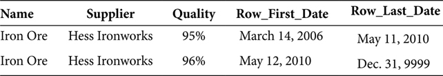
TABLE 13.4
Formula

The Row_Last_Date value for the first row was updated by the Load function. The output of the Transform function identified the row that discontinued as of May 11, 2010, and the row that began as of May 12, 2010. The best practice is to transform these dates in one unit of work to avoid creating any gaps in the time variant metadata.
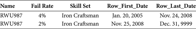
The other attribute that changed in Table 13.1 was the Fail Rate of the RWU987 formula. Table 13.4 shows how the initial row of dimension data for the RWU987 formula might have looked. Formula RWU987 came into effect on Jan. 20, 2005, and has yet to discontinue.
Table 13.5 shows the dimension table updates that occur when extracting Formula data; as of Nov. 25, 2008, the Fail Rate for formula RWU987 was observed to be 2%, which is different from the previous value of 4%.
The Transform function identifies the entity that changed, the row of Formula dimension data that has discontinued as of Nov. 24, 2008, and the row of Formula dimension data that has become effective as of Nov. 25, 2008. The Load function applies the update to the Row_Last_Date of the first row, and inserts the new row, in the Formula dimension table.
Back to the Original Problem
Yes, this explanation of CDC and the application of time variant metadata look very similar to the data displayed in Figure 10.1 and Figure 10.2. That similarity is no accident. The data in Table 13.3 and Table 13.5 is built on the same programming logic that would have built the data in Figure 10.1 and Figure 10.2. So, yes, we have come full circle back to the original problem.
TABLE 13.5
Formula Changed
If you already have an ETL application that feeds dimensional data to a data warehouse, then you probably already have an ETL application, including the CDC function, that uses programming logic very similar to the discussion thus far in this chapter. The logic explained thus far is the basic fundamental logic of all ETL applications, CDC functions, and Load functions.
The ETL portion of this Time Variant Solution Design does not remove any logic or functionality already included in the ETL application, the CDC function, or the Load function. All the functions, features, and homegrown gems already included in the ETL application can remain. So, if you already have an ETL application, then you still have an ETL application—in fact, the same ETL application. And, if you are planning your first ETL application, nothing is lost as all that you intended to include in the ETL application can still be included.
Instance Keys in Dimension ETL
This Time Variant Solution Design requires the addition of Instance Keys to all dimension tables. The following sections will explain the logic by which Instance Keys are generated and incorporated into the data that is then loaded into a dimension table. The examples below provide a mix of Simple Instance Keys and Compound Instance Keys. That mixture of Simple and Compound Instance Keys is for discussion purposes only. In practice, such a mixture of Simple and Compound Instance Keys can be very confusing. For that reason, if possible, a data warehouse should be designed using only Simple Instance Keys or only Compound Instance Keys. If that unilateral design is not an option, then a naming standard should be adopted to identify the time variant key of each table. Because every dimension table will retain its Entity Key and Instance Key, a table with a Simple Instance Key will look very similar to a table with a Compound Instance Key. You don’t want to force the data warehouse users to profile the data in every dimension table to determine its key structure before using each table. For that reason, the best approach is to unilaterally use one Instance Key design (either Simple or Compound) or a naming standard that distinguishes the two from each other.
New Row
A new row of dimension data occurs when an entity, which did not exist before, has been discovered to exist now. The CDC function compared the set of Entity Keys extracted from the operational source system to the set of Entity Keys already in the data warehouse and found a new Entity Key. Table 13.6 and Table 13.7 both show this scenario. If the dimension table is designed to use Simple Instance Keys, then the Transform function, in addition to all the other work it performs, finds the maximum Instance Key value in the dimension table and then increments by one the Instance Key value (e.g., max(Instance Key) + 1) for every Insert row. The row of dimension data in Table 13.6 could be the first row of dimension data for the entity Iron Ore. The Instance Key value 385 would indicate that the Raw Material table previously had 384 rows and that the new Iron Ore row is the 385th row.
TABLE 13.6
Raw Material with a Simple Instance Key

TABLE 13.7
Formula with a Compound Instance Key
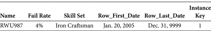
If the dimension table is designed to use Compound Instance Keys, then the Transform function, in addition to all the other work it performs, finds the maximum Instance Key value for that Entity Key in the dimension table and then increments by one the Instance Key value (e.g., max(Instance Key) + 1) for the Insert row for that Entity Key. Finding no previously existing row of dimension data for that Entity Key, the Transform function will assign the value one (e.g., 1). The row of dimension data in Table 13.7 could be the first row of dimension data for the entity RWU987. The Instance Key value 1 would indicate that the Formula table previously had no rows for the RWU987 entity and that the new row is the first row for RWU987.
Updated Row
An updated row of dimension data occurs when an entity, which did exist before and does exist now, has been discovered to have a different attribute value. The CDC function compared the set of Entity Keys extracted from the operational system to the set of Entity Keys already in the data warehouse and found an Entity Key that exists in both sets. The row of dimension data extracted from the operational source system is, however, different from the row of dimension data in the data warehouse in that the two rows have a different attribute value. This means that within the operational source system that attribute value has changed since the previous ETL Cycle.
The Transform function will write a record that will cause the Load function to update the Row_Last_Date of the existing row. That will have the effect of discontinuing the existing row of dimension data. The Transform function will also write a record that will cause the Load function to insert a new row of data for the Iron Ore entity. Table 13.8 shows the final result for the Iron Ore entity.
TABLE 13.8
Raw Material Changed with Simple Instance Keys

The update to the Row_Last_Date of the row previously in effect performed no operation on the Instance Key. The Transform function may include the Instance Key of the row in which the Row_Last_Date will be updated. The Instance Key would allow the Load function to find the updated row more efficiently. Because the Raw Material table uses Simple Instance Keys, the Transform function performs the same algorithm to find the maximum Instance Key value for the table and then increments by one the Instance Key value (e.g., max(Instance Key) + 1) for every Insert row. Every dimension update is composed of a record that discontinues the previously effective row and another record that creates a new Insert row.
The function of defining a new Insert record exists in the Transform output for both New and Updated rows. For that reason, the Instance Key incrementer (e.g., max(Instance Key) + 1) should take as its input data the Insert records from the New and Updated rows. This will allow the Transform function to find the maximum Instance Key and increment the Instance Key in only one iteration rather than two.
An updated row of dimension data with Compound Instance Keys is very similar to an updated row of dimension data with Simple Instance Keys. The CDC function compared the set of Entity Keys extracted from the operational system to the set of Entity Keys already in the data warehouse and found an Entity Key that exists in both sets. The row of dimension data extracted from the operational source system is, however, different from the row of dimension data in the data warehouse in that the two rows have a different attribute value. This means that within the operational source system that attribute value has changed since the previous ETL Cycle.
The Transform function will write a record that will cause the Load function to update the Row_Last_Date of the existing row. That will have the effect of discontinuing the existing row of dimension data. The Transform function will also write a record that will cause the Load function to insert a new row of data for the RWU987 entity. Table 13.9 shows the final result for the RWU987 entity.
TABLE 13.9
Formula Changed with Compound Instance Keys
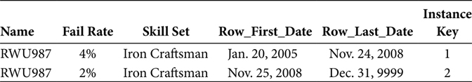
If the dimension table is designed to use Compound Instance Keys, then the Transform function, in addition to all the other work it performs, finds the maximum Instance Key value for that Entity Key in the dimension table and then increments by one the Instance Key value (e.g., max(Instance Key) + 1) for the Insert row for that Entity Key. The row of dimension data in Table 13.9 could be the initial and second row of dimension data for the entity RWU987. In the second row, the Instance Key value 2 would indicate that the Formula table previously had one row for the RWU987 entity and that the new row is the second row for RWU987.
Discontinued Row
The major difference between the standard CDC logic and this Time Variant Solution Design CDC logic is the case of the Discontinued Row. To avoid any gaps in the time frames for an entity, there must be a time frame for the occurrence when an entity ceases to exist. An argument can be made that if an entity ceases to exist, then no enterprise events or transactions will reference it. Any queries that join the nonexistent fact rows to the nonexistent dimension rows will experience no data fallout, as the data doesn’t exist. While this argument may seem true in some level of theory, it does not work well in practice.
The dimension attributes will need a data value that equates to the meaning of “this dimension entity attribute no longer exists.” This is a data model and data design decision. Attributes that are character-based (i.e., alpha characters) can often use the value “n/a.” Attributes that are numeric, with all the arithmetic properties of numeric data, often opt for the null value to avoid any relevance to arithmetic operations. The Row_First_Date and Row_Last_Date will reflect the time frame during which the nonexistent row of dimension data does not exist. If the nonexistence began on Nov. 24, 2010, and continues to persist, then the Row_First_Date would be Nov. 24, 2010, and the Row_Last_Date would be the high-values Dec. 31, 9999, value.
Having established how to present the nonexistence of an Entity Key for a period of time, the CDC function will treat a discontinued entity as an updated entity. For the row previously in effect, a record will be written that will cause the Load function to update the Row_Last_Date of that effective row, rendering it discontinued. For the nonexistence of the entity, an Insert record will be written wherein the attributes are all the “this dimension entity attribute no longer exists” value, the Row_First_Date is the first date on which the Entity Key ceased to exist, and the Row_Last_Date is the high-values Dec. 31, 9999, value.
The Load function will treat the Update row as an update to a previously existing row. The Load function will treat the Insert row as a new row to be inserted. The net effect will be a row for the next time frame that indicates that the entity attributes no longer exist. Even that row, the row that shows the nonexistence of the Entity Key, will have its own Instance Key.
Cascading Instance Keys
Chapter 11 explained the concept of Cascading Instance Keys. Dimension tables relate to other dimension tables via a foreign key/primary key relation. A foreign key that is embedded in a first dimension table will directly join to the primary key of a second dimension table. Figure 11.4 and Figure 11.5 display this design.
Typically the dimension tables that do not have a foreign key to another dimension table are those dimension tables that are at the top of their hierarchies and those dimension tables that are lookup tables. Lookup tables provide a textual description of a cryptic code or indicator value. The vast majority of dimension tables in a data warehouse will reference another dimension table. The Entity Key and Instance Key of a lookup table, which is referenced by a dimension table, will be embedded in the dimension table. The Entity Key and Instance Key of a hierarchical dimension table, which is referenced by a lower hierarchical dimension table, will be embedded in the lower hierarchical table. This is true for both Type 1 and Type 2 time variant dimension tables.
For the purposes of dimension CDC this foreign key/primary key aspect of this Time Variant Solution Design is very important. Cascading Instance Keys dictate the sequence of the ETL jobs for dimension tables. A dimension table can reference the Instance Key of a second dimension table only after the Instance Key for the second dimension table has been generated. That means the ETL jobs cannot be run at random. Instead, the ETL job for a dimension table can only run after the ETL jobs for all tables referenced by that first table have run, including the generation of Instance Keys. For example, if Table A references Table B, and Table B references Table C, then the sequence of ETL jobs would populate Table C, then Table B, and finally Table A. In the case of a lookup table, the ETL job for a lookup table must complete before the ETL jobs for dimension tables that reference that lookup table can run.
That is why Cascading Instance Keys dictate the sequence of ETL jobs. An ETL job flow will typically begin with lookup tables and top-level hierarchy tables. Then, the ETL jobs for the next lower hierarchy level can run, and then the next lower level, and so on, until all the dimension ETL jobs have run. The dimension ETL jobs must complete before a fact ETL job can reference the Instance Keys of the dimension tables.
Dimension Load
The Load function in an ETL application, every ETL application, should contain the least application logic possible. A Load function is like a hinge in a piece of furniture. It is exercised often while also being simultaneously the weakest and most vulnerable link in the piece. For that reason a Load function is optimized by minimizing the application logic, which reduces the number of moving and integrated elements. For that reason, the general rule of Load jobs is that simpler is better. For that reason a Dimension Load should perform only three functions—Delete, Update, and Insert.
Delete
The Delete function is used when a Type 1 dimension row has changed. Because a Type 1 dimension table does not retain history, it also does not retain history rows. For that reason, when an entity is updated, the Load function will delete the previously existing row from a Type 1 dimension table.
The key by which the Delete function can occur is the Entity Key. In a Type 1 dimension table, the Entity Key is the primary key of the table. So, the optimal path by which to delete a row from a Type 1 dimension table is to delete any row from the Type 1 dimension table where the Entity Key of the Type 1 dimension table equals the Entity Key of the Update record written by the CDC function.
Update
The Update function is used when a Type 2 dimension row has changed. The Update function specifically applies a new value to the Row_Last_Date. For a given ETL Cycle the discontinuation of a row is achieved by updating the Row_Last_Date to the date immediately prior to the date for which the ETL Cycle is running. The ETL Cycle may be running for yesterday, two days ago, or any number of days ago. Sometimes an operational source system may delay the availability of data to the Extract function. Such a delay will cause a lag between the date of the ETL Cycle and the date on which the ETL Cycle actually runs. Regardless, the Update function updates the Row_Last_Date to the value of the ETL Cycle date minus one time period, that is, minus one day.
The key by which the Update function can occur is the Instance Key. In a Type 2 dimension table, the Instance Key is the primary key of the table. So, the optimal path by which to update a row from a Type 2 dimension table is to update any row from the Type 2 dimension table where the Instance Key of the Type 2 dimension table equals the Instance Key of the Update record written by the CDC function.
The update function for Type 1 dimension tables and the Update function for Type 2 dimension tables can use the same Update record written by a CDC function. Sharing the Update record with the Delete and Update functions is preferred as it limits the possibility that the Delete and Update functions might use different data. Using the same Update record increases the possibility that corresponding Type 1 and Type 2 dimension tables will stay in synch with each other.
Insert
The Insert function is used in both Type 1 and Type 2 dimension tables. In a Type 1 dimension table an updated entity consists of a Delete function, which removes any previously existing row, and an Insert function, which incorporates the updated dimension row into the Type 1 dimension table. In a Type 2 dimension table an updated entity consists of an Update function, which discontinues the previously existing rows by changing its Row_Last_Date, and an Insert function, which incorporates the updated dimension row into the Type 2 dimension table. Regardless, whether in a Type 1 or Type 2 dimension table, the Insert function does one thing: it inserts. No more, no less, simple and elegant—an Insert function only inserts rows from an Insert record written by the CDC function.
Data Quality
This Time Variant solution has a small margin for error. If your data warehouse has not incorporated an active data quality program into the ETL application, the moment when Type 1 and Type 2 time variant dimension tables are created is the perfect time to incorporate an active data quality program. Data quality is best assessed at all the junctures in an ETL application. The junctures listed thus far, and their potential data quality assessments, are the following:
Extract—After the Extract function retrieves rows from the source system, use an alternate data retrieval method to profile the data that should have been extracted. Compare the data profile to a comparable profile of the Extract file.
Transform—After the Transform function writes the Update/Delete and Insert files:
Verify that the Entity Keys in the Update/Delete file, but not in the Insert file, are in the data warehouse but not in the Extract file.
Verify that the Entity Keys in the Insert file, but not in the Update/Delete file, are in the Extract file but not in the data warehouse.
Verify that the Instance Key of an Entity Key in the Insert file is greater than the maximum Instance Key for the same Entity Key in the data warehouse.
Load—After the Load function has updated the data warehouse from the Update/Delete and Insert files:
Verify that for every Entity Key, exactly one Instance Key applies to each time frame, so that no time frame exists without an Instance Key, which will cause confusion as to which Type 2 time variant dimension row applies to a moment in the past. If the answer is zero Type 2 time variant dimension rows, that’s the wrong answer.
Verify that for every Entity Key, only one Instance Key applies to each time frame, so that no Instance Keys overlap, which will cause confusion as to which Type 2 time variant dimension row applies to a moment in the past. If the answer is two Type 2 time variant dimension rows, that’s the wrong answer.
Verify that for every Entity Key, the row in the Type 1 dimension table is identical to the most recent row in the Type 2 dimension table.
Data quality is a seldom understood, and less frequently implemented, function of an ETL application. The data quality assessments listed above are among the most basic and rudimentary.
Additional data quality assessments are available in Chapter 8 of Building and Maintaining a Data Warehouse. If a time variant data warehouse experiences data quality issues, the potential for data corruption is immense. The best defense against data quality issues is a good offense. The data quality assessments listed above can be the beginnings of a good data quality offense.
Metadata
The simplest form of metadata for a Dimension ETL application is a log table. Each ETL Cycle for each Extract function is assigned a batch number, which is the primary key of the log table. As the extracted data flows through the Transform and Load functions, updates are applied to a series of columns in the log file. Those columns could include such metrics as the following:
Timestamp of the beginning of the Extract function
Number of rows extracted
Timestamp of the ending of the Extract function
Timestamp of the beginning of the Transform function
Number of rows received by the Transform function
Number of “Insert” rows delivered by the CDC function
Number of “Update/Delete” rows delivered by the CDC function
Timestamp of the ending of the Transform function
Timestamp of the beginning of the Load function
Number of “Insert” rows received by the Load function
Number of “Update/Delete” rows received by the Load function
Number of rows inserted
Number of rows updated
Number of rows deleted
Timestamp of the ending of the Load function
The “log table” method is a simple metadata method. The log table method and other metadata measurements are available in Chapter 9 of Building and Maintaining a Data Warehouse. A time variant data warehouse has many moving parts. The time variant aspect renders questions about the data in the data warehouse more difficult to answer. A metadata function will eventually be required when questions arise about how a row, or set of rows, arrived into a dimension table. Chapter 9 of Building and Maintaining a Data Warehouse provides a more comprehensive explanation of the metadata measurements that can render a Type 2 time variant data warehouse easier to understand.
Fact ETL
A Fact table presents the occurrence of an enterprise performing its business functions. Retail sales transactions are extracted from the Retail system, transformed, and then loaded into a Sales table. Manufacturing checkpoints are extracted from the Manufacturing system, transformed, and then loaded into a Manufacturing table. The addition of this Time Variant Solution Design to the Dimension ETL application added the logic to create new Instance Keys. Likewise, the addition of this Time Variant Solution Design to the Fact ETL will only add logic to find existing Instance Keys.
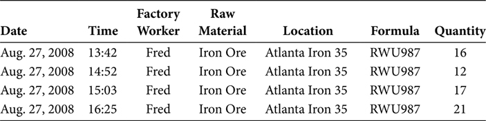
An Extract function retrieves data from the occurrences of a business function. The Transform function identifies the entities involved in that business function. Using the sample data in Table 13.10, a manufacture process includes four data elements—Factory Worker, Raw Material, Location, and Formula—and a quantitative measure of the manufactured output called Quantity. That data will become a row of data in a fact table that presents occurrences of a manufacturing process involving iron ore. For that reason, this sample table might be named Manufacture_Metals_Detail. That row of data in the Manufacturing fact table could look like the data in Table 13.10.
Instance Keys in Fact ETL
TABLE 13.10
Manufacture_Metals_Detail
The addition of Instance Keys to a Fact ETL application changes very little about that ETL application. The source system is still the source system. The business process is still the business process. The entities, quantitative measurements, attributes, and general meaning of rows delivered by a Fact ETL application remain unchanged. Therefore, all the concepts, principles, and best practices already built into an ETL application continue to be the concepts, principles, and best practices...with the addition of Instance Keys.
Every entity in a Fact row is presented by an Entity Key. The Manufacture_Metals_Detail presented in Table 13.10 includes four entities. Those entities are Factory Worker, Raw Material, Location, and Formula. The entity Factory Worker has the Entity Key value of “Fred.” The entity Raw Material has the Entity Key value of “Iron Ore.” The entity Location has the Entity Key value of “Atlanta Iron 35.” The entity Formula has the Entity Key value “RWU987.” Admittedly, these Entity Key values would never actually be used in a data warehouse. They are used here simply to contrast the Instance Key values.
A Fact ETL application incorporates Instance Keys by looking them up. For every entity, the Entity Key and date of the transaction or event represented in the Fact table row are used in a lookup of the dimension table for that entity. First, match on the Entity Key to find all rows for that entity. Then, having identified all rows for that entity, use the date of the transaction or event to find the row of dimension data that matches the Entity Key of that entity and has Row_First_Date and Row_Last_Date values that encompass the date of the transaction or event. Having found the one row of dimension data that matches the Entity Key and encompasses the date of the transaction or event, return the Instance Key in that row of dimension data. That Instance Key will uniquely identify the occurrence of that entity in that dimension table that was effective within the enterprise at the time of the transaction or event.
The Fact ETL does not simply use Type 1 dimension tables for this lookup. To do so would assume that all Fact table data presented to the Fact ETL application can only have occurred during the most recent periodicity time frame of the data warehouse. Such an assumption is most probably completely invalid. So, since we cannot assume that all Fact data presented to the Fact ETL application occurred during the most recent periodicity time frame of the data warehouse, instead we look up the occurrences of each dimension table to avoid placing the time variant entities of a row of Fact table data in the wrong time frame.
Data Quality in Fact ETL
This method must be supported by an attention to data quality. Within a single dimension, for each individual Entity Key, only one Instance Key can apply to each individual time frame. A Dimension ETL post-load data quality assessment should be used to verify that for a single Entity Key, and a single moment in time, exactly one Type 2 time variant dimension row applies to that Entity Key and moment in time. Otherwise, the result set to this lookup operation will cause the Fact ETL application to fail. If the result set has zero rows, the row of Fact data will fail to find a Type 2 Instance Key. If the result set has multiple rows, the Fact ETL will be unequipped to resolve the overlapping dimension rows.
The best-laid plans of ETL analysts and developers often go astray at such junction points between Dimensions and Facts in Fact ETL. You can either programmatically enforce the data quality and integrity of Dimension data in the Dimension ETL or Fact ETL. The alternative is to manually monitor and repair the Fact ETL when it encounters data anomalies. Despite the best efforts to the contrary, data anomalies occur. Data anomalies can be detected and mitigated with the least impact during the Dimension ETL. If they are not mitigated during Dimension ETL, they will reveal themselves during Fact ETL. Data anomalies are most impactful when encountered during Fact ETL.
It is a simple case of “Garbage in...garbage out.” If the Dimension data is certified to be clean before the Fact ETL, the Fact ETL will encounter significantly fewer problems. Chapter 8 of Building and Maintaining a Data Warehouse explained methods for assessing, tracking, and delivering data quality. Data quality does not have to be the vague area south of Mordor. The impact of good and poor data quality is quite tangible and real. The management of data quality can be equally tangible and real. Time variant Fact ETL does not require the use of a data quality program, including data quality assessments, metrics, thresholds, and so on. However, a time variant Fact ETL application will increase in effectiveness, efficiency, and ROI as the quality of its input data increases.
Metadata in Fact ETL
A Fact table may include billions or trillions of rows of data. Business Intelligence (BI) reports wait for that data to arrive. BI applications wait for that data to arrive. Downstream ETL processes wait for that data to arrive. Likewise, a Fact ETL application will need to know its predecessor Dimension ETL applications have completed and the quality of the data delivered by its predecessors. These are the reasons to apply controls to ETL applications, both Dimension ETL and Fact ETL. That level of control is delivered via metadata. Metadata identifies an ETL application job and the data created by that ETL application job. A Metadata application can then inform downstream ETL applications that their predecessors and thresholds have, or have not, been met.
Mistakes happen. When they happen you may need to revise rows of a Fact table. When you need to revise a set of rows of a Fact table you will need a method that will identify that set of Fact rows separately from all other rows of the same Fact table. Again, that level of control is delivered via Metadata. Metadata allows you to identify a specific set of rows of a table that were created by a specific ETL application executed by a specific ETL job. Once the errant rows in a Fact table have been identified, they can be re-created and validated in a separate table. The same dimension lookup function that yielded an incorrect Instance Key previously can be repeated. The corrected and validated rows can be repeated using a corrected Dimension table, yielding corrected results. Once the Fact rows have been re-created and validated in a separate table, they can replace the errant rows in the Fact table.
The textbook definition of Metadata (data about data) is cryptic and uninformative. A better definition of Metadata should include the control, management, and manipulation of data, ETL processes, BI processes, and data quality. These functions, features, and methods are explained in Chapter 9 of Building and Maintaining a Data Warehouse. Time variant ETL does not require Metadata. However, the support of a time variant data warehouse is almost impossible without a Metadata application. So, while Metadata does not inherently create time variance, Metadata enables a data warehouse to control and manage the data and processes in a data warehouse.
Instance Keys—The Manufacturing Example
Before we can incorporate sample data from the Iron Ore manufacturing process first presented in Table 13.10, we need to resolve all the sample Instance Keys to either Simple Instance Keys or Compound Instance Keys. Table 13.11 presents all the Instance Keys as Simple Instance Keys. The Instance Keys in Table 13.11 will be used in the following examples of the Fact table Manufacture_Metals_Detail.
Table 13.12 includes the Fact table rows found in Table 13.10, with the addition of Instance Keys for the entities Factor Worker, Raw Material, Location, and Formula. The Instance Keys, which are Simple Instance Keys in this example, come from Table 13.11.
TABLE 13.11
Manufacturing Dimensions with Simple Instance Keys

The Factory Worker entity Fred has the Instance Key 942 because the dimension row for Fred in the Factory Worker table with the Instance Key value 942 has the Row_First_Date and Row_Last_Date values of April 14, 2007, and Dec. 31, 9999, which inclusively surround the Fact row date of Aug. 27, 2008.
The Raw Material entity Iron Ore has the Instance Key 385 because the dimension row for Iron Ore in the Raw Material table with the Instance Key value 385 has the Row_First_Date and Row_Last_Date values of March 14, 2006, and May 11, 2010, which inclusively surround the Fact row date of Aug. 27, 2008.
The Location entity Atlanta Iron 35 has the Instance Key 234 because the dimension row for Atlanta Iron 35 in the Location table with the Instance Key value 234 has the Row_First_Date and Row_Last_Date values of Feb. 6, 1998, and Dec. 31, 9999, which inclusively surround the Fact row date of Aug. 27, 2008.
The Formula entity RWU987 has the Instance Key 294 because the dimension row for RWU987 in the Formula table with the Instance Key value 294 has the Row_First_Date and Row_Last_Date values of Jan. 20, 2005, and Nov. 24, 2008, which inclusively surround the Fact row date of Aug. 27, 2008.
A Fact ETL application will perform all the lookup operations described in this chapter to find the Instance Keys shown in Table 13.12. If the quality of the Dimension data has been assessed and certified, the Fact ETL lookup processes can be that simple. The lookup processes repeat for every row of data processed by a Fact ETL application.
Most ETL tools include an optimized lookup operation. Often the dimension values are stored in memory so that the lookup operation experiences I/O only on the first “read” operation against a disk drive. Every “read” operation in the lookup that occurs thereafter is a “read” from memory and not from disk. A hand-coded ETL application can achieve the same result by reading all the dimension values into an internal memory array. Then, perform all the lookup operations against the internal memory array rather than against a dimension table stored on disk.
To see time vary, we must vary time. Table 13.13 presents another set of Manufacture_Metals_Detail rows. The set of rows in Table 13.13 occurred on Jan. 20, 2011. The Instance Keys, again in this example, come from Table 13.11.
TABLE 13.12
Manufacture_Metals_Detail Aug 2008

TABLE 13.13
Manufacture_Metals_Detail Jan 2011

The Factory Worker entity Fred has the Instance Key 942 because the dimension row for Fred in the Factory Worker table with the Instance Key value 942 has the Row_First_Date and Row_Last_Date values of April 14, 2007, and Dec. 31, 9999, which inclusively surround the Fact row date of Jan. 20, 2011.
The Raw Material entity Iron Ore has the Instance Key 482 because the dimension row for Iron Ore in the Raw Material table with the Instance Key value 482 has the Row_First_Date and Row_Last_Date values of May 12, 2010, and Dec. 31, 9999, which inclusively surround the Fact row date of Jan. 20, 2011.
The Location entity Atlanta Iron 35 has the Instance Key 234 because the dimension row for Atlanta Iron 35 in the Location table with the Instance Key value 234 has the Row_First_Date and Row_Last_Date values of Feb. 6, 1998, and Dec. 31, 9999, which inclusively surround the Fact row date of Jan. 20, 2011.
The Formula entity RWU987 has the Instance Key 294 because the dimension row for RWU987 in the Formula table with the Instance Key value 294 has the Row_First_Date and Row_Last_Date values of Nov. 25, 2008, and Dec. 31, 9999, which inclusively surround the Fact row date of Jan. 20, 2011.
From the Fact rows in Table 13.12 to the Fact rows in Table 13.13, the Instance Key for Raw Material changed from 385 to 482, and the Instance Key for Formula changed from 294 to 762. They would not, however, exist in two separate Fact tables. Instead, they would exist side by side in a single Fact table, which is shown in Table 13.14.
Type 1 Time Variance
Type 1 Time Variance views all the history of the enterprise as it is now. Chapter 12 provided a solution for organizing the Type 1 dimension tables and views so that they join well with a Fact table that supports both Type 1 and Type 2 time variant dimensions.
A Type 1 query of all the Manufacture_Metals_Detail rows that include the Factory Worker entity named “Fred” will return all the rows in Table 13.14.
TABLE 13.14
Manufacture_Metals_Detail Combined

A Type 1 query of all the Manufacture_Metals_Detail rows that include the Raw Material entity named “Iron Ore” will return all the rows in Table 13.14.
A Type 1 query of all the Manufacture_Metals_Detail rows that include the Location entity named “Atlanta Iron 35” will return all the rows in Table 13.14.
A Type 1 query of all the Manufacture_Metals_Detail rows that include the Formula entity named “RWU987” will return all the rows in Table 13.14.
Type 1 time variant queries make no mention of Instance Keys. Instance Keys provide a join strategy for time variant data. For that reason, Type 1 time variant queries do not need to include Instance Keys.
Type 2 Time Variance
Type 2 time variant queries, however, use only Instance Keys (unless, of course, the Instance Key is a Compound Instance Key that includes the Entity Key). This example uses Simple Instance Keys. So, in this example Type 2 time variant queries use only Instance Keys, and never use Entity Keys.
A Type 2 query of all the Manufacture_Metals_Detail rows that include the Factory Worker Instance Key 942 will return all the rows in Table 13.14.
A Type 2 query of all the Manufacture_Metals_Detail rows that include the Raw Material “Iron Ore” with a Quality rating of 95%, which is in the Raw Material row with Instance Key 385, will return the rows in Table 13.14 dated Aug. 27, 2008.
A Type 2 query of all the Manufacture_Metals_Detail rows that include the Raw Material “Iron Ore” with a Quality rating of 96%, which is in the Raw Material row with Instance Key 482, will return the rows in Table 13.14 dated Jan. 20, 2011.
A Type 2 query of all the Manufacture_Metals_Detail rows that include the Location Instance Key 234 will return the rows in Table 13.14.
A Type 2 query of all the Manufacture_Metals_Detail rows that include the Formula “RWU987” with a Fail Rate of 4%, which is in the Formula row with Instance Key 294, will return the rows in Table 13.14 dated Aug. 27, 2008.
A Type 2 query of all the Manufacture_Metals_Detail rows that include the Formula “RWU987” with a Fail Rate of 2%, which is in the Formula row with Instance Key 762, will return the rows in Table 13.14 dated Jan. 20, 2011.
The Dimension and Fact tables have no direct connection between a Quality rating of 95% and Aug. 27, 2008, between a Quality rating of 96% and Jan. 20, 2011, between a Fail Rate of 4% and Aug. 27, 2008, or between a Fail Rate of 2% and Jan. 20, 2011. The connection between these dimension attributes and dates in a Fact table is the Instance Keys that are embedded in a row of Fact data by the Fact ETL. Those Instance Keys in a row of Fact data join directly to one, and only one, row of Dimension data. Each row of Dimension data is uniquely identified by an Instance Key because the Dimension ETL application that populated that Dimension table assigned that Instance Key to one, and only one, row of that Dimension table.
Obviously, therefore, all the Dimension ETL must be complete (meaning the Dimension tables have been populated with data) before the Fact ETL can begin. Otherwise, the Instance Key lookup operation will not have a current set of Instance Keys to look up.
Summary ETL
After a Fact ETL application has completed the updates to a Fact table, a Summary application can summarize data from that Fact table. Summaries in a data warehouse are created for performance reasons. If data warehouse users consistently query a Fact table, summing by one of its dimensions, a Summary process can remove that resource consumption from the data warehouse by performing that sum operation once and then storing the result set in a separate table. Thereafter, data warehouse customers need only query the separate summary table. That reduces the occurrence of the sum operation from near ad infinitum throughout the day to once during off-peak hours.
The phrase “summing by one of its dimensions” is a reference to both the structure of a Fact table and the structure of the SQL in a query. In its simplest form, a summing query will include a SUM clause and a GROUP BY clause, as shown in Figure 13.1.
The possible dimensions in Table 13.14, which could be included in a Sum operation, are Factory Worker, Raw Material, Location, and Formula. The only quantitative value in Table 13.14 is the column named Quantity. The Fact table in Table 13.14 presents both Entity Keys and Instance Keys. So, it is possible that a summation operation can leverage either the Entity Keys or the Instance Keys.

FIGURE 13.1
SUM SQL.
Type 1 Summary ETL
Entity Keys are associated with Type 1 Time Variance. A Summary ETL application is a Type 1 Summary ETL application when it references Entity Keys, rather than Instance Keys. Figure 13.2 shows a summation query that references only Entity Keys. The result set will include only Entity Keys and will therefore be a Type 1 result set.
Type 2 Summary ETL
Instance Keys are associated with Type 2 Time Variance. A Summary ETL application is a Type 2 Summary ETL application when it references Instance Keys, rather than Entity Keys. Figure 13.3 shows a summation query that references only Instance Keys. The result set will include only Instance Keys and will therefore be a Type 2 result set.
From the perspective of a Summary ETL application, a Type 2 Summary table and a hybrid Type 1/Type 2 Summary table are extremely similar. A hybrid Type 1/Type 2 Summary table contains both the Entity Key and the Instance Key for each dimension. Therefore, the SQL in the Summary ETL for a hybrid Type 1/Type 2 Summary table, shown in Figure 13.4, includes both the Entity Key and the Instance Key for every dimension. Because the Instance Key is the lower granularity of the two keys, the Instance Key, rather than the Entity Key, determines the cardinality of the summation operation and the output result set.

FIGURE 13.2
Type 1 Time Variant SUM SQL.
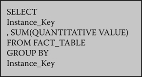
FIGURE 13.3
Type 2 Time Variant SUM SQL.
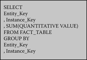
FIGURE 13.4
Hybrid Type 1/Type 2 Time Variant SUM SQL.
Metadata, Data Quality, and the Like
All the Metadata processes included in Dimension and Fact ETL are also included in Summary ETL. Summary ETL processes require the same level of management, control, and quality assessment as other ETL processes. Rather than repeat the previous descriptions of Metadata and Data Quality processes already covered, please refer back to Chapters 8 and 9 of Building and Maintaining a Data Warehouse, as both the Metadata and Data Quality applications are explained there.